remote sensing Article
Transformation Model with Constraints for High-Accuracy of 2D-3D Building Registration in Aerial Imagery Guoqing Zhou 1,2, *, Qingli Luo 2 , Wenhan Xie 3 , Tao Yue 1 , Jingjin Huang 2,4 and Yuzhong Shen 5 1 2 3 4 5
*
Guangxi Key Laboratory for Geospatial Informatics, Guilin University of Technology, Guilin 541004, China;
[email protected] The Center for Remote Sensing, Tianjin University, No. 92, Weijin Road, Nankai District, Tianjin 300072, China;
[email protected] (Q.L.);
[email protected] (J.H.) Chinese Academy of Surveying and Mapping, 28 Lianhuachi West Road, Beijing 100830, China;
[email protected] School of Precision Instrument and Opto-Electronics Engineering, Tianjin University, No. 92, Weijin Road, Nankai District, Tianjin 300072, China Department of Modeling, Simulation, and Visualization Engineering, Old Dominion University, Norfolk, VA 23529, USA;
[email protected] Correspondence:
[email protected]; Tel.: +86-773-589-6073
Academic Editors: Devrim Akca, Soe Myint and Prasad S. Thenkabail Received: 27 January 2016; Accepted: 26 May 2016; Published: 16 June 2016
Abstract: This paper proposes a novel rigorous transformation model for 2D-3D registration to address the difficult problem of obtaining a sufficient number of well-distributed ground control points (GCPs) in urban areas with tall buildings. The proposed model applies two types of geometric constraints, co-planarity and perpendicularity, to the conventional photogrammetric collinearity model. Both types of geometric information are directly obtained from geometric building structures, with which the geometric constraints are automatically created and combined into the conventional transformation model. A test field located in downtown Denver, Colorado, is used to evaluate the accuracy and reliability of the proposed method. The comparison analysis of the accuracy achieved by the proposed method and the conventional method is conducted. Experimental results demonstrated that: (1) the theoretical accuracy of the solved registration parameters can reach 0.47 pixels, whereas the other methods reach only 1.23 and 1.09 pixels; (2) the RMS values of 2D-3D registration achieved by the proposed model are only two pixels along the x and y directions, much smaller than the RMS values of the conventional model, which are approximately 10 pixels along the x and y directions. These results demonstrate that the proposed method is able to significantly improve the accuracy of 2D-3D registration with much fewer GCPs in urban areas with tall buildings. Keywords: 2D-3D registration; transformation model; building; aerial image; urban
1. Introduction Texturing three-dimensional (3D) buildings at a large scale for the generation of a photorealistic urban environment has been an important research topic in the computer vision [1–4], computer graphics [5] and remote sensing communities [6]. The prerequisite for texturing 3D buildings is high accuracy in the geometric alignment of 2D texture images, which are captured by different types of devices, such as airborne and spaceborne platforms, with their corresponding 3D models without textures, which are represented by various geometric data structures. This process is called 2D-3D registration. Researchers encountered various unique real-world problems and have developed a variety of approaches for 2D-3D registration. Remote Sens. 2016, 8, 507; doi:10.3390/rs8060507
www.mdpi.com/journal/remotesensing
Remote Sens. 2016, 8, 507 Remote Sens. 2016, 8, 507 registration. Researchers
2 of 17 encountered various unique real-world problems and have developed a variety of approaches for 2D-3D registration. A commonly-adopted transformation model for a given ground point G can be expressed by: A commonly-adopted transformation model for a given ground point G can be expressed by:
˛ ˛G ¨ X S ˛ x¨ X g xg XS XG = Y ‹+ R (ω , φ , κ ) y˚ ‹ ˚ Y‹ ˚ g yg ‚ ˝ ˝ YG ‚G“ ˝ YSS ‚` Rpω, φ, κq ZS z g zg ZG Z G Z S ¨
(1) (1)
where (XG, YG, ZG)T are the coordinates of the point G in 3D space with respect to a geographic where (XG , YG , ZG )T are the coordinates of the point G in 3D space with respect to a geographic coordinate system, (XS, YS, ZS)TTare the center of the perspective projection, which is the translation coordinate system, (XS , YS , ZS ) are the center of the perspective projection, which is the translation vector between the origins of the 2D image coordinate system and the geographic coordinate system, vector between the origins of the 2D image coordinate system and the geographic coordinate system, (xg, yg, zg)TT are the image coordinates of the given ground point G with respect to the image (xg , yg , zg ) are the image coordinates of the given ground point G with respect to the image coordinate coordinate system, φ, ω and k are three rotation angles and R(φ, ω, k) is a 3D orthogonal rotation system, ϕ, ω and k are three rotation angles and R(ϕ, ω, k) is a 3D orthogonal rotation matrix as follows, matrix as follows, ¨ ˛ cosφcosk ´ cosωsinφcosk φ cos k cos ωcosωsink sin k + sin`ωsinωsinφcosk sin φ cos k sinsinωsink ω sin k − cos ω sin φ cos k cos ˚ ‹ (2) ` cosωsinφsink ˝ φ´cosφsink R =R “ sin k cos ωcosωcosk cos k − sin´ωsinωsinφsink sin φ sin k sinsinωcosk ω cos k + cos ω sin φ sin k ‚ − cos (2) sinφ ´sinωcosφ cosωcosφ
sin φ
− sin ω cos φ
cos ω cos φ
T Traditional Traditional 2D-3D 2D-3D registration registration methods methods solve solve for for the the camera’s camera’sposition position(X (XSS,, YYSS,, ZZSS))T and and its its orientation matrix R in Equations (1) and (2). However, none of the distortion models are perfect. orientation matrix R in Equations (1) and (2). However, none of the distortion models are perfect. Any Any distortion distortion model model cannot cannot completely completely describe describe the the distortion distortion over over the the entire entire image image plane, plane, i.e., i.e., the the residual errors (incomplete correction) still remain no matter what kind of distortion model is adopted. residual errors (incomplete correction) still remain no matter what kind of distortion model is As a result, accuracy image coordinates in the entire image plane is asymmetric (see Figure(see 1). adopted. Asthe a result, the of accuracy of image coordinates in the entire image plane is asymmetric This phenomenon has been demonstrated in [7] and it becomes obvious for a big dimension of aerial Figure 1). This phenomenon has been demonstrated in [7] and it becomes obvious for a big images, especially inimages, which aespecially much higher and bigger building imaged on abuilding large area in the image dimension of aerial in which a much higheris and bigger is imaged on a plane [8]. Two constraint conditions are added into the traditional transformation model (Equation (1)) large area in the image plane [8]. Two constraint conditions are added into the traditional to increase the accuracy, reliability(1)) andtorobustness of accuracy, the imagereliability distortionand correction. For of thethe example transformation model (Equation increase the robustness image shown in Figure 1, the image distortion in Region 1 is different from that of Regions 2 and 3. If a distortion correction. For the example shown in Figure 1, the image distortion in Region 1 is different conventional transformation model (e.g., photogrammetry backward intersection (PBI)) is applied from that of Regions 2 and 3. If a conventional transformation model (e.g., photogrammetry to register intersection such a 2D image containstovarious dissymmetric with various a 3D object backward (PBI))that is applied registerand such a 2D imagedistortions that contains and represented by a rigid model, errors in the 2D-3D registration are undoubtedly unavoidable. This dissymmetric distortions with a 3D object represented by a rigid model, errors in the problem is especially for high-rise buildings becauseisthe bottom and top offor a high-rise 2D-3D registration areprofound undoubtedly unavoidable. This problem especially profound high-rise building are affected by different distortions in the same image. To avoid this problem, this paper buildings because the bottom and top of a high-rise building are affected by different distortions in presents a novel algorithm using two types of geometric constraints, i.e., co-planar and perpendicular the same image. To avoid this problem, this paper presents a novel algorithm using two types of conditions, to improvei.e., theco-planar accuracy and of the 2D-3D registration. Thetotwo conditions added in geometric constraints, perpendicular conditions, improve the accuracy of the the proposed transformation model, in relation to the original rigorous transformation model, can 2D-3D registration. The two conditions added in the proposed transformation model, in relation be to summarized in the following. the original rigorous transformation model, can be summarized in the following.
Figure 1. Error of the 2D-3D registration caused by both various and dissymmetric image distortions, Figure 1. Error of the 2D-3D registration caused by both various and dissymmetric image distortions, displacement and a rigid 3D object model. displacement and a rigid 3D object model.
2
Remote Sens. 2016, 8, 507
(1) (2)
3 of 17
Co-planar condition: The photogrammetric center, a line in the object coordinate system and the corresponding line in the image coordinate system are in the same plane. Perpendicular condition: The constraint requires that if two lines are perpendicular in the object coordinate system, their projections are perpendicular in the image coordinate system.
The remainder of this paper is organized as follows: Section 2 briefly overviews related work; Section 3 focuses on the development of a rigorous transformation model; Sections 4 and 5 evaluate the correctness and accuracy of the proposed method and compare it to other existing methods; Section 6 summarizes the major contributions and advantages of the proposed method. 2. Related Work 2D-3D registration for different applications has been a very active research area in the last few decades. Researchers have developed a wide range of 2D-3D registration methods; papers in the existing literature provide an overall survey and study of various registration methods, such as [9–17]. Most of the registration methods consist of four steps as follows: ‚
‚ ‚
‚
Feature detection: Existing methods can be classified into feature-based or intensity-based methods. Feature-based methods use point features, linear features and areal features extracted from both the 3D urban surface/building model and 2D imagery as the common feature pairs and then align the corresponding feature pairs via a transform model. This method has been widely applied in computer vision [18–23] and medical image processing [24,25]. Intensity-based methods utilize the intensity-driven information, such as texture, reflectance, brightness, and shadow, to achieve high-accuracy in 2D-3D registration [11,13,26]. These features, which are called ground control points (GCPs) in remote sensing, can be detected manually or automatically. Feature matching: The relationship between the features detected from the two images is established. Different feature similarity measures are used for the estimation. Transform model estimation: The transform type and its parameters between two images are estimated by certain mapping functions based on the previously-established feature correspondence. Image resampling and transformation: The slave image is resampled and transformed into the frame of the reference image, according to the transformation model and interpolation technique.
Among the previous efforts, imaging geometry has been utilized as a rigorous transformation model by some researchers, such as [26–32] suggested integrating single straight lines into the orientation of images for building reconstruction and/or building recognition. Habib et al. [33] proposed that straight lines be utilized as constraints in photogrammetric bundle adjustment to solve the interior orientation parameters (IOPs) of the camera and the exterior orientation parameters (EOPs) of aerial images. Two major advantages lie in that: (1) straight lines are employed to enhance the reliability of bundle adjustment; and (2) the IOPs are considered as unknown parameters to be solved in the model. The disadvantages of this method lie in that: (1) the straight line constraint is not as strong as that of co-planarity, because this type of constraint does not combine the image space, object space and perspective center; (2) the straight line constraint enhances only the accuracy along a straight line in theory, whereas the accuracy along other directions, such as that perpendicular to the straight line, becomes relatively weak. Zhang et al. [34] developed a methodology to co-register the laser scanning data and aerial images over urban areas. The method considers a linear feature as observed primitives and uses coplanar condition as error equations to solve for the EOP of the digital image. One advantage of this method is that it extends the straight line constraint into the coplanar constraint, which in fact combines features in object space, image space and the perspective center. One disadvantage is that it considers digital cameras as a rigid body for which the IOPs are known and are computed independently. Considering the advantages and disadvantages of the two foregoing methods (i.e., [33,34]), this paper presents two types of constraint conditions, i.e., coplanar and perpendicular conditions. This
Remote Sens. 2016, 8, 507
4 of 17
idea comes from the fact that Zhou et al. [8] demonstrated that two aerial images over an urban area will have different accuracy of registration even with the same digital building model (DBM) and the same algorithm. This implies that highly accurate 2D-3D registration will not be achievable if constraint conditions are not applied. 3. Rigorous Transformation Model We first briefly describe the fundamental concepts of the conventional rigorous transformation model, which is based on imaging geometry. For more detailed information, please refer to existing literature [27–29]. This paper only considers aerial photography. The conventional rigorous transformation model is represented by: r pX ´Xsq`r pY ´Ysq`r pZ ´Zsq
x g ´ x0 “ ´ f r11 pXG ´Xsq`r12 pYG ´Ysq`r13 pZG ´Zsq “ ´ f x 31
32
G
33
G
G
(3)
r pX ´Xsq`r pY ´Ysq`r pZ ´Zsq
y g ´ y0 “ ´ f r21 pXG ´Xsq`r22 pYG ´Ysq`r23 pZG ´Zsq “ ´ f y 31
32
G
33
G
G
where f, x0 , y0 are the camera’s IOP and ri,j (i = 1, 2, 3; j = 1, 2, 3) are components of the rotation matrix R(ω, φ, k), which was described in Equation (2). Considering two types of imagery distortions, radial and decentering, the image coordinates in Equation (3) can be modified by: x1g “ x g ` δx ´ x0 y1g “ y g ` δy ´ y0
(4)
where (x1 g, y1 g) are the distortion-free image coordinates after correction and δx, δy are corrections through the imagery distortion models below: radial hkkkkkkkikkkkkkkj
decentering hkkkkkkkkkkkkkkikkkkkkkkkkkkkkj
δx “ κ1 x g px2g ` y2g q ` ρ1 p3x2g ` y2g q ` 2ρ2 x g y g radial hkkkkkkkikkkkkkkj
(5)
decentering hkkkkkkkkkkkkkkikkkkkkkkkkkkkkj
δy “ κ1 y g px2g ` y2g q ` ρ2 p3x2g ` y2g q ` 2ρ1 x g y g where k1 , ρ1 and ρ2 are the coefficients of radial distortion and decentering, respectively, and xg , yg are the coordinates of a target point in a defined image coordinate system. Because Equation (3) is not linear, it must be linearized with respect to both IOPs and EOPs. The vector form of the registration model can be expressed by: V “ A 1 X1 ` A 2 X2 ´ L
(6)
where X1 represents EOPs; X2 denotes IOPs; V is the residual error matrix; and A1 and A2 are their coefficients, whose partial derivatives with respect to the registration parameters can be found in [35]. The vectors in Equation (6) are X1 = (φ, ω, k, XS , YS , ZS )T , X1 = [k1 , ρ1 , ρ2 ], V “ pVx g , Vy g q, » A1 “ –
B fx B Xs B fy B Xs
˜ L“
B fx BYs B fy BYs
Lxg Ly g
¸
B fx B Zs B fy B Zs
» “–
B fx Bφ B fy Bφ
B fx Bω B fy Bω
B fx Bκ B fy Bκ
fi
»
fl , A2 “ –
B fx B κ1 B fy B κ1
B fx B ρ1 B fy B ρ1
r pX ´Xsq`r pY ´Ysq`r pZ ´Zsq
x1g ´ f r11 pXG ´Xsq`r12 pYG ´Ysq`r13 pZG ´Zsq 31
G
32
G
33
G
r pX ´Xsq`r pY ´Ysq`r pZ ´Zsq
y1g ´ f r21 pXG ´Xsq`r22 pYG ´Ysq`r23 pZG ´Zsq 31
G
32
G
33
B fx B ρ2 B fy B ρ2
fi fl
fi fl
G
The registration parameters in Equation (6) are conventionally solved by least adjustment estimation using a number of well-distributed GCPs. As mentioned previously, the conventional registration model is not robust for high-rise buildings in urban areas. Therefore, this paper proposes two types of conditions, co-planarity and
Remote Sens. 2016, 8, 507 Remote Sens. 2016, 8, 507
5 of 17
As mentioned previously, the conventional registration model is not robust for high-rise buildings in urban Therefore, paper proposes two types conditions, co-planarity and perpendicularity, as areas. constraints to the this conventional model Equation (6).ofMathematically, the two types perpendicularity, as constraints to the conventional model Equation (6). Mathematically, the two of conditions are described as follows. types of conditions are described as follows. 3.1. Coplanar Condition 3.1. Coplanar Condition The straight line condition does not combine the features in image space, object space and The straight condition doesproposes not combine the features in image space, objectis space perspective center;line thus, this paper a coplanar constraint condition, which similarand to perspective center; thus, this paper proposes a coplanar constraint condition, which is similar to (Zhang et al., 2005). As shown in Figure 2, given two points P and Q on the object surface, their (Zhang et al., 2005). shown Figure 2, points, given two points exposure P and Q center), on the P, object their corresponding imageAs points are pinand q. Five O (camera Q, p surface, and q, should corresponding image points are p and q. Five points, O (camera exposure center), P, Q, p and q, theoretically be coplanar. The mathematical model that describes the coplanar condition using three Ñ Ñ Ñ should theoretically be coplanar. The mathematical model that describes the coplanar condition vectors OP, OQ and Op is: → → → using three vectors OP , OQ and Op is: ˇ ˇ ˇ ˇ u v w p p p ˇ ˇ up vp wp ˇ ˇ (7) ˇ XP ´ XS YP ´ YS ZP ´ ZS ˇ “ Fp “ 0 ˇ X P − X S YP − YS Z P − Z S = Fˇ p = 0 (7) ˇ XQ ´ XS YQ ´ YS ZQ ´ ZS ˇ
XQ − XS
YQ − YS
ZQ − Z S
where ZQQ)) are are coordinates coordinates of of the the ground is the the residual residual error error matrix; matrix; (X (XPP,, YYPP,, Z ZPP)) and and (X (XQQ,, Y YQ Q,, Z ground where FFPP is points P, Q with respect to the ground coordinate system, respectively; (u , v , w ) are coordinates of points P, Q with respect to the ground coordinate system, respectively; (uPP, vPP, wPP) are coordinates of the the image image point point pp with with respect respect to to the the camera camera coordinate coordinate system. system.
Figure 2. The geometry for the coplanar condition. Figure 2. The geometry for the coplanar condition.
Combining Equations (1) and (3), Equation (7) yields Combining Equations (1) and (3), Equation (7) yields
up vp w p ˇ ˇu p v p w p ˇ ˇ ˇ ˇ ˇ u ˇ ' p 'vp ' wp ˇ uXp − X vYp − Y w p ˇ ˇ ˇ Z P − Z Sˇ = ˇX P YP Z P = Fˇ p = 0 P S P S ˇ 1 1 1 Y Z ˇ “ Fp “ 0 ˇ XP ´ XS YP ´ YS ZP ´ ZS ˇ “ ˇ X ˇ X − X Y − Y Z Q − Z Sˇ ˇX Q' 1P YQ' P1 Z Q' 1P ˇ ˇ XQ ´QXS SYQ ´QYS S ZQ ´ ˇ ˇ ˇ X Y Z ZS Q Q Q
(8) (8)
where: where: ' '
( X P , YP , ZP' ) = ( X P − X S , YP − YS , ZP − ZS ) , ( XQ' ,YQ' , ZQ' ) = ( XQ − X S ,YQ −YS , ZQ − ZS ) .
1 1 1 1 1 1 pX P , YP , ZP q “ pX P ´ XS , YP ´ YS , ZP ´ ZS q, pXQ , YQ , ZQ q “ pXQ ´ XS , YQ ´ YS , ZQ ´ ZS q. Let: ' Let: A=Y ⋅ Z ' − Y ' ⋅ Z ' , B = Z ' ⋅ X ' − Z ' ⋅ X ' , C = X ' ⋅Y ' − X ' ⋅Y ' ; P
Q
Q
P
P
Q
Q
P
P
Q
Q
P
1 ´ Y 1 ¨ Z1 , B “ Z1 ¨ X 1 ´ Z1 ¨ X 1 , C “ X 1 ¨ Y 1 ´ X 1 ¨ Y 1 ; A “ YP1 ¨ ZQ P Pas: Q P P P Q Q Q Equation (7) canQbe rewritten Equation (7) can be rewritten as:
FP = A ⋅ u p + B ⋅ v p + C ⋅ wp FP “ A ¨ u p ` B ¨ v p ` C ¨ w p
5
(9) (9)
Remote Sens. 2016, 8, 507
6 of 17
With the established coplanar constraint Equation (9), considering differential terms with respect to the unknown parameters when linearizing using Taylor’s series, Equation (9) can also be rewritten using a differential form as, ˇ ˇ u p ` du P ˇ ˇ 1 ˇ XP ` dXP ´ dXS ˇ 1 ˇ XQ ` dXQ ´ dXS
v p ` dv P YP1 ` dYP ´ dYS 1 ` dY ´ dY YQ Q S
w p ` dw P ZP1 ` dZP ´ dZS 1 ` dZ ´ dZ ZQ Q S
ˇ ˇ ˇ ˇ ˇ “ Fp “ 0 ˇ ˇ
(10)
BF
where dp.q “ Bp.pq , and Equation (10) is rewritten as: A1P ¨ dφ ` A2P ¨ dω ` A3P ¨ dκ ` A4P ¨ dXS ` A5P ¨ dYS ` A6P ¨ dZS ` FP “ 0
(11)
where: p
A1 “ A ¨ r´r31 x1P ´ r32 y1P ` r33 f s ` C ¨ rr11 x1p ` r12 y1p ´ r13 f s p
A2 “ A ¨ rp´sinφcosωsinκqx1p ` p´sinφcosωcosκqy1p ´ f sinφsinωs` B ¨ rp´sinφsinκqx1p ` p´sinωcosκqy1p ` f cosωs` C ¨ rpcosφcosωsinκqx1p ` pcosφcosωcosκqy1p ` f cosφsinωs p
A3 “ A ¨ rr12 x1p ´ r11 y1p s ` B ¨ rpcosωcosκqx1p ` p´cosωsinκqy1p s ` C ¨ rr32 x1p ´ r31 y1p s p
p
1 ´ Y 1 qw ` pZ1 ´ Z1 qv s, A “ ´rpX 1 ´ X 1 qw ` pZ1 ´ Z1 qu s A4 “ ´rpYQ p p P P p P P p Q Q Q 5 p
1 ´ X 1 qv ` pY 1 ´ Y 1 qu s, px1 , y1 q A6 “ ´rpXQ p p P p P p Q
are image coordinates of point p on the image plane after all corrections in Section 3.1; other symbols are the same as above. Equation (11) is rewritten in vector form as below: C1 X1 ` W1 “ 0
(12)
where: C1 “ r A1P X1 “ r dω W1 “ FP .
A2P A3P A4P A5P A6P s, dϕ dk dXS dYS dZs s,
3.2. Perpendicular Condition The perpendicularity constraint in 3D space is added to ensure preservation of the registered 2D and 3D pairs after applying registration transformation. As shown in Figure 3, suppose that AB and BC are two edges of a flat house roof, and their corresponding edges in the 2D image plane are ab and bc. Suppose that the coordinates of A, B and C are (XA , YA , ZA ), (XB , YB , ZB ) and (XC , YC , ZC ), respectively, in the object coordinate system. For a flat-roof, cube house, the heights (i.e., Z coordinates) of A, B and C are the same, and the line segments AB and BC are perpendicular to each other. If AB is not perpendicular to BC and the angle between them is θ, i.e., B deviates from its correct position at B1 , a line from C to O is drawn, and CO is perpendicular to AB1 . l is the distance between B and O and can be expressed by [8]: l “ pXC ´ XB qcosθ ` pYC ´ YB qsinθ “ pYC ´ YB qpYB ´ YA q{S AB ` pXC ´ XB qpXB ´ X A q{S AB
(13)
where SAB is the length of the segment AB. Theoretically, the distance l should be zero. Thus, the differential form of Equation (13) is: l0 ` ∆l “
rpYC ´ YB qpYB ´ YA q{S AB ` pXC ´ XB qpXB ´ X A q{S AB s` rpXB ´ X A q∆XC ` pYB ´ YA q∆YC ` pXB ´ XC q∆X A ` pYB ´ YC q∆YA ` pXC ´ 2XB ` X A q∆XB ` pYC ´ 2YB ` YA q∆YB s{S AB “ 0.
(14)
Remote Sens. 2016, 8, 507
l0 + Δl = [(YC − YB )(YB − YA ) / S AB + ( X C − X B )( X B − X A ) / S AB ] + Remote Sens. 2016, 8, 507 [( X B − X A )ΔX C + (YB − YA )ΔYC + ( X B − X C )ΔX A + (YB − YC )ΔYA + ( X C − 2 X B + X A )ΔX B + (YC − 2YB + YA )ΔYB ] / S AB = 0. Equation (14) can be rewritten in matrix form as below: Equation (14) can be rewritten in matrix form as below: fi fiT » » T ´BX−C X C X AA Δ∆X XB X ffi — ∆Y ffi — Y ´Y B Y − CY ffi — ΔYAA ffi — B C ffi — — X ´ 2X ffi — C B ` X A ffi — ∆X B ffi — X C − 2 X B + XffiA — ΔX B ffi ` rpXC ´ XB qpXB ´ X A q ` pYC ´ YB qpYB ´ YA qs “ 0 — YC ´ 2YB ` YA ffi — ∆YB ffi + [( X C − X B )( X B − X A ) + (YC − YB )(YB − YA )] = 0 — Y ffi — 2YAB + YAffi −X fl – Δ – XYBC ´ ∆XBC fl
YB X ´ BY− A XA YB − YA
7(14) of 17
(15) (15)
Δ∆Y X CC ΔYC
Equation (15) can be then rewritten in vector form as:
Equation (15) can be then rewritten in vector form as: C2 Xˆ 2 ` W2 “ 0
C2 Xˆ 2 +W2 = 0
where: where: ” B ´ XC q pYB ´ YC q pXC ´ 2X B ` X A q pYC ´ 2YB ` YA q pX B ´ X A q C2 =C[(2X“B −”XpX C ) (YB −YC ) (XC −2XB + XA) (YC −2YB +YAı) (XB − XA) (YB −YA)] , T ˆ 2 “ ∆X A ∆YA ∆XB ∆Y , ∆XC ∆YC T B ˆX =X[Δ XA ΔYA ΔXB ΔYB ΔXC ΔYC ] , 2 W2 “ pXC ´ XB qpXB ´ X A q ` pYC ´ YB qpYB ´ YA q. W 2 = ( X C − X B )( X B − X A ) + (YC − Y B )( Y B − Y A ) .
(16) (16) ı pYB ´ YA q
,
Figure 3. The geometry of the perpendicular condition. Figure 3. The geometry of the perpendicular condition.
3.3. Solution of Registration Parameters 3.3. Solution of Registration Parameters By combining Equations (6), (12) and (16), we have: By combining Equations (6), (12) and (16), we have: $ V = A1 X 1 + A2 X 2 − L ’ 2´L & V “CA1XˆX1+`WA2=X0 C Xˆ ` 1 1 1 W “ 0 1 1 1 ’ % Xˆ 2 2+“ W02 = 0 C2 XˆC 2 2` W
7
(17) (17)
Remote Sens. 2016, 8, 507
8 of 17
Furthermore, Equation (17) can be rewritten as: #
where: ´ Cx “ C1
C2
¯T
´ , Wx “
W1
W2
¯T
V “ DδX ´ L Cx δX ` Wx “ 0
´ , D“
(18)
¯ A1
A2
,
δX “ p∆φ ∆ω ∆κ ∆XS ∆YS ∆ZS ∆X A ∆YA ∆Z A ¨ ¨ ¨ ∆X N ∆YN ∆ZN qT Equation (18) is the model derived in this paper for 2D-3D registration. Distinct from the existent conventional model used for 2D-3D registration in Equation (7), this model is called the rigorous model in this paper. As can be seen in Equation (18), this registration model combines the linear edges and conventional point features of a building. This model should therefore achieve higher accuracy and reliability than the conventional model. Equation (18) is usually solved using least-squares estimation, which is expressed as [36]: Φ “ V T V ` 2KST pCX δX ` WX q “ min (19) With least-squares estimation, the solution normal equation matrix can be written as: #
T D δX ` C T K ` D L “ 0 DX X X X S CX δX ` 0KS ` WX “ 0
(20)
where Ks is an introduced unknown matrix (for its details, please refer to [37]). If the number of total ` ˘T observation equations is M, the dimension of Ks is M ˆ 1, i.e., KS “ KS1 , KS2 , ¨ ¨ ¨ , KS M . Let NXX “ DxT Dx ; Equation (20) can be rewritten as: ˜
NXX CX
T CX 0
¸˜
¸ δX KS
˜ `
TL DX WX
¸ “0
(21)
The solution of unknown parameters would be: #
δX “ ´pQ12 D T L ` Q12 WX q KS “ ´pQ21 D T L ` Q22 WX q
(22)
where Qij (i, j = 1, 2) is the components of the covariance matrix, which is an inverse of the normal matrix, i.e., ˜ ¸´1 ˜ ¸ T NXX CX Q11 Q12 “ (23) T CX 0 Q21 Q22 3.4. Accuracy Evaluation The standard deviations of the unit weight and unknown parameters are typically used to evaluate the quality of adjustment and the accuracy of adjusted unknown parameters. The standard deviation of the unit weight δ0 is computed by: c VTV (24) δ0 “ r where V is the residual vector and r is the redundancy of the observation equation.
Remote Sens. 2016, 8, 507
3.5. Discussion
Remote Sens. 2016, 8, 507
9 of 17
3.5.1. Coplanar and Collinear Constraint 3.5. Discussion Lines have been used as registration primitives in previous work. As shown in Figure 4, if any three points B′, E′, C′ in object space are collinear, the collinear constraint condition can be 3.5.1. Coplanar and Collinear Constraint established according to the method proposed by [8,33]. We can analyze the constraint condition of lines.Lines have been used as registration primitives in previous work. As shown in Figure 4, if any three points B1 , E1 , C1 in object space are collinear, the collinear constraint condition can be established Under the collinear constraint, three points B′, E′, C′ are considered to lie on a line in object according to the method proposed by [8,33]. We can analyze the constraint condition of lines. space. However, due to the incomplete camera calibration in practice, their projections b′, e′, c′ cannotthe be guaranteed to lie on athree line points in image implies thattothe ‚ Under collinear constraint, B1 , space. E1 , C1 This are considered lie collinear on a lineconstraint in object condition ensures their collinearity only in object space, but it does not ensure their collinearity space. However, due to the incomplete camera calibration in practice, their projections b1 , e1 , c1 in image cannot bespace. guaranteed to lie on a line in image space. This implies that the collinear constraint condition If the image is completely free of distortion afterspace, processing definitely impossible.), their ensures their collinearity only in object but it (this does is not ensure their collinearity in projections b′, e′, c′ in image space should lie on a line; i.e., their projections also meet the image space. collinear constraint condition in image space. Under this ideal condition, the collinear ‚ If the image is completely free of distortion after processing (this is definitely impossible.), their constraint is consistent with the coplanar constraint. In other words, the collinearity and projections b1 , e1 , c1 in image space should lie on a line; i.e., their projections also meet the coplanar constraint condition is highly correlated if they are simultaneously considered in a collinear constraint condition in image space. Under this ideal condition, the collinear constraint formula. is consistent with the coplanar constraint. In other words, the collinearity and coplanar constraint Because the camera lens cannot be completely calibrated, the residue of image distortion still condition is highly correlated if they are simultaneously considered in a formula. remains even though a very high accuracy of camera calibration is achieved. This fact results in ‚ Because the camera lens cannot be completely calibrated, the residue of image distortion still a line in object space being distortion free, but its corresponding image still contains distortion remains even though a very high accuracy of camera calibration is achieved. This fact results in a in image space. That is, the coplanar constraint combines a line in object space with its line in object space being distortion free, but its corresponding image still contains distortion in corresponding one in image space, whereas the collinear constraint considers only a line in image space. That is, the coplanar constraint combines a line in object space with its corresponding object space. Thus, the coplanar constraint condition is much stricter than the collinear one in image space, whereas the collinear constraint considers only a line in object space. Thus, constraint condition. the coplanar constraint condition is much stricter than the collinear constraint condition. Given the foregoing analysis, this paper uses the coplanar condition instead of the Givencondition. the foregoing analysis, this paper uses the coplanar condition instead of the collinear condition. collinear
Figure4. 4. Discussion Discussion of of the the relationship relationship between between the thestraight straight line line and and the the coplanar coplanar constraint constraint and andthe the Figure relationship between the perpendicular constraint and the angle-unpreserved perspective projection. relationship between the perpendicular constraint and the angle-unpreserved perspective projection.
9
Remote Sens. 2016, 8, 507
10 of 17
3.5.2. Perpendicular Constraint Perspective projections do not preserve angles. For example, as shown in Figure 4, if θ = 90˝ in object space, β is not 90˝ after perspective projection. Furthermore, when θ = θ1 = 90˝ , the two angles’ projections are both equal to β. This means that: (1) the perpendicular constraint is capable of enhancing the registration accuracy; (2) it may result in multiple solutions of IOPs and EOPs if we consider only the perpendicular constraint condition without adding the coplanar constraint and/or GCPs. For this reason, this paper simultaneously considers the perpendicular constraint, coplanar constraint and a few GCPs. Therefore, the perpendicular constraint proposed in this paper not only enhances the registration accuracy, but will also not reduce the risk of multiple solutions of IOPs and EOPs. In a word, the coplanarity constraint condition in Figure 2 improves the accuracy of co-registration along a line (i.e., building edge), and the perpendicular constraint condition in Figure 3 improves the accuracy of co-registration along perpendicular lines (i.e., two perpendicular building edge). The two types of constraint conditions can maximize the accuracy symmetry without the need of adding additional GCPs. 4. Experiments and Analysis 4.1. Experimental Data The experimental field is located in downtown Denver, Colorado, where the highest buildings reach 125 m, and many buildings are approximately 100 m. The City and County of Denver, Colorado, provided us with the aerial images and digital surface model (DSM). ‚
‚
Aerial images: The six aerial images, with two flight strips, at the end lap of approximately 65% and the side lap of 30%, were acquired using a Leica RC30 aerial camera at a nominal focal length of 153.022 mm on 17 April 2000 (see Figure 5). The flying height was 1650 m above the mean ground elevation of the imaged area. The aerial photos were originally recorded on film and later scanned into digital format at a pixel resolution of 25 µm. DSM dataset: The DSM in the central part of downtown Denver was originally acquired by LiDAR and then edited into grid format at a spacing of 0.6 m (Figure 6a). The DSM accuracy in planimetry and height was approximately 0.1 m and 0.2 m, respectively. The horizontal datum is Geodetic Reference System (GRS) 1980, and the vertical datum is North American Datum of 1983 (NAD83). With the datasets provided, we conducted data pre-processing and 3D coordinate measurement.
‚
CSG representation: With the given DSM (see Figure 6a), a 3D CSG (constructive solid geometry) model was utilized to represent the building individually. The CSG is a very mature method that uses a few basic primitives to create a complex surface or object by Boolean operators [38]. The details of the CSG method can be found in [6,38]. This paper proposes a three-level data structure to represent a building based on the given DSM data. The first level is 2D primitive representation, such as rectangle, circle, triangle or polygon, accompanied with their own parameters, including length, width, radius and the position of the point. The second level is 3D primitive representation, which is created by adding height information onto the 2D primitives. For example, by adding height information onto a rectangle (2D primitive), it becomes a cube (3D primitive); by adding height information onto a circle (2D primitive), it becomes a cylinder (3D primitive). In other words, cubes, cylinders, cones, pyramids, etc., are single 3D primitives. The third level is to create a 3D CSG representation of a building by combining multiple 3D primitives. During this process, a topological relationship is created, as well, so that building data can be easily retrieved and the geometric constraints proposed in this paper can be easily constructed. Meanwhile, the attributes (e.g., length, position, direction, grey) are assigned to each building (see Figure 6b).
Remote Sens. 2016, 8, 507 Remote Sens. 2016, 8, 507 Remote Sens. 2016, 8, 507
‚
11 of 17
Coordinate measurement measurementofof“GCPs” “GCPs”and and checkpoints: areas with numerous buildings, Coordinate checkpoints: In In areas with numerous highhigh buildings, it is Coordinate measurement of “GCPs”photogrammetric and checkpoints: targeted In areas points with numerous high buildings, it is impossible to find conventional as ground control points impossible to find conventional photogrammetric targeted points as ground control points (GCPs). it is impossible to findthe conventional photogrammetric targeted points as ground controlThe points (GCPs). In thisthe paper, cornerofpoints of building or bottoms areas taken as “GCPs”. 3D In this paper, corner points building roofs orroofs bottoms are taken “GCPs”. The 3D (XYZ) (GCPs). In this paper, the corner points of building roofs or bottoms are taken as “GCPs”. The 3D (XYZ) coordinates of “GCPs” are acquired from the DBM. The corresponding 2D image coordinates of “GCPs” are acquired from the DBM. The corresponding 2D image coordinates (XYZ) coordinates of “GCPs” are acquired from the DBM. The corresponding 2D image coordinates are automatically measured with Erdas/Imagine The first three are “GCPs” are are automatically measured with Erdas/Imagine software. software. The first three “GCPs” selected coordinates are automatically measured with Erdas/Imagine software. The first three “GCPs” are selected manually. select their locations DBM, 3D coordinates can directly. be read manually. First, weFirst, selectwe their locations in DBM,in and theirand 3D their coordinates can be read selected manually. First, we select their locations in DBM, and their 3D coordinates can be read directly. Wethethen find the locations corresponding locations in the with 2D images manually with We then find corresponding in the 2D images manually Erdas/Imagine software. directly. We then find After the corresponding locations in be the automatically 2D images manually with Erdas/Imagine software. that, all other “GCPs” can measured with After that, all other “GCPs” can be automatically measured with Erdas/Imagine software. The 2D Erdas/Imagine software. After that, all other “GCPs” can be automatically measured with Erdas/Imagine software. Theselection 2D image of “GCP” selection and measurements are image coordinates of “GCP” andcoordinates measurements are based on back-projection. The EOPs Erdas/Imagine software. The 2DEOPs imageofcoordinates ofare “GCP” selection and are based back-projection. each image solved by3D thecoordinates firstmeasurements threeofmeasured of eachon image are solved byThe the first three measured “GCPs”, and the the other based on back-projection. The EOPs of each image are solved by the first three measured “GCPs”,ofand the 3D coordinates of the other corners buildings arewith thenwhich back-projected onto corners buildings are then back-projected onto theofimage plane, the 2D image “GCPs”, and the with 3D coordinates of the other corners ofare buildings are then back-projected onto the image plane, which the 2D image coordinates automatically measured (Figure 7a). coordinates are automatically measured (Figure 7a). The measurement accuracy of the 2D image the image plane, with which the 2D 2D image coordinates are automatically measured (Figure 7a). The measurement accuracy of the image coordinates is at the sub-pixel level. With the coordinates is at the sub-pixel level. With the operation above, 321 points are measured, of which The measurement accuracy of the 2D image coordinates is at the sub-pixel level. With operation 321aspoints areand measured, of which 232 pointswhich are taken as used “GCPs” and 89 the are 232 points above, are taken “GCPs” 89 are used as checkpoints, will be to evaluate the operation above, 321 points are measured, of which 232 points are taken as “GCPs” and 89 are used as checkpoints, which will be used to evaluate the final accuracy of 2D-3D registration final accuracy of 2D-3D registration (Figures 6a and 7b). used as checkpoints, (Figures 6a and 7b). which will be used to evaluate the final accuracy of 2D-3D registration (Figures 6a and 7b).
Figure 5. Six aerial images from two strips in the study area, City of Denver, Colorado [6]. Figure 5. Six aerial images from two strips in the study area, City of Denver, Colorado [6]. Figure 5. Six aerial images from two strips in the study area, City of Denver, Colorado [6].
Figure 6. (a) 2D brightness is applied to represent the digital building model (DBM); and (b) Figure 6. (a)solid 2D geometry brightness is applied represent the the digital model (DBM); and (b) constructive (CSG) used to to to represent [6].building Figure 6. (a) 2D brightness is isapplied represent DBM the digital building model (DBM); and constructive solid geometry (CSG) is used to represent the DBM [6]. (b) constructive solid geometry (CSG) is used to represent the DBM [6].
11 11
Remote Sens. 2016, 8, 507
12 of 17
Remote Sens. 2016, 8, 507 Remote Sens. 2016, 8, 507
Figure 7. (a) The corners of buildings in the 3D model, which are taken as “GCPs” and (b) the Figure 7. (a) The corners of buildings in the 3D model, which are taken as “GCPs” and (b) the corresponding 2D image coordinates in the 2D image plane. corresponding coordinates in the plane.which are taken as “GCPs” and (b) the Figure 7. (a) 2D Theimage corners of buildings in 2D the image 3D model, correspondingof2D coordinates in the 2D image plane. 4.2. Establishment theimage Registration Model 4.2. Establishment of the Registration Model With the measured “GCPs” inModel Section 4.1, the 2D-3D registration model in Equation (18) can be 4.2. Establishment of the Registration With the measured “GCPs” in types Section the 2D-3D registration modelco-planarity in Equation(Equation (18) can be established. Meanwhile, the two of 4.1, geometric constraint conditions, With the measured “GCPs” in Section 4.1, the 2D-3D registration model in Equation (18) can be established. Meanwhile, the two types of geometric constraint conditions, co-planarity (Equation (12)) (12)) and perpendicularity (Equation (16)), can simultaneously be established using the measured established. Meanwhile, the two types of geometric constraint conditions, co-planarity (Equation and perpendicularity (Equation (16)), simultaneously be L established measured “GCPs”. “GCPs”. For example, the faces, Fa,can Fb and Fc, the edges, 1, L2 and Lusing 3, andthe their attributes are and perpendicularity can simultaneously be established using theare measured described inthe the CSG (see Figure 8a,b). From the their face data structure, Ldescribed 1 and L3 For(12)) example, faces,model Fa , F(Equation and Fc , (16)), the edges, Lthe attributes 1 , Lattributes 2 and L3 ,ofand b “GCPs”. For example, the faces, F a , F b and F c , the edges, L 1 , L 2 and L 3 , and their attributes areare recognized the edges roofs, and L2 isof seen the data edge of a wall. However, in are theautomatically CSG model (see Figureas 8a,b). Fromofthe attributes theasface structure, L1 and Lthe 3 described in the CSG model (see Figure 8a,b). From the attributes of the face data structure, L 1 and 3. control points P1, P3 and Pas 5 are they canLbe automatically constructed lines, l 1, l2 and L l3the automatically recognized theextracted, edges ofand roofs, and is seen as the edge of a wall. However, 2 are automatically recognized as the edges of roofs, and L 2 is seen as the edge of a wall. However, the Whenpoints L1, L2 Pand L3 are back-projected onto the original aerial image, L1, L2 and L3 will be matched control 1 , P3 and P5 are extracted, and they can be automatically constructed lines, l1 , l2 and l3 . control points 1, P3l3and P5 are extracted, and they canthe be attributes automatically lines, l1, edges l2 and of l3. with lines l 1, l2 P and , respectively (Figure (e.g.,Lconstructed edges of roofs and When L1 , L2 and L3 are back-projected onto8b). theThus, original aerial image, 1 , L2 and L3 will be matched When L1, Ltopographic 2 and L3 are back-projected onto the original aerial image, L2 and L3 will be matched walls) and relationships (i.e., perpendicularity) of l 1, l2 andL l 31,can be inherited from L 1, L2 with lines l1 , l2 and l3 , respectively (Figure 8b). Thus, the attributes (e.g., edges of roofs and edges withLlines l1, l2 land l3,l3respectively 8b).and Thus, (e.g., edges of roofs and edges of Thus, 1 and arerelationships edges in(Figure the (i.e., roof, l2 isthe a attributes vertical of line Additionally, is of and walls)3.and topographic perpendicularity) l1 , in l2 the andwall. l3 can be inheritedl2from walls) and topographic relationships (i.e., perpendicularity) of l 1 , l 2 and l 3 can be inherited from(16) L1, Lis2 perpendicular to l1 and l3; l1 is also perpendicular to l3. Therefore, when l1 ⊥ l3, Equation L1 , L2 and L3 . Thus, l1 and l3 are edges in the roof, and l2 is a vertical line in the wall. Additionally, and L3. Thus, l1 and al3 perpendicular are edges in the roof, and l2 is a vertical line in A, theBwall. Additionally, applied to construct constraint condition by replacing and C by P5, P3 andl2 Pis1 l2 is perpendicular to l and l ; l is also perpendicular to l . Therefore, when l K l3 , Equation (16) 1 3 1 3 1 perpendicular to l1 and the l3; lcoplanar 1 is also constraint perpendicular to l3. (Equation Therefore,(12)) when ⊥ established, l3, Equation is (see Figure 2). Similarly, condition canl1be as(16) well. is applied to construct constructaaperpendicular perpendicularconstraint constraint condition replacing B andbyCPby P3 5and , P3 Pand applied to by by replacing A, BA,and 5, P(18) By combining all established equations above,condition the registration equations for C Equation are1 P1 (see (seeFigure Figure2).2). Similarly, the coplanar constraint condition (Equation (12)) can be established, Similarly, the coplanar constraint condition (Equation (12)) can be established, as well. established. as By well. By combining all established equations the registration equations for Equation (18) combining all established equations above,above, the registration equations for Equation (18) are areestablished. established.
Figure 8. The two types of geometric constraints: (a) the linear features in the building model; and (b) the corresponding linear features in the aerial image. Figure 8. The two types of geometric constraints: (a) the linear features in the building model; and Figure 8. The two types of geometric constraints: (a) the linear features in the building model; and (b) thethe corresponding features in the aerial image. With registrationlinear model established above, the solution can be found using the least-squares (b) the corresponding linear features in the aerial image.
estimation. Owing to the non-linearization of the registration model (Equation (18)), the iterative With the registration model established above, the solution can be found using the least-squares With the Owing registration established above, the solutionmodel can be(Equation found using thethe least-squares estimation. to themodel non-linearization of the registration (18)), iterative estimation. Owing to the non-linearization of the 12 registration model (Equation (18)), the iterative 12
Remote Sens. 2016, 8, 507
13 of 17
Remote Sens. 2016, 8, 507
solution is needed until the convergence of the solved registration parameters is met under a given solution is needed until the convergence of the solved registration parameters is met under a given threshold. The solved results are listed in Section 5. threshold. The solved results are listed in Section 5.
4.3. Experimental Results
4.3. Experimental Results
WithWith the solved registration projectthe the3D 3Durban urban model back the aerial the solved registrationparameters, parameters, we we project model back ontoonto the aerial image. The 106 3D CSG building models are registered onto the original 2D aerial image, as shown image. The 106 3D CSG building models are registered onto the original 2D aerial image, as shown in Figure 9. It 9. is Itnoted that thethe 3D3DCSG formofoftransparent transparent wireframes to avoid in Figure is noted that CSGmodel model is is in in the the form wireframes to avoid the the impact of occluded the occluded wireframes buildingswhen when verifying of of 2D-3D registration. impact of the wireframes ofofbuildings verifyingthe theaccuracy accuracy 2D-3D registration.
Figure 9. The experimental resultsofof2D-3D 2D-3Dregistration registration using method. (a) The 2D-3D Figure 9. The experimental results usingthe theproposed proposed method. (a) The 2D-3D registration results with the proposed method; (b) the sub-area of (a) framed by the black rectangle; registration results with the proposed method; (b) the sub-area of (a) framed by the black rectangle; the sub-area of (b), which illustrates the detail 2D-3D registration results of a single (c) the(c)sub-area of (b), which illustrates the detail 2D-3D registration results of a single high-rise building. high-rise building.
5. Accuracy Comparison and 5. Accuracy Comparison andAnalysis Analysis The accuracy comparison analysis registrationisisdesigned designed through conventional The accuracy comparison analysisofofthe the 2D-3D 2D-3D registration through conventional registration models Equation(1)) (1))and andthree three types types of primitives. TheThe evaluation registration models (i.e.,(i.e., Equation of ground groundcontrol control primitives. evaluation indices include: (1) theoretical accuracyofofthe the solved solved registration (2) (2) relative accuracy in in indices include: (1) theoretical accuracy registrationparameters; parameters; relative accuracy 2D space and 3D space; and (3) visual check. 2D space and 3D space; and (3) visual check. 5.1. Comparison of Theoretical Accuracy 5.1. Comparison of Theoretical Accuracy The IOPs, including focal length and principal point coordinates, were precisely calibrated and
The IOPs, including focal length and principal point coordinates, were precisely calibrated and provided by the data vendor. The registration parameters (also EOPs, XS, YS, ZS, ϕ, ω and k) and provided by the data vendor. The registration parameters (also EOPs, XS , YS , ZS , φ, ω and k) and image image distortion parameters (k1, ρ1 and ρ2) are solved using Equation (22). The results and standard distortion parameters results and standard 1, ρ 1 and1ρand 2 ) are deviation are listed(kin Tables 2. solved As can using be seenEquation in Tables(22). 1 andThe 2, the proposed model hasdeviation the are listed in Tables As can deviation be seen inofTables 1 andfor 2, the proposed model the for highest highest accuracy1 and at a 2. standard 0.47 pixels solving IOPs and 0.37has pixels accuracy at aEOPs. standard deviation of 0.47 pixels for solving IOPs and 0.37 pixels for solving EOPs. solving 1. Accuracy evaluation of 2D-3D the 2D-3D registration parameter: image distortion parameters(focal TableTable 1. Accuracy evaluation of the registration parameter: image distortion parameters = 0.002 y0 = −0.004 mm). (focal length mm; = 153.022 x0 mm; length = 153.022 x0 =mm; 0.002 y0mm; = ´0.004 mm). Methods
Methods
Registration Model
Registration Model
Lens Distortion Parameter
Control Primitives
Control Primitives
Traditional model
Lens Distortion Parameter ρ1 k1
12 points
k1
(ˆ10´4 )
TraditionalTraditional model model 12 points 0.208 211 points Traditional model 211 points 0.301 Our model 32 points + constraints Our model 32 points + constraints 0.707
13
ρ1 −6 (×10 ) (×10 ) (×10 ´6 ρ1 (ˆ10 ) ρ1 (ˆ10´6) ) 0.208 −0.114 0.198 ´0.114 0.301 −0.174 0.198 0.222 ´0.174 0.707 −0.201 0.222 0.038 −4
´0.201
−6
0.038
IOP
δ0
(pixel) IOP
δ0
(pixel)
1.23 1.09 1.23 0.47 1.09
0.47
Remote Sens. 2016, 8, 507
14 of 17
Table 2. Accuracy evaluation of the 2D-3D registration parameter: exterior orientation parameters (EOPs). Methods
Exterior Orientation Parameter
Registration Model
Registration Primitives
φ (arc)
ω (arc)
k (arc)
XS (ft)
YS (ft)
ZS (ft)
δIOP 0 (pixel)
Traditional model Traditional model Our model
12 points 211 points 32 points + constraints
0.0104 ´0.0025 ´0.0017
0.0158 ´0.0405 ´0.0322
´1.5503 ´1.5546 ´1.5544
3143007.3 3143041.4 3143041.2
1696340.4 1696562.6 1696533.4
9032.0 9070.7 9071.8
1.26 1.02 0.37
5.2. Accuracy Comparison in 2D Space The accuracy comparison in the 2D image plane is conducted to evaluate the correctness and robustness of the proposed method. The steps of the comparison analysis in 2D space are as follows: (1) With the registration parameters solved above, 3D buildings are back-projected onto the aerial image plane; (2) XY image coordinates of the back-projected and original 59 checkpoints are measured; a T (3) the root mean square (RMS) error of 59 checkpoints is computed by RMSX “ p∆ ∆q{N, where ∆ is the difference in the x coordinates between the back-projected and the original 59 checkpoints and N is the number of checkpoints used; the operation for the y coordinates is similar. As illustrated in Table 1, the accuracy estimation for the lens distortion parameters (δ0IOP ) is 1.23 pixels and 1.09 pixels when using 12 GCPs and 211 GCPs with conventional model. Compared with those results, δ0IOP is 0.47 pixel when using 32 points with the proposed model, which is an improvement of 61.8% over the conventional model when using 12 GCPs and 56.9% when using 211 GCPs. On the similarity, from Table 2, the accuracy estimation for the exterior orientation parameters (δ0IOP ) is 1.26 and 1.02 when using 12 “GCPs” and 211 “GCPs” with the conventional model. Compared to those results, δ0IOP is 0.37 pixels when using 32 points with the proposed model, an improvement of 70.6% over the conventional model when using 12 GCPs and 63.7% when using 211 GCPs. From Table 3, there are significant offsets between the building wireframes and the building edges for the conventional model, whose RMS values are approximately 10 pixels along the x and y directions; whereas the RMS of the proposed method is only about two pixels in both the x and y directions, an improvement of 78.0% over the conventional model when using 12 GCPs and 67.2% when using 211 GCPs. The results demonstrate that the accuracy of 2D-3D registration achieved by the proposed method has been greatly increased. Table 3. Accuracy comparison of 2D-3D registration in 2D space. Registration Models
Control Primitives
RMSX (pixel)
RMSy (pixel)
Conventional model Conventional model Proposed model
12 points 211 points 32 points + constraints
9.4 5.2 1.8
10.1 6.7 2.2
Figure 10 depicts the 2D-3D registration results for the visual check using the proposed and conventional model. Five typical buildings with different heights are represented, and they are located at different locations of the image plane. a1 through e1 are the 2D-3D registration results created by the proposed model, in which 32 points plus the two types of constraints are employed; a2 through e2 and a3 through e3 are the 2D-3D registration results created by conventional models, in which 211 “GCPs” and 12 “GCPs” are employed, respectively.
Remote Sens. 2016, 8, 507
15 of 17
Remote Sens. 2016, 8, 507
Figure 10. Visual comparison of 2D-3D registration using the two models: (a1–e1) are the
Figure 10. Visual comparison of 2D-3D registration using the two models: (a1 –e1 ) are the 2D-3D 2D-3D registration results created by the proposed model, in which 32 points plus the two types of registration results by the(aproposed model, in which 32 points plus the two types of constraints 2–e2) and (a3–e3) are the 2D-3D registration results created by constraints arecreated employed; are employed; (a2models, –e2 ) andin(awhich are “GCPs” the 2D-3D results created by conventional models, in 3 –e3 ) 211 conventional andregistration 12 “GCPs” are employed, respectively. which 211 “GCPs” and 12 “GCPs” are employed, respectively. 6. Conclusions
6. Conclusions The major contribution of this paper is the development of a rigorous transformation model for 2D-3D registration to increase its accuracy reliability. This of model simultaneously considersmodel two for The major contribution of this paper is and the development a rigorous transformation types of geometric constraints (perpendicularity and co-planarity) and utilizes both point features 2D-3D registration to increase its accuracy and reliability. This model simultaneously considers two and linear features as registration primitives. The details of the proposed 2D-3D registration model types of geometric constraints (perpendicularity and co-planarity) and utilizes both point features were presented. and linearAfeatures registration primitives. The details of the proposed model test fieldas located in downtown Denver, Colorado, has been used to 2D-3D evaluateregistration the proposed were methods. presented. The comparison analysis of the accuracy achieved by the proposed method and the A test field located in downtown Denver, Colorado, hasdemonstrated been used to evaluate the proposed conventional method are conducted. The experimental results that: (1) the theoretical accuracy of comparison the solved registration can reach 0.47 pixels, other methods methods. The analysis parameters of the accuracy achieved by whereas the proposed methodreach and the only 1.23 method and 1.09 are pixels; (2) the RMS 2D-3D registration created by the conventional model is conventional conducted. Theofexperimental results demonstrated that: (1) the theoretical approximately 10 pixels along both x and y directions, whereas RMSwhereas from the proposed methodreach accuracy of the solved registration parameters can reach 0.47 the pixels, other methods only two1.09 pixels in both and yof directions. In addition, five buildings with different heights only is 1.23 and pixels; (2)the thex RMS 2D-3D registration created by the conventional model is located at different locations of the aerial image plane are visually evaluated. It is demonstrated that approximately 10 pixels along both x and y directions, whereas the RMS from the proposed method the method proposed in this paper achieved higher accuracy than conventional methods, and 3D is only two pixels in both the x and y directions. In addition, five buildings with different heights buildings presented by wireframes can be exactly registered in 2D aerial imagery. located at different locations of the aerial image plane are visually evaluated. It is demonstrated that the method proposed in this paper achieved higher accuracy than conventional methods, and 3D buildings presented by wireframes can be exactly15 registered in 2D aerial imagery.
Remote Sens. 2016, 8, 507
16 of 17
Acknowledgments: The author sincerely thanks Wolfgang Schickler for his help on the delivery of aerial images, building data, DSM and metadata. The author also thanks the project administrators of the City and County of Denver, Colorado, for granting permission to use their data. This paper is supported by the USA National Science Foundation under Project Number NSF 0131893 and by NSFC under Grant Numbers 41431179, 41162011 and 41271395, the GuangXi Governor Grant under Approval Number 2010-169 and GuangXi NSF under Contract Numbers 2015GXNSFDA139032 and 2012 GXNSFCB053005. Author Contributions: G.Z. contributes most to this manuscript. He has made the main contribution to the whole idea and writing the initial draft for this manuscript. Q.L. contributed to re-organization of the framework and the multiple reviewing of the manuscript. W.X. supported data processing and analysis. T.Y. and J.H offered assistant help for the final publication and Y.S. contributed to editing and reviewing the manuscript. Conflicts of Interest: The authors declare no conflict of interest.
References 1. 2. 3. 4. 5. 6. 7. 8. 9. 10. 11. 12. 13. 14. 15. 16. 17. 18. 19. 20. 21.
Clarkson, M.J.; Rueckert, D.; Hill, D.L.; Hawkes, D.J. Using photo-consistency to register 2D optical images of the human face to a 3D surface model. IEEE Trans. Pattern Anal. Mach. Intell. 2001, 23, 1266–1280. [CrossRef] Liu, L.; Stamos, I. A systematic approach for 2D-image to 3D-range registration in urban environments. Comput. Vis. Image Underst. 2012, 116, 25–37. [CrossRef] Zhou, G.; Song, C.; Schickler, W. Urban 3D GIS from LIDAR and aerial image data. Comput. Geosci. 2004, 30, 345–353. [CrossRef] Christian, F.; Zakhor, A. An automated method for large-scale, ground-based city model acquisition. Int. J. Comput. Vis. 2004, 60, 5–24. Poullis, C.; You, S. Photorealistic large-scale urban city model reconstruction. IEEE Trans. Vis. Comput. Graph. 2009, 15, 654–669. [CrossRef] [PubMed] Zhou, G.; Chen, W.; Kelmelis, J. A Comprehensive Study on Urban True Orthorectification. IEEE Trans. Geosci. Remote Sens. 2005, 43, 2138–2147. [CrossRef] Zhou, G.; Uzi, E.; Feng, W.; Yuan, B. CCD camera calibration based on natural landmark. Pattern Recognit. 1998, 31, 1715–1724. [CrossRef] Zhou, G.; Xie, W.; Cheng, P. Orthoimage creation of extremely high buildings. IEEE Trans. Geosci. Remote Sens. 2008, 46, 4132–4141. [CrossRef] Brown, G. A survey of image registration techniques. ACM Comput. Surv. 1992, 24, 325–376. [CrossRef] Besl, J.; McKay, N. A method for registration of 3D shapes. IEEE Trans. Pattern Anal. Mach. Intell. 1992, 14, 239–256. [CrossRef] Maintz, B.; van den Elsen, P.; Viergever, M. 3D multimodality medical image registration using morphological tools. Image Vis. Comput. 2001, 19, 53–62. [CrossRef] Wang, S.; Tseng, Y.-H. Image orientation by fitting line segments to edge pixels. In Proceedings of the Asian Conference on Remote Sensing (ACRS), Kathmandu, Nepal, 25–29 November 2002. Zitová, B.; Flusser, J. Image registration methods: A survey. Image Vis. Comput. 2003, 21, 977–1000. [CrossRef] Salvi, J.; Matabosch, C.; Fofi, D.; Forest, J. A review of recent range image registration methods with accuracy evaluation. Image Vis. Comput. 2007, 25, 578–596. [CrossRef] Zhou, G.Q. Geo-referencing of video flow from small low-cost civilian UAV. IEEE Trans. Autom. Eng. Sci. 2010, 7, 156–166. [CrossRef] Santamaría, J.; Cordón, O.; Damas, S. A comparative study of state-of-the-art evolutionary image registration methods for 3D modeling. Comput. Vis. Image Underst. 2011, 115, 1340–1354. [CrossRef] Markelj, P.; Tomaževiˇc, D.; Likar, B.; Pernuš, F. A review of 3D/2D registration methods for image-guided interventions. Med. Image Anal. 2012, 16, 642–661. [CrossRef] [PubMed] Bican, J.; Flusser, J. 3D rigid registration by cylindrical phase correlation method. Pattern Recognit. Lett. 2009, 30, 914–921. [CrossRef] Cordón, O.; Damas, S.; Santamaría, J. Feature-based image registration by means of the CHC evolutionary algorithm. Image Vis. Comput. 2006, 22, 525–533. [CrossRef] Chung, J.; Deligianni, F.; Hu, X.; Yang, G. Extraction of visual features with eye tracking for saliency driven 2D/3D registration. Image Vis. Comput. 2005, 23, 999–1008. [CrossRef] Fitzgibbon, W. Robust registration of 2D and 3D point sets. Image Vis. Comput. 2003, 21, 1145–1153. [CrossRef]
Remote Sens. 2016, 8, 507
22. 23. 24.
25.
26.
27. 28. 29. 30. 31. 32. 33. 34.
35. 36.
37. 38.
17 of 17
Ding, L.; Goshtasby, A.; Satter, M. Volume image registration by template matching. Image Vis. Comput. 2001, 19, 821–832. [CrossRef] Hsu, L.Y.; Loew, M.H. Fully automatic 3D feature-based registration of multi-modality medical images. Image Vis. Comput. 2001, 19, 75–85. [CrossRef] Benameur, S.; Mignotte, M.; Parent, S.; Labelle, H.; Skalli, W.; de Guise, J. 3D/2D registration and segmentation of sclerotic vertebrae using statistical models. Comput. Med. Imaging Graph. 2003, 27, 321–337. [CrossRef] Gendrin, C.; Furtado, H.; Weber, C.; Bloch, C.; Figl, M.; Pawiro, S.A.; Bergmann, H.; Stock, M.; Fichtinger, G.; Georg, D. Monitoring tumor motion by real time 2D/3D registration during radiotherapy. Radiother. Oncol. 2012, 102, 274–280. [CrossRef] [PubMed] Zikic, D.; Glocker, B.; Kutter, O.; Groher, M.; Komodakis, N.; Kamen, A.; Paragios, N.; Navab, N. Linear intensity-based image registration by Markov random fields and discrete optimization. Med. Image Anal. 2010, 14, 550–562. [CrossRef] [PubMed] Huseby, B.; Halck, O.; Solberg, R. A model-based approach for geometrical correction of optical satellite images. Int. Geosci. Remote Sens. Symp. 1999, 1, 330–332. Shin, D.; Pollard, J.K.; Muller, J.P. Accurate geometric correction of ATSR images. IEEE Trans. Geosci. Remote Sens. 1997, 35, 997–1006. [CrossRef] Thepaut, O.; Kpalma, K.; Ronsin, J. Automatic registration of ERS and SPOT multisensor images in a data fusion context. For. Ecol. Manag. 2000, 128, 93–100. [CrossRef] Horaud, R. New methods for matching 3-D objects with single perspective view. IEEE Trans. Pattern Anal. Mach. Intell. 1987, 9, 401–412. [CrossRef] [PubMed] Suetens, P.; Fua, P.; Hanson, A.J. Computational strategies for object recognition. ACM Comput. Surv. 1992, 24, 5–61. Lafarge, F.; Descombes, X.; Zerubia, J.; Deseilligny, M. Structural approach for building reconstruction from a single DSM. IEEE Trans. Pattern Anal. Mach. Intell. 2010, 32, 135–147. [PubMed] Habib, A.; Morgan, M.; Lee, Y. Bundle adjustment with self-calibration using straight lines. Photogramm. Rec. 2002, 17, 635–650. Zhang, Z.; Deng, F.; Zhang, J.; Zhang, Y. Automatic registration between images and laser range data. In Processing of the SPIE MIPPR 2005: SAR and Multispectral Image Processing, Wuhan, China, 31 October–2 November 2005; Zhang, L., Zhang, J., Eds.; SPIE: Wuhan, China, 2005. Wolf, P.; Dewitt, B. Elements of Photogrammetry, 2nd ed.; McGraw-Hill Companies: New York, NY, USA, 2000. Triggs, B.; McLauchlan, P.; Hartley, R.; Fitzgibbon, A. Bundle adjustment—A modern synthesis. In Vision Algorithms: Theory and Practice; Triggs, B., Zisserman, A., Szeliski, R., Eds.; Springer-Verlag LNCS: Heidelberg, Germany, 1883. Lawson, C.L.; Hanson, R.J. Solving Least Squares Problems; Society for Industrial and Applied Mathematics: New Providence, NJ, USA, 1987. James, F. Constructive Solid Geometry, Computer Graphics: Principles and Practice; Addison-Wesley Professional: Upper Saddle River, NJ, USA, 1996; pp. 557–558. © 2016 by the authors; licensee MDPI, Basel, Switzerland. This article is an open access article distributed under the terms and conditions of the Creative Commons Attribution (CC-BY) license (http://creativecommons.org/licenses/by/4.0/).