Transformation Strategies between Block-Oriented and Graph ...

Transformation Strategies between Block-Oriented and Graph-Oriented Process Modelling Languages Jan Mendling1 , Kristian Bisgaard Lassen2 , Uwe Zdun1 1

Institute of Information Systems and New Media Vienna University of Economics and Business Administration Augasse 2-6, A-1090 Wien, Austria {jan.mendling|uwe.zdun}@wu-wien.ac.at 2

Department of Computer Science, University of Aarhus IT-parken, Aabogade 34, DK-8200 Aarhus N, Denmark [email protected]

Abstract: Much recent research work discusses the transformation between different process modelling languages. This work, however, is mainly focussed on specific process modelling languages, and thus the general reusability of the applied transformation concepts is rather limited. In this paper, we aim to abstract from concrete transformation strategies by distinguishing two major paradigms for process modelling languages: block-oriented languages (such as BPEL and BPML) and graph-oriented languages (such as EPCs and YAWL). The contribution of this paper are generic strategies for transforming from block-oriented process languages to graph-oriented languages, and vice versa. We also present two case studies of applying our strategies.

1 Introduction Business process modelling (BPM) languages play an important role not only for the specification of workflows but also for the documentation of business requirements. Even after more than ten years of standardization efforts [Hol04], the primary BPM languages are still heterogeneous in syntax and semantics. This problem mainly relates to two issues: Firstly, various BPM language concepts that need to be specified in terms of control flow [vdAtHKB03] and data flow [RtHEvdA05] have been identified, and most BPM languages introduce a different sub-set of these (see [MNN04] for a comparison of BPM concepts). Secondly, the representation paradigm used in the BPM languages is another source of heterogeneity. This issue has not been discussed in full depth so far, but it is of special importance when transformations between BPM languages need to be implemented. In essence, two representation paradigms can be distinguished, graph- and block-oriented: • Graph-oriented BPM languages specify control flow via arcs that represent the temporal and logical dependencies between nodes. A graph-oriented language may include different types of nodes. These node types may be different from language to

language. Workflow nets [vdA97] distinguish places and transitions similar to Petri nets. EPCs [KNS92, MN05] include function, event, and connector node types. YAWL [vdAtH05] uses graph nodes that represent tasks and conditions. Similar to XPDL [Wor02], these tasks may specify join and split rules. • Block-oriented BPM languages define control flow by nesting control primitives used to represent concurrency, alternatives, and loops. XLANG [Tha01] is an example of a pure block-oriented language. BPML [Ark02] and BPEL [ACD+ 03] are also block-oriented languages but they also include some graph-oriented concepts (i.e. links). In BPEL, the control primitives are called structured activities. Due to the widespread adoption of BPEL as a standard, we will stick to BPEL as an example of a block-oriented language. Please note that the concepts presented later are also applicable for other block-oriented languages, but as our definitions of blockoriented control flow are rather BPEL-specific, some effort is needed to customize our concepts to other block-oriented languages. Transformations between block-oriented languages and graph-oriented languages are useful or needed in a number of scenarios. Many commercial tools support the import and export in other formats and languages, meaning that transformations in both directions are implemented by the import and export filters. For instance, many graph-oriented tools are recently enhanced to export BPEL in order to support the standard for interoperability and commercial reasons. Transforming BPEL to Petri nets is done for the purpose of verification [HSS05]. BPEL does not have formal semantics and can therefore not be validated. By defining a transformation semantics for BPEL in terms of a mapping to Petri nets, it is possible to investigate behavioral properties, such as dead-locks and live-locks. BPEL process definitions are also transformed to EPCs with the goal to communicate the process behavior e.g. to business analysts in a more visual representation [MZ05]. In the other direction, model-driven development approaches start from a visual graph-oriented BPM language such as UML activity diagrams to generate executable BPEL models [Gar03]. These are only some example scenarios, where BPM transformations are needed. The contribution of this paper is to abstract from particular graph-oriented or block-oriented BPM languages, to enable a generic discussion of transformation strategies between both. The presented transformation strategies are independent from a certain application scenario and can therefore be used in any setting where transformations between graph-oriented and block-oriented languages are needed. The rest of the paper is structured as follows. Section 2 defines the abstractions that are used throughout this paper. In particular, we define an abstraction of graph-oriented BPM languages called Process Graph that shares most of its concepts with EPCs and YAWL. Block-oriented languages are abstracted by a language called BPEL Control Flow. This language is – as mentioned before – an abstraction of BPEL concepts, but can easily be mapped to the concepts of other block-oriented languages such as BPML. In Section 3 we discuss strategies for transforming BPEL Control Flow to Process Graph, and in Section 4 the opposite direction. The strategies are specified using pseudo-code algorithms and their prerequisites, advantages, and shortcomings are discussed. Section 5 presents two case studies to discuss some strategies in the light of an application scenario. Section 6 discusses related work, and finally Section 7 concludes and discusses future work.

2 Process Graphs and BPEL Control Flow 2.1 Introductory Example To discuss transformations between graph-oriented and block-oriented BPM languages in a general way, we have to abstract from specific languages. For this purpose, we define process graphs and BPEL control flow in Subsections 2.2 and 2.3. Structural properties that are important for the transformations are formalized in Subsection 2.4. Before that, we illustrate some features of process graphs and BPEL control flow. Sequence Start

Start Pick empty

empty

Switch E

A

B

C

D

F

Flow

Flow

A

H

B

C

G

Sequence E

empty

D

While H

F G

Flow I

End

J

End

I

J

termi nate

terminate

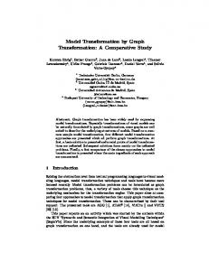
Figure 1: Process graph and BPEL control flow

The left part of Figure 1 shows a process graph. As we are interested in syntax transformations, we give the semantics of process graphs only in an informal manner. A process graph has at least one start event and can have multiple end events. Multiple start events represent mutually exclusive, alternative start conditions. End events have explicit termination semantics. This means that when an end event is reached, the complete process is terminated. Connectors represent split and join rules of type OR, XOR, or AND, as they are specified for YAWL [vdAtH05] or EPCs [MN05]. All of these elements are connected via arcs which may have an optional guard. Guards are logical expressions that can evaluate to true or false. If a guard of an arc from a connector node with type OR or XOR yields false, the target branch of the arc is not executed. If true, execution continues with the target function. After an XOR split, the logical expressions of guards of the subsequent arcs must be mutually exclusive. The right part of Figure 1 gives a BPEL control flow with similar semantics as the process graph. So-called structured activities can be nested in specific complex control flows. There are structured activities to define alternative start conditions (pick), parallel execution (flow), sequential execution (sequence), and conditional repetition (while). The switch activity for alternative branches is not depicted in Figure 1. Basic activities represent atomic elements of work. There are special basic activities to represent that nothing

is done (empty) or that the BPEL control flow is terminated (terminate). Within a flow activity, complex synchronization conditions can be specified via so-called links. Each link can have a transition condition, and each activity that is a target of links can include a join condition of the type OR, XOR, or AND. For BPEL control flow, we adopt the semantics defined in the BPEL specification [ACD+ 03].

2.2 Definition of Process Graphs To provide for a precise description of the transformation strategies, we formalize the syntax of process graphs and those aspects of BPEL that are relevant for a transformation of control flow. We define process graphs to be close to EPCs, and we adopt an EPC-like notation. The respective syntax elements provide the core of graph-based business process modelling languages, such as YAWL. Furthermore, AND and XOR connectors can easily be mapped to Petri nets, XPDL, or UML activity diagrams. Notation 1 (Predecessor and Successor Nodes) Let N be a set of nodes and A ⊆ N × N a binary relation over N defining the arcs. For each node n ∈ N , we define the set of predecessor nodes •n = {x ∈ N |(x, n) ∈ A}, and the set of successor nodes n• = {x ∈ N |(n, x) ∈ A}. Definition 1 (Process Graph PG) A process graph P G = (S, E, F, C, l, A, g) consists of four pairwise disjoint sets S, E, F, C, a mapping l : C → {AN D, OR, XOR}, a binary relation A ⊆ (S ∪ F ∪ C) × (E ∪ F ∪ C), and a mapping guard : A → expr such that: S denotes the set of start events. |S| ≥ 1 and ∀s ∈ S : |s•| = 1 ∧ |•s| = 0. E denotes the set of end events. |E| ≥ 1 and ∀e ∈ E : |•e| = 1 ∧ |e•| = 0. F denotes the set of functions. ∀f ∈ F : |•f | = 1 ∧ |f •| = 1. C denotes the set of connectors. ∀c ∈ C : |•c| = 1 ∧ |c•| > 1 ∨ |•c| > 1 ∧ |c•| = 1 The mapping l specifies the type of a connector c ∈ C as AN D, OR, or XOR. A defines the flow as a simple and directed graph. An element of A is called arc. Being a simple graph implies that ∀n ∈ (E ∪ F ∪ C) : (n, n) ∈ / A (no reflexive arcs) and that ∀x, y ∈ (E ∪ F ∪ C)} : |{(x, y)|(x, y) ∈ A}| = 1 (no multiple arcs). – The mapping guard specifies a guard for an arc a ∈ A. expr is a non-terminal symbol to represent a logical expression that defines the guard condition. If and only if this expression yields true, control is propagated to the node subsequent to the guard. Guards of arcs after XOR connector nodes have to be mutually exclusive. Guards are defined on A, however it is only arcs (c,n), where c ∈ C, l(c) 6= AN D and n ∈ E ∪ F ∪ C, that can be expressed as any logical expression. All other guard always yields true; e.g. a guard from an AND-split can never yield false and each function in a sequence is always executed. – – – – – –

Definition 2 (Transitive Closure) A∗ is the transitive closure of A. That is, if (n1 , n2 ) ∈ A∗ there is a path from n1 to n2 in the graph via some arcs of A.

2.3 Definition of BPEL Control Flow Definition 3 (BPEL Control Flow) A BPEL Control Flow BCF is a tuple BCF = (Seq, F low, Switch, W hile, P ick, Scope, Basic, Empty, T erminate, Link, de, jc, tc). BCF consists of pairwise disjoint sets Seq, F low, Switch, W hile, P ick, Scope, Basic, Empty, T erminate. The set Str = Seq ∪ F low ∪ Switch ∪ W hile ∪ P ick ∪ Scope is called structured activities, the set Bas = Basic ∪ Empty ∪ T erminate is called basic activities, and the set Act = Str ∪ Bas activities. Furthermore, BCF consists of a binary relation Link ⊆ Act × Act, a mapping de : S → P(A) \ ∅, a mapping jc : A → expr, and a mapping tc : Link → expr, such that – – – – – – –

– – – –

– –

Seq defines the set of BPEL sequence activities. F low defines the set of BPEL flow activities. Switch defines the set of BPEL switch activities. W hile defines the set of BPEL while activities. P ick defines the set of BPEL pick activities. Scope defines the set of BPEL scopes. Basic defines the set of BPEL basic activities without terminate and empty activities. As we are only interested in control flow, the distinction of various basic activities can be neglected here. Empty defines the set of BPEL empty activities. T erminate defines the set of BPEL terminate activities. Link defines a directed graph of BPEL links. These need not to be coherent, but acyclic, and not be connected across the borders of a while activity. The mapping de denotes a decomposition relation from structured activities to set of nested activities modelled as the power set P(A). de is a tree, i.e. there is no recursive decomposition. The mapping jc defines the join condition of activities. The mapping tc defines the transition condition of links.

Definition 4 (Join condition) The join condition, jc, on activities is defined as a jc : A → expr using operations such as ∧, ∨ and Y. For an activity x, where •x = {y1 , . . . , yn } including its predecessor in a structured activity, we use the shorthand AND, OR and XOR for the boolean expressions jc(x) = tc(y1 , x) ∧ . . . ∧ tc(yn , x) (AND) jc(x) = tc(y1 , x) ∨ . . . ∨ tc(yn , x) (OR) jc(x) = tc(y1 , x) Y . . . Y tc(yn , x) (XOR) Definition 5 (Subtree Fragment) Let Struct ⊆ Act × Act be relation with (a1 , a2 ) ∈ Struct if and only if a2 ∈ de(a1 ). Struct∗ is the transitive closure of Struct. This implies that a2 is nested in the subtree fragment of a1 . For the purpose of discussing control flow transformations, other BPEL elements than those included in the definition can be neglected. For details on BPEL semantics refer to [ACD+ 03]. Note that e.g. BPML has similar syntax elements with comparable semantics [Ark02]. Accordingly, the strategies discussed in the following section can also be applied to define transformations between BPML and process graphs.

2.4 Structural Properties of Process Graphs and BPEL Control Flow Various transformation choices are bound to certain structural properties of the input model. A process graph can be structured or unstructured and acyclic or cyclic. We define a process graph to be structured by the help of reduction rules. They provide not only a formalization of structuredness but also a means to define a transformation strategy from process graphs to BPEL control flow. Details on this will be explained in Section 4. Definition 6 (Structured Process Graph) A process graph PG is structured if and only if it can be reduced to a single node by the following reduction rules, otherwise it is unstructured. All the reduction rules describe a certain component that is part of the process graph and then how to replace it by a single function. 1. Sequence reduction: A sequence is a set of nodes f1 , . . . , fn ∈ F such that (f1 , f2 ), . . . , (fn−1 , fn ) ∈ A. P G is reduced by removing the sequence and adding a function fC representing the sequence: F := (F ∪ {fC }) \ {f1 , ..., fn }, A := (A ∪ {(x, fC ) | x ∈ •f1 } ∪ {(fC , x) | x ∈ fN •}) \ {(f1 , f2 ), ..., (fn−1 , fn )}. 2. Connector pair reduction: A connecter pair is composed of two connectors c1 , c2 ∈ C and functions c1 • ⊆ F such that |•c1 | = 1 (split), |c2 •| = 1 (join), l(c1 ) = l(c2 ) and c1 • = •c2 . Depending on the image of c1 and c2 under l we denote the blocks in the following ways. We call the connector pair an AND-block if l(c1 ) = and, OR-block if l(c1 ) = or and XOR-block if l(c1 ) = xor. PG is reduced by adding a function fC representing the connector pair: F := (F ∪ {fC }) \ c1 •, A := (A ∪ {(x, fC ) |x ∈ •c1 } ∪ {(fC , x)|x ∈ c2 •}) \ ({(x, c1 )|x ∈ •c1 } ∪ {(c1 , x)|x ∈ c1 •} ∪ {(x, c2 )|x ∈ •c2 } ∪ {(c2 , x)|x ∈ c2 •}) and C := C \ {c1 , c2 }. 3. XOR-loop reduction: An XOR-loop is composed of two connectors c1 , c2 ∈ C and functions c1 • ∩ • c2 , •c1 ∩ c2 • ⊆ F such that |c1 •| = 1 (join), |•c2 | = 1 (split) and either (1) c1 • = {c2 } and •c1 ∩ c2 • 6= ∅, (2) c1 • = •c2 and c2 ∈ •c1 , (3) c1 • = •c2 and •c1 ∩ c2 • 6= ∅ or (4) c1 • = {c2 } and c2 ∈ •c1 . We will refer to an XOR-loop of type (1) as a while-do loop, (2) as a repeat-until loop, (3) as a mixed loop and (4) as the empty loop. PG is reduced by removing the XOR-loop and adding a function fC representing the XOR-loop: F := (F ∪ {fC }) \ ((c1 • ∩ • c2 ) ∪ (•c1 ∩ c2 •)), A := (A∪{(x, fC )|x ∈ •c1 \c2 •}∪{(fC , x)|x ∈ c2 •\•c1 })\({(x, c1 )|x ∈ •c1 }∪ {(c1 , x)|x ∈ c1 •} ∪ {(x, c2 )|x ∈ •c2 } ∪ {(c2 , x)|x ∈ c2 •}) and C := C \ {c1 , c2 }. 4. Start-block: A start-block is composed of an XOR connector c and the set of start events S such that S = •c. PG is reduced by replacing the start-block by a function fC : S := ∅, F := F ∪ {fC }, A := (A ∪ {(fC , x)|x ∈ c•}) \ ({(x, c)|x ∈ •c} ∪ {(c, x)|x ∈ c•}) and C := C \ {c}. 5. End-block: An end-block is composed of an XOR connector c and the set of end events E such that E = c•. PG is reduced by replacing the end-block by a function fC : E = ∅, F := F ∪ {fC }, A := (A ∪ {(x, fC )|x ∈ •c}) \ ({(x, c)|x ∈ •c} ∪ {(c, x)|x ∈ c•}) and C := C \ {c}.

Definition 7 (Cyclic versus Acyclic Process Graph) Let F ∪ C be the set of functions and connectors of a process graph P G. If ∃n ∈ F ∪ C : (n, n) ∈ A∗, then P G is cyclic. If ∀n ∈ F ∪ C : (n, n) ∈ / A∗, then P G is acyclic. As a process graph is a simple graph, it holds that (n, n) ∈ / A (no reflexive arcs). But if (n, n) ∈ A∗, there must be a path from n to n via some further nodes n1 , ..., nm ∈ (E ∪ F ∪ C). Definition 8 (Structured BPEL Control Flow) A BPEL Control Flow BCF is structured if and only if its set Link = ∅. Otherwise BCF is unstructured. Furthermore, we define the point wise application of mapping functions which we need in algorithms for the transformation strategies. Definition 9 (Point Wise Application of Functions) If a function is defined as f : A → B then we extend the behavior to sets so that f (X) = ∪x∈X f (x), X ⊆ A.

3 BPEL Control Flow to Process Graph Transformation Strategies 3.1 Strategy 1: Flattening Before we present the transformation algorithms, we need to define the mapping function M that transforms a BPEL basic activity to a process graph function. Definition 10 (Mapping Function M) Let F be a set of functions of a process graph P G and Basic a set of basic activities of a BCF . The mapping M : Basic → F defines a transformation of a BPEL basic activity to a process graph function. Algorithm 1 Pseudo code for Flattening strategy procedure: Flattening(BCF ) 1: Struct ← Seq ∪ F low ∪ Switch ∪ W hile ∪ P ick ∪ Scope 2: S ← {s}; E ← {e}; F ← ∅; C ← ∅; A ← ∅ 3: root ← a, where a ∈ Struct ∧ @s ∈ Struct : de(s) = a 4: BCFtransform(root, s, e, P G) 5: for all (l1 , l2 ) ∈ Link do 6: A ← A ∪ {(c1 , c2 )} 7: guard(c1 , c2 ) = tc(l1 , l2 ) 8: end for 9: return P G The general idea of the Flattening strategy is to map BCF structured activities to respective process graph fragments. The nested BCF control flow then becomes a flat process graph without hierarchy. For this strategy, there are no prerequisites, both structured and unstructured BPEL control flow can be transformed according to this strategy. The advantage of Flattening is that the behavior of the whole BPEL process is mapped to one process graph. Yet, as a drawback the descriptive semantics of structured activities get

Algorithm 2 Pseudo code for BCFtransform procedure: BCFtransform(activity, pred, succ, P G) 1: if ∃(l1 , activity) ∈ Links then 2: C ← C ∪ {c1 }; l(c1 ) = jc(activity); A ← A ∪ {(pred, c1 )}; pred ← c1 3: end if 4: if ∃(activity, l2 ) ∈ Links then 5: C ← C ∪ {c2 }, l(c2 ) = OR; A ← A ∪ {(c2 , succ)}; succ ← c2 6: end if 7: if activity ∈ Seq then 8: P G ← BCFtransformSeq(activity, pred, succ, P G) 9: else if activity ∈ F low then 10: P G ← BCFtransformBlock(activity, pred, succ, AN D, P G) 11: else if activity ∈ Switch then 12: P G ← BCFtransformBlock(activity, pred, succ, XOR, P G) 13: else if activity ∈ W hile then 14: P G ← BCFtransformWhile(activity, pred, succ, P G) 15: else if activity ∈ P ick then 16: P G ← BCFtransformPick(activity, pred, succ, P G) 17: else if activity ∈ Scope then 18: P G ← BCFtransform(de(activity), pred, succ) 19: else if activity ∈ Basic then 20: F ← F ∪ {M (activity)}; A ← A ∪ {(pred, activity), (activity, succ)} 21: else if activity ∈ Empty then 22: A ← A ∪ {(pred, succ)} 23: else if activity ∈ T erminate then 24: E ← E ∪ {e}; A ← A ∪ {(pred, e)} 25: end if 26: return P G

lost. Such a transformation strategy is useful in a scenario where a BPEL process has to be communicated to business analysts. The algorithm for the Flattening strategy takes a BCF as input and returns a P G. It recursively traverses the nested structure of BPEL control flow in a top-down manner. This is achieved by identifying the root activity and invoking the BCFtransform(activity, predecessor, successor, partialResult) procedure (see Algorithm 1, line 4) which is reinvoked recursively on nested elements. The respective code is given in Algorithm 2. The first parameter activity represents the activity to be processed followed by the predecessor and successor node of the output process graph between which the nested structure is hooked in; i.e. predecessor and successor. For the root activity these are the start and end events s and e. The parameter partialResult is used to forward the partial result of the transformation to the procedure. In lines 5–8 links are mapped to arcs and respective join and split connectors around the activity are added. The BCF transf orm procedure (Algorithm 2) starts with checking whether the current activity serves as target or source for links. If so, respective connectors are added at the

beginning and the end of the current activity block. There are four sub-procedures to handle the five structured activities Seq, F low, Switch, W hile, and P ick. Here, it is assumed that P ick is only used to model alternative start events.1 The transformation of Scopes simply calls the procedure for its nested activity.2 T erminate is mapped to an end event. Moreover, Basic activities are mapped to functions using M and hooked in the process graph. Empty activities map to an arc between predecessor and successor nodes. The procedures BCF transf ormSeq, BCF transf ormBlock, BCF transf ormP ick, and BCF transf ormW hile generate the process graph elements that correspond to the respective BCF structured activities. BCF transf ormSeq connects all nested activities of a sequence with process graph arcs. Although not explicitly defined, this transformation requires an order defined on the nested activities. For each sub-activities the BCF transf orm procedure is invoked again. This is similar to BCF transf ormBlock. Here, a split and a join connector are generated. Depending on the label given as a fourth parameter the procedure can transform both Switch or F low. The BCF transf ormP ick replaces the start event of the process graph with one start event for each nested subactivity. Finally, the BCF transf ormW hile procedure generates a loop between an XOR join and an XOR split.

3.2 Strategy 2: Hierarchy-Preservation Many graph-based BPM languages allow to define hierarchies of processes. EPCs for example include hierarchical functions and process interfaces to model sub-processes. In YAWL tasks can be decomposed to sub-workflows. Process graphs can be extended to process graph schemas in a similar way to allow for decomposition. Definition 11 (Process Graph Schema PGS) A process graph schema P GS = {P G, s} consists of a set of process graphs P G and a mapping s : F → {∅, pg} with pg ∈ P G. The mapping s is called subprocess relation. It points from a function to a refining subprocess or, if the function is not decomposed, to the empty set. The relation s is a tree, i.e. there is no recursive definition of sub-processes. The general idea of the Hierarchy-Preservation strategy is to map each BCF structured activity to a process graph of a process graph schema. The nesting of structured activities is preserved as functions with subprocess relations. The algorithm can be defined in a top-down way similar to the Flattening strategy. Changes have to be defined for the transformation of structured activities as each is mapped to a new process graph. A prerequisite of this strategy is that the BCF is structured: links across the border of structured activities cannot the expressed by the subprocess relation. The advantage of the HierarchyPreservation strategy is that the descriptive semantics of structured activities can be preserved. Furthermore, such a transformation can correctly map the BPEL semantics of 1 In BPEL, P ick can be used at any place where the process waits for concurrent events. As we do not distinguish message-based and other basic activities, decisions are captured by a Switch in BCF . 2 Please note that Scopes play an important role in BPEL as a local context for variables, handlers, and also T erminate activities. In the algorithm we abstract from the fact that T erminate only terminates the current Scope but not the whole process.

Algorithm 3 Pseudo code for BCFtransformSeq procedure: BCFtransformSeq(activity, pred, succ, P G) 1: pre ← pred; 2: for all nested ∈ de(activity) do 3: A ← A ∪ {(pre, nested)} 4: P G ← BCFtransform(nested, pre, next(nested), P G) 5: pre ← nested 6: end for 7: nested ← last(de(activity)) 8: A ← A ∪ {(pre, nested), (nested, succ)} 9: P G ← BCFtransform(nested, pre, succ, P G) 10: C ← C ∪ {c1 , c2 } 11: return P G Algorithm 4 Pseudo code for BCFtransformBlock procedure: BCFtransformBlock(activity, pred, succ, label, P G) 1: decomp ← de(activity) 2: C ← C ∪ {c1 , c2 } 3: l(c1 ) ← label; l(c2 ) ← label 4: A ← A ∪ {(pred, c1 ), (c2 , succ)} 5: for all current ∈ decomp do 6: P G ← BCFtransform(current, c1 , c2 , P G) 7: end for 8: return P G Algorithm 5 Pseudo code for BCFtransformPick procedure: BCFtransformPick(activity, pred, succ, P G) 1: decomp ← de(activity) 2: S ← ∅; A ← A \ {(s, y)|s ∈ S} 3: C ← C ∪ {c}; l(c) = XOR; 4: for all current ∈ decomp do 5: S ← S ∪ {scurrent } 6: sL ← {(l1 , l2 ) ∈ Links|l1 = current} 7: P G ← BCFtransform(current, s, c, P G) 8: end for 9: return P G Algorithm 6 Pseudo code for BCFtransformWhile procedure: BCFtransformWhile(activity, pred, succ, P G) 1: decomp ← de(activity) 2: C ← C ∪ {c1 , c2 } 3: l(c1 ) = XOR; l(c2 ) = XOR 4: A ← A ∪ {(pred, c1 ), (c1 , c2 ), (c2 , succ)} 5: P G ← BCFtransform(decomp, c2 , c1 , P G) 6: return P G

T erminate activities that are nested in Scopes. As a drawback, the model hierarchy has to be navigated in order to understand the whole process. This strategy might be useful in a scenario where process graphs have to be mapped back to BPEL structured activities.

3.3 Strategy 3: Hierarchy-Maximization One disadvantage of Strategy 2 is that it is bound to structured BPEL. The HierarchyMaximization Strategy aims at preserving as much hierarchy as possible with also being applicable to any BPEL control flow – anyway if structured or unstructured. The general idea of the strategy is to map those BCF structured activities s to subprocess hierarchies if there are no links nested that cross the border of s. Accordingly, this strategy is not subject to any structural prerequisites. The advantage is that as much structure as possible is preserved. Yet, the logic of both Strategy 1 and Strategy 2 need to be implemented.

4 Process Graph to BPEL Control Flow Transformation Strategies 4.1 Strategy 1: Element-Preservation In this section we will describe the first strategy for going from process graphs to BCF . The following Definitions 12 (Annotated Process Graph) and 13 (Annotated Process Graph Node Map) are also relevant of further strategies. Before we go through the strategies we will make some definitions where we introduce the notion of an annotated process graph to ease the notation in strategy. Definition 12 (Annotated Process Graph) Let AP G = (S, E, F, C, l, A, B) define an annotated graph, where S, E, F, C and l are defined as Definition 1. We define A and B as – A is a flow relation on the nodes in PG, A = (S ∪ F ∪ C ∪ B) × (E ∪ F ∪ C ∪ B). – B is a node in PG that holds an annotation in BCF. One could think of the set B in the annotated graph, Definition 12, as the set of already translated parts of the process graph. Definition 13 shows how to translate the nodes in an annotated process graph. The general idea of this strategy is to map all process graph elements to a F low and map arcs to Links. In particular, start events are mapped to Basic,3 function are mapped to elements of Basic, and connectors are mapped to elements of Empty, and end events are translated to elements of T erminate. M defines the identity on BPEL constructs. Definition 13 (Annotated Process Graph Node Map) Let M define a mapping: E ∪ S ∪ 3 As a consequence, all alternative start branches are activated when the process is started. Specific transition conditions could be defined to have only one branch being activated. In the algorithm we abstract from this issue.

F ∪ C ∪ B → Basic ∪ Empty ∪ T erminate ∪ B and M is defined as  Empty(x), if x ∈ C;    Basic(x), if x ∈ F ∪ S; M (x) = T erminate(x), if x ∈ E;    x, if x ∈ B. an injective translation from the nodes in the graph to activities in BPEL. It is a prerequisite of this strategy that the process graph needs to be acyclic, i.e. (x, x) ∈ / A∗, because the BPEL F low structured activity uses dead path elimination to synchronize parallel paths [ACD+ 03] and dead path elimination works only for acyclic processes. The advantage of the Element-Preservation strategy is that it is simple to implement and the resulting BPEL will be very similar to the original process graph since there is a oneto-one correspondence between the nodes. As a drawback, the resulting BPEL control flow includes more elements than actually needed: connectors are explicitly translated to empty activities in BPEL instead of join condition on nodes. This means that the BPEL code might have a lot of nodes which simply act as synchronization points. Furthermore, the resulting BPEL might be more difficult to understand than if structured activities, such as the Switch, where chosen to represent some part of the translated graph. If the BPEL code is used in a scenario where readability is important, then it should be applied only for small process graphs since all elements of the process graph are mapped to BCF . Algorithm 7 Pseudo Code for Element-Preservation strategy procedure: Element-Preservation(P G) 1: Empty ← M (C) 2: Basic ← M (F ∪ S) 3: T erminate ← M (E) 4: F low ← f low 5: de(f low) ← Empty ∪ Basic ∪ T erminate 6: Link ← ∅ 7: for all (x, y) ∈ A do 8: Link ← Link ∪ (M (x), M (y)) 9: end for   AN D, | • M −1 (x)| > 1 ∧ l(M −1 (x)) = and; XOR, | • M −1 (x)| > 1 ∧ l(M −1 (x)) = xor; 10: jc(x) =  OR, otherwise. 11: tc(x, y) = guard(M −1 (x), M −1 (y)) 12: return(BCF ) The algorithm for the Element-Preservation strategy takes a process graph as input and generates a respective BCF as output. The Algorithm 7 applies the map M as defined in Definition 13 in lines 1–3. Then, a flow element is added that nests all other activities (lines 4–5). For each arc in the process graph between two nodes a link is added in the BCF between the corresponding two BCF nodes (lines 6–9). The join condition of activities is determined from their corresponding node in the process graph. If it is a connector it will

get a similar join condition, i.e. AND for and, OR for or and XOR for xor. Other nodes will get an OR join condition (line 10). If two nodes are connected by a guarded arc then this guard will also be present in the BPEL (line 11).

4.2 Strategy 2: Element-Minimization This strategy simplifies the generated BCF of strategy 1. The general idea is to remove the empty activities that have been generated from connectors and instead represent splitting behavior by transition conditions of links and joining behavior by join conditions of subsequent activities. As a prerequisite the process graph needs to be acyclic, i.e. (x, x) ∈ / A∗, in order to make dead path elimination of BPEL work. The advantage of the resulting BCF specification is, at least to a greater extent than strategy 1, that it is in the spirit of BPEL Flow, since it removes empty activities generated from connectors. As a drawback, it is less intuitive to identify correspondences between the process graph and the generated BCF specification. This strategy should be used in scenarios where the resulting BPEL code needs to be compact. This might be the case when performance of the BPEL process matters. In contrast to strategy 1, the amount of nodes is decreased since all empty activities translated from connector nodes are skipped . Algorithm 8 Pseudo code for Element-Minimization strategy procedure: Element-Minimization(P G) 1: BCF ← Element-Preservation(P G) 2: while ∃x ∈ Empty : M −1 (•x) ∩ C = ∅ do 3: Link ← Link ∪ {(y1 , y2 ) | y1 ∈ •x ∧ y2 ∈ x•} 4: for all y µ ∈ x• do ½ ¶ jc(y 0 ), y 0 6= y; 5: jc ← jc0 (y 0 ) = jc(y 0 ) ∧ jc(x), otherwise. 6: end for 7: Link ← Link \ ({(x, y) | y ∈ x•} ∪ {(x, y) | y ∈ •x}) 8: Empty ← Empty \ {x} 9: end while 10: return(BCF ) The algorithm translates a P G into a BCF using Algorithm 7 (line 1). Then, there is a loop iterating over all empty activities that have been generated from connectors (line 2) and do not have other translated connector nodes as input links. Finally all translated connector nodes will be removed. For each empty activity x, the nodes having a link to it, are connected to nodes having a link from it. Then, the join conditions of the activities subsequent to x need to be updated. The join condition of an activity is the old join condition it had, before removing x, in conjunction with the join condition of x (lines 4– 6). Lines 7–9 defines the actual removal of x. This involves removing all link relations that x occurs in and removing x from the set of Empty activities.

4.3 Strategy 3: Structure-Identification The general idea of this transformation strategy is to identify structured activities in the process graph and apply mappings that are similar to the reduction rules given in Definition 6 on them. As a prerequisite the process graph needs to be structured according to Definition 6. The advantage of this strategy is that all control flow is translated to structured activities. For understanding the resulting code this is the best strategy since it reveals the structured components of the process graph. As a drawback the relation to the original process graph might not be intuitive to identify. This transformation strategy is appropriate in a scenario when the BCF is to be edited by a BPEL modeling tool or, generally, when understanding the control flow of the process graph is important. Our algorithm uses the reduction rules of Definition 6, but instead of substituting a pattern with a function it is replaced by an annotated node containing the BPEL translation of the process graph fragment. This means, in reducing the process graph we generate an annotated process graph that finally includes only one single annotated node. A single function is mapped to Basic in the resulting BCF , whereas annotated nodes are mapped to the set which their annotation is a member of; e.g. Switch if a Switch annotation. Each of the rules identifies structure that has an equivalent representation in BPEL as follows: – A sequence of elements is translated to a BCF sequence with activities in the same order as nodes of the process graph sequence. – An AND-block is translated to a flow in the BCF . The nodes of the AND-block are translated to nested activities of the flow. – An OR-block is translated to a flow in the BCF . The nodes of the OR-block are translated to nested activities of the flow with an additional empty activity. This points to each alternative branch and transition conditions are used to activate only a subset of branches. Notice that this translation makes the BCF unstructured. – An XOR-block is translated to a switch in the BCF . Each branch of the XOR-block is mapped to a nested activity of the switch including the respective guard. – A mixed loop has no direct representation in the BCF . As the rule in Definition 6 state the graph has the structure c1 • = {a1 }, •c1 ∩ c2 • = {a2 , . . . , an }. The condition to leave the loop is cond, i.e. the boolean expression (Yx∈A guard(x)) ∧ ¬(Yx∈B guard(x)), A = {(c2 , x)|x ∈ •c1 ∩ c2 •} and B = {(c2 , x)|x ∈ / •c1 ∩ c2 •}. However, since exactly one of the arcs from an XOR connector node is true at a time the boolean expression can be reduced to both the left and the right part in the conjunction. Guards in PG are mapped to transition conditions in the BF C. The mixed loop can be mapped to the following BPEL pseudo code: 1: assign(continueLoop,true); 2: while(continueLoop) { 3: M(a1); 4: switch { 5: case cond: assign(continueLoop,false); 6: case tc(c2,a2)): M(a2); 7: ... 8: case tc(c2,an)): M(an); 9: } 10:}

– A while-do loop is translated into a while activity with a switch inside it. It is mapped as the mixed loop with the difference that lines 1, 3, and 5 are omitted and the condition, cond, for looping replaces the continueLoop in line 2. – A repeat-until loop has no direct representation in the BCF . It is mapped in a similar way as the mixed loop – lines 6 through 8 in the pseudo code are omitted. – An empty loop is translated to an empty activity. – A start-block is mapped to a Pick containing empty activities for each branch. – An end-block is translated to a respective AND-, OR-, or XOR-block with each branch followed by a terminate activity. Algorithm 9 Pseudo code for Structure-Identification strategy procedure: Structure-Identification(P G) 1: AP G ← (S, E, F, C, l, A, ∅) 2: while |F ∪ C ∪ B| > 1 do 3: AP G0 ← match(AP G) {Using rules in Definition 6} 4: b ← translate(AP G0 ) {Using the described translations above} 5: Reduce APG substituting APG’ with b {Using rules in Definition 6} 6: end while 7: return(BCF ) Algorithm 9 describes the Structure-Identification transformation strategy. Line 1 initializes the annotated process graph. After that, a loop is iterated until the annotated process graph is reduced down to one activity. The reduction rules of Definition 6 are used to substitute components of the process graph by corresponding BCF structured activities in the same way as the function fC substituted components in Definition 6.

4.4 Strategy 4: Structure-Maximization The general idea of this strategy is to apply the reduction rules of the Structure-Identification strategy as often as possible to identify a maximum of structure. The remaining annotated process graph is then translated following the Element-Preservation or ElementMinimization strategy. The advantage of this strategy is that it can be applied for arbitrary unstructured process graphs as long as its loops can be reduced via the reduction rules of Definition 6. Still this strategy is also not able to translate arbitrary cycles, i.e. cycles with multiple entrance and/or multiple exit points. A drawback of this strategy is that both the Structure-Identification strategy and at least the Element-Preservation strategy needs to be implemented. The strategy could be used in scenarios where models have to be edited by a BPEL modeling tool.

5 Case Studies 5.1 Visualizing BPEL as EPC Models In a research project [MZ05], we defined a conceptual mapping from BPEL to EPCs and implemented the transformation as a script that generates BPEL from EPC Markup Language (EPML) [MN05]. The idea was to reuse experiences from this project in a later conceptualization of an EPC-driven development approach for BPEL (see [ZM05]). In this project, we chose for a Flattening transformation strategy as it would allow to visualize BPEL behavior in one EPC model. Such an EPC model could be used to discuss processes with business analysts who are more familiar with EPCs. In the context of control flow there was only one problem with this strategy: the mapping of terminate activities. EPC end events define implicit termination semantics, i.e. process instances are only terminated when all active branches have completed. In EPCs there is no concept that allows to terminate activities or the whole process instance. This is a difference to process graphs P G as defined in this paper and poses problems with the mapping of terminate activities and scopes. An extension to EPCs called yEPCs is needed to capture the semantics of terminate via a cancellation concept similar to YAWL [MNN05]. Scopes with nested terminate activities can then be mapped to cancellation areas. Beyond the transformation of BPEL control flow also BPEL partner links and variables can be mapped to EPML elements. For each partner link referenced in a invoke, receive, reply, or pick activity a participant element is generated. For each activity interacting with variables a data field element is created. These include the four previously mentioned activities that store the content of received messages in variables or send messages built from variables, assign activities that change variable values, throw activities if they write to fault variables, and wait activities because time is also considered to reading the current time. An open issue is the representation of handlers in EPCs. At least event handlers could be represented as parallel threads to the main process. If the BPEL process includes several scopes, the interaction of usual control flow and fault and compensation handlers becomes soon very complex. Therefore, we decided to not include handlers in an EPC model that is meant to visualize BPEL control flow. In conclusion, the Flattening transformation strategy was easy to adopt for this project. The mapping of the terminate activity to EPCs could be defined using the yEPC extension to EPCs.

5.2 BPEL Export of UML-based Workflow Designer In an industry project, we designed a BPEL export filter for a workflow designer that uses a graph-oriented notation based on UML activity diagrams including product-specific extensions. In essence, we followed the Element-Preservation strategy and deviated in order to capture differences between process graphs and the UML activity diagram variant of the workflow designer. These deviations related to start and end events, split elements, and a two-level modelling concept. In contrast to process graphs as defined in this paper, models built by the workflow designer have exactly one start node and end nodes with implicit termination semantics. As they do not need to be represent in the flow element, we

decided not to transform them to BPEL. Accordingly, also arcs connected with start and end nodes are not mapped to BPEL links. The workflow designer offers two split elements that have semantics comparable to an XOR split; these are switch nodes (two alternatives) and decision nodes (multiple alternatives). We decided to map both of these elements to a BPEL switch that includes empty elements for each alternative that serves as a source for a link to the subsequent activity. This design has been chosen in order to easier distinguish different types of splits when the exported BPEL is re-imported. Furthermore, the workflow designer offers a two-level modelling approach: step nodes similar to process graph functions have to be specified by a sequence of one or multiple step actions. Step nodes are part of the UML model, step actions have no visual representation. As a consequence, we map step nodes to BPEL sequences that nest further BPEL activities corresponding to the semantics of the step actions. A problem has been the mapping of specific concepts of the workflow designer. These include sub-workflow elements, step actions, and properties. For sub-workflows, we decided to map them to BPEL scopes and a nested invoke. This allows to define the input parameters of the sub-workflow as local variables in the scope and to represent the invocation of the sub-process via a BPEL invoke. Furthermore, all visual elements of the workflow designer can have additional properties, some like time-out conditions and escalation have even influence on control flow. We defined a special XML namespace for these properties and included them as attributes in the respective BPEL activity. Finally, we had to map step actions contained in the step nodes to BPEL basic activities. Step actions are defined in an abstract class, which is customized in a number of different possible actions, such as e.g. setting a variable, inline Java code, or mail sending. To map these steps, we first defined a generic mapping operation to BPEL in the abstract step action class which is used when no special class overrides the operation. In this case, a BPEL invoke is written to the output, containing the name of the step as partner link. We also defined mappings for a number of concrete step actions. For instance, in the step action for invoking a form-based input, the partner link is set to the application receiving the form-based input. The inline Java code step action is transformed to a BPELJ snippet. The rule checking step action is mapped to a BPEL empty activity that includes a rule attribute. The variable setting step action is mapped to a BPEL assign activity. In conclusion, our transformation strategies have helped us to find a systematic, initial approach and process for the transformation of the workflow designer’s notation to BPEL. They are also useful for explaining design decisions. In a real-world industry product, however, there are proprietary extensions, such as step actions or properties, and model elements with further semantics, such as sub-workflows, which are not captured by process graphs as defined in this paper. These require deviations from the general transformation strategies. As future work, we plan to extend the transformation to a StructureMaximization strategy in order to be able to export cyclic models of the workflow designer, too.

6 Related Work A lot of work exists on transformation between BPEL and other process languages. A large branch of such work is dedicated to model-driven development of executable BPEL process definitions. In [Gar03] a BPM-specific profile of UML is used to generate BPEL code. Yet, the aim is rather to prove the feasibility of such an approach than the discussion of different transformation alternatives. From the paper, it is neither clear which strategy the author chooses nor the criteria that drive the design decision. The only hint on the mapping of control flow is that BPEL sequence and BPEL flow are mentioned. Presumably, the author uses an Element-Preservation strategy and maps sequences to BPEL sequence. In [HH04] UMM, which is a UML profile that captures the concept of ebXML’s choreography language BPSS, is translated to BPEL. The aim of the paper is to show how UMM business transactions can be mapped to BPEL. The authors present output of the transformation that includes BPEL structured activities. Yet, control flow mapping is not discussed in the paper. In [MH05] the new choreography language WS-CDL is used to generate BPEL stubs for each participating party of the choreography. As WS-CDL also offers block-oriented control flow primitives, there are no graph-to-block transformations needed. The BPMN specification [Whi04] comes along with a proposal for a mapping to BPEL. As BPMN is a graph-oriented BPM language similar to process graphs, the strategies of Section 4 can be applied. The subsection 6.17 of BPMN spec presents a mapping that is close to the Structure-Identification strategy proposed in this paper. The authors introduce so-called conceptual tokens to identify structure. Yet, the mapping is given rather in prose, a precise algorithm and a definition of required structural properties is missing. A conceptual mapping from EPCs to BPEL is presented in [ZM05]. The authors pragmatically choose a transformation based on the Element-Preservation strategy in order to support EPC-driven development of BPEL processes that is easy to implement. Further strategies are not considered. In [vdAJL05] a Workflow-net-based modeling approach for BPEL including a respective transformation is presented. Similar to the Structure-Identification strategy, Workflow nets are reduced by matching components that are equivalent to BPEL structured activities such as switch and pick. The StructureIdentification strategy has been chosen in order to generate readable BPEL template code and not executable BPEL processes. In [BBCT04] a model-driven development approach for generating BPEL skeletons from self-serv models is presented. As the focus of this research is rather on message interaction represented as state charts conversation protocols, our control flow transformation strategies are not applicable. A second branch of research is related to conceptual mappings in order to better understand BPEL behavior and its relation to other BPM languages. In [MLPC04] transformation algorithms from BPEL to BPML and from BPML to BPEL are discussed. The motivation of this research is to better understand the similarities and differences of both languages. Yet, as both BPEL and BPML share similar control flow primitives, there is no need to map between structured activities and graph-oriented control flow. In [HSS05, vdAJL05] a transformation from BPEL to Petri Nets is presented in order to give BPEL formal semantics. The authors use a Flattening strategy to generate a Petri Net that covers BPEL behavior including exceptional behavior. The generated Petri Net is used for formal static analysis of the BPEL model.

7 Conclusion and Future Work In this paper, we addressed the problem of transformations between graph-oriented and block-oriented BPM languages. In order to discuss such transformations in a general way, we defined process graphs as an abstraction of graph-oriented BPM languages and BPEL control flow as an abstraction of BPEL that shares most of its concepts with blockoriented languages like BPML. Our major contribution is the identification of different transformation strategies between the two BPM modelling paradigms and their specification as pseudo code algorithms. In particular, we identify the Flattening, HierarchyPreservation, and the Hierarchy-Maximization strategy for transformations from BPEL control flow to process graphs. In the other direction we identify Element-Preservation, Element-Minimization, Structure-Identification, and Structure-Maximization strategy. We present the applicability of these strategies in two case studies and discuss related work on BPEL transformations in the light of the strategies. As such, the strategies provide a useful generalization of many current X-to-BPEL and BPEL-to-Y papers not only for identifying design alternatives but also for discussing design decisions. In future research, we aim to conduct further case studies in order to identify how aspects that are not captured by process graphs and BPEL control flow can be addressed in a systematic way. Another issue is the upcoming new version of BPEL which is expected to be issued as a standard in the beginning of 2006. It will be interesting to discuss in how far that new version simplifies or complicates the mapping to and from graph-oriented BPM languages.

References [ACD+ 03]

T. Andrews, F. Curbera, H. Dholakia, Y. Goland, J. Klein, F. Leymann, K. Liu, D. Roller, D. Smith, S. Thatte, I. Trickovic and S. Weerawarana. Business Process Execution Language for Web Services, Version 1.1. Specification, BEA Systems, IBM Corp., Microsoft Corp., SAP AG, Siebel Systems, 2003.

[Ark02]

A. Arkin. Business Process Modeling Language (BPML). Spec., BPMI.org, 2002.

[BBCT04]

Karim Ba¨ına, Boualem Benatallah, Fabio Casati and Farouk Toumani. ModelDriven Web Service Development. In Anne Persson and Janis Stirna, editors, CAiSE, volume 3084 of Lecture Notes in Computer Science, pages 290–306. Springer, 2004.

[Gar03]

Tracy Gardner. UML Modelling of Automated Business Processes with a Mapping to BPEL4WS. In Proceedings of the First European Workshop on Object Orientation and Web Services at ECOOP 2003, 2003.

[HH04]

Birgit Hofreiter and Christian Huemer. Transforming UMM Business Collaboration Models to BPEL. In Robert Meersman, Zahir Tari and Angelo Corsaro, editors, OTM Workshops, LNCS 3292, pages 507–519, 2004.

[Hol04]

David Hollingsworth. The Workflow Handbook 2004, chapter The Workflow Reference Model: 10 Years On, pages 295–312. Workflow Management Coalition, 2004.

[HSS05]

Sebastian Hinz, Karsten Schmidt and Christian Stahl. Transforming BPEL to Petri Nets. In Proceedings of BPM 2005, LNCS 3649, pages 220–235, 2005.

[KNS92]

G. Keller, M. N¨uttgens and A. W. Scheer. Semantische Prozessmodellierung auf der Grundlage “Ereignisgesteuerter Prozessketten (EPK)”. Heft 89, Institut f¨ur Wirtschaftsinformatik, Saarbr¨ucken, Germany, 1992.

[MH05]

Jan Mendling and Michael Hafner. From Inter-Organizational Workflows to Process Execution: Generating BPEL from WS-CDL. In Robert Meersman, Zahir Tari and Pilar Herrero, editors, Proceedings of OTM 2005 Workshops, LNCS 3762, pages 506–515, 2005.

[MLPC04]

Jinyoung Moon, Daeha Lee, Chankyu Park and Hyunkyu Cho. Transformation Algorithms between BPEL4WS and BPML for the Executable Business Process. In Proc. of WETICE 2004, pages 135–140. IEEE Computer Society, 2004.

[MN05]

Jan Mendling and Markus N¨uttgens. EPC Markup Language (EPML) - An XMLBased Interchange Format for Event-Driven Process Chains (EPC). Technical Report JM-2005-03-10, WU Wien, Austria, 2005.

[MNN04]

Jan Mendling, Markus N¨uttgens and Gustaf Neumann. A Comparison of XML Interchange Formats for Business Process Modelling. In F. Feltz, A. Oberweis and B. Otjacques, editors, Proceedings of EMISA 2004, LNI 56, pages 129–140, 2004.

[MNN05]

Jan Mendling, Gustaf Neumann and Markus N¨uttgens. Yet Another Event-Driven Process Chain. In Proceedings of BPM 2005, LNCS 3649, pages 428–433, 2005.

[MZ05]

J. Mendling and J. Ziemann. EPK-Visualisierung von BPEL4WS Prozessdefinitionen. In Proc. of Workshop on Software Reengineering, Germany, 2005.

[RtHEvdA05] Nick Russell, A.H.M. ter Hofstede, D. Edmond and Wil M.P. van der Aalst. Workflow Data Patterns: Identification, Representation and Tool Support. In Proc. of the 24th International Conference on Conceptual Modeling (ER 2005), LNCS, 2005. [Tha01]

S. Thatte. XLANG. Specification, Microsoft Corp., 2001.

[vdA97]

W. M. P. van der Aalst. Verification of Workflow Nets. In Pierre Az´ema and Gianfranco Balbo, editors, Application and Theory of Petri Nets, LNCS 1248, pages 407–426, 1997.

[vdAJL05]

Wil M.P. van der Aalst, Jens Bæk Jørgensen and Kristian Bisgaard Lassen. Let’s Go All the Way: From Requirements via Colored Workflow Nets to a BPEL Implementation of a New Bank System. In R. Meersman and Z.Tari, editors, Proceedings of CoopIS/DOA/ODBASE 2005, Agia Napa, Cyprus, LNCS 3760, pages 22–39, 2005.

[vdAtH05]

Wil M. P. van der Aalst and Arthur H. M. ter Hofstede. YAWL: Yet Another Workflow Language. Information Systems, 30(4):245–275, 2005.

[vdAtHKB03] Wil M. P. van der Aalst, Arthur H. M. ter Hofstede, Bartek Kiepuszewski and Alistair P. Barros. Workflow Patterns. Distributed and Parallel Databases, 14(1):5–51, July 2003. [Whi04]

S. A. White. Business Process Modeling Notation. Specification, BPMI.org, 2004.

[Wor02]

Workflow Management Coalition. Workflow Process Definition Interface – XML Process Definition Language. Document Number WFMC-TC-1025, October 25, 2002, Version 1.0, Workflow Management Coalition, 2002.

[ZM05]

J. Ziemann and J. Mendling. EPC-Based Modelling of BPEL Processes: a Pragmatic Transformation Approach. In Proceedings of MITIP 2005, Italy, 2005.