TRANSFORMATIONAL PLANNING OF REACTIVE ... - Semantic Scholar

TRANSFORMATIONAL PLANNING OF REACTIVE BEHAVIOR Drew McDermott YALEU/CSD/RR #941 December, 1992 This work was supported by the Defense Advanced Research Projects Agency, contract number N00014-91-J-1577, administered by the Oce of Naval Research.

Transformational Planning of Reactive Behavior Drew McDermott

Abstract

Reactive plans are plans that include steps for sensing the world and coping with the data so obtained. We investigate the application of AI planning techniques to plans of this sort in a simple simulated world. To achieve fast reaction times, we assume that the agent starts with a default reactive plan, while the planner attempts to improve it by applying plan transformations, thus searching through the space of transformed plans. When the planner has what it believes to be a better plan, it swaps the new plan into the agent's controller. The plans are written in a reactive language that allows for this kind of swapping. The language allows for concurrency, and hence, truly \nonlinear" plans. The planner evaluates plans by projecting them, that is, generating scenarios for how execution might go. The resulting projections give estimates of plan values, but also provide clues to how the plan might be improved. These clues are unearthed by critics that go through the scenario sets, checking how the world state and the agent state evolved. The critics suggest plan transformations with associated estimates of how much they will improve the plan. Plan transformations must be able to edit code trees in such a way that the changes are orthogonal and reversible whenever possible. The system has been tested by comparing the performance of the agent with and without planning. Preliminary results allow us to conclude that the planner can be fast and directed enough to generate improved plans in a timely fashion, and that the controller can often cope with a sudden shift of plan.

1

Table of Contents

1 Overview . . . . . . . . . . . . . . . . . . 1.1 Agent Architecture . . . . . . . . . . . 1.2 An Example Transformation . . . . . . . 1.3 Transformation Audit Trails . . . . . . . 1.4 Planning and Execution . . . . . . . . . 1.5 Related Work . . . . . . . . . . . . . . 2 The Reactive Plan Language . . . . . . . . . 2.1 Perception . . . . . . . . . . . . . . . 2.2 Code Trees and Task Networks . . . . . . 2.3 Concurrency . . . . . . . . . . . . . . 3 The Projector . . . . . . . . . . . . . . . . 3.1 The Timeline . . . . . . . . . . . . . . 3.2 Action-Projection Rules . . . . . . . . . 3.3 Keeping Track of the Agent's Projected State 4 The Planner . . . . . . . . . . . . . . . . 4.1 The Life Cycle of Bugs . . . . . . . . . . 4.2 Bug Penalties . . . . . . . . . . . . . . 5 The World . . . . . . . . . . . . . . . . . 5.1 Some RPL Plans and Plan Models . . . . . 6 Bugs and Transformations . . . . . . . . . . 6.1 Utilities . . . . . . . . . . . . . . . . 6.2 Giving Up . . . . . . . . . . . . . . . 6.3 Scheduling . . . . . . . . . . . . . . . 6.4 Protection Violation . . . . . . . . . . . 6.5 Carrying Things in Boxes . . . . . . . . . 6.6 Declarative Goals . . . . . . . . . . . . 7 Results . . . . . . . . . . . . . . . . . . 8 Conclusions and Future Work . . . . . . . . . 9 References . . . . . . . . . . . . . . . . .

. . . . . . . . . . . . . . . . . . . . . . . . . . . . .

2

. . . . . . . . . . . . . . . . . . . . . . . . . . . . .

. . . . . . . . . . . . . . . . . . . . . . . . . . . . .

. . . . . . . . . . . . . . . . . . . . . . . . . . . . .

. . . . . . . . . . . . . . . . . . . . . . . . . . . . .

. . . . . . . . . . . . . . . . . . . . . . . . . . . . .

. . . . . . . . . . . . . . . . . . . . . . . . . . . . .

. . . . . . . . . . . . . . . . . . . . . . . . . . . . .

. . . . . . . . . . . . . . . . . . . . . . . . . . . . .

. . . . . . . . . . . . . . . . . . . . . . . . . . . . .

. . . . . . . . . . . . . . . . . . . . . . . . . . . . .

. . . . . . . . . . . . . . . . . . . . . . . . . . . . .

. . . . . . . . . . . . . . . . . . . . . . . . . . . . .

. . . . . . . . . . . . . . . . . . . . . . . . . . . . .

. . . . . . . . . . . . . . . . . . . . . . . . . . . . .

. . . . . . . . . . . . . . . . . . . . . . . . . . . . .

. . . . . . . . . . . . . . . . . . . . . . . . . . . . .

. . . . . . . . . . . . . . . . . . . . . . . . . . . . .

. . . . . . . . . . . . . . . . . . . . . . . . . . . . .

. . . . . . . . . . . . . . . . . . . . . . . . . . . . .

. . . . . . . . . . . . . . . . . . . . . . . . . . . . .

. . . . . . . . . . . . . . . . . . . . . . . . . . . . .

. 2 . 6 . 8 11 12 13 15 15 17 20 23 24 29 31 35 36 39 40 42 52 52 54 54 57 60 62 63 66 68

1 Overview All robots are controlled in some way, but not all robots reason about their controllers. When a robot designs or debugs a part of its own controller, we can call that part its plan. The rationale for this choice of terms is that reasoning about control almost always requires thinking about how alternative controllers would react to future events, and thinking about the future is the essence of planning (McDermott 1992b). A robot has no need of a plan if its controller can be designed o-line by humans. But, as in other areas, there is a clear need for automation here, to allow for faster and more reliable reprogramming of robots by getting the robots to do it themselves on the spot in response to the current context. When a mobile robot is given one more errand to run, it should be able to gure out for itself at what point in its schedule to insert the new job. A plan is reactive if it speci es how an agent is to react to sensory data at run time. A nonreactive plan corresponds to what is traditionally called \open-loop" control, which is feasible only when the agent's controller has an excellent model of the world. We will not assume such a model here. The agent's information about the state of the world can be incomplete or even wrong. The world can change independent of what the agent does. The research reported here is an attempt to get a computer to plan the reactive control of a robot. The robot is to be given jobs such as nding a big white cube near location h3; 5i and putting it in the big black box last seen near location h10; 12i. It may be given several jobs at once, not necessarily simultaneously. It attempts to nd the quickest way to accomplish its current list of jobs successfully. The question arises how we specify jobs to the robot. One way would be to describe a state of aairs, the job then consisting of bringing it about. However, we opt for a somewhat dierent formulation. A job is a program. What the robot has to do is carry it out. If the program nishes in the normal way, we count the robot as successful. However, if the program should explicitly fail, then the robot has failed to carry out its assignment. The planner can play it safe, and just execute the programs as they are given to it, in which case we expect them to have a good chance of succeeding, albeit ploddingly. However, the planner can often improve the plan by applying plan transformations to it. The resulting plan is supposed to perform better (more eciently and robustly), but it may now contain new bugs due to interactions of pieces of the plan that have been thrown together. Sometimes the plan, even with bugs, still works better than the original, because it is designed to cope to a degree with unexpected contingencies. But the planner continues to transform it in the hope of eliminating all bugs and ineciencies. Throughout this process, the agent controller uses the best plan the planner has found so far. There is no lag between a planning phase and an execution phase. The design of the notation in which the robot's programs are written is critical. On the one hand, it must be exible enough to control a realistic robot | even when several programs are run simultaneously in a changing and uncertain world. On the other, it must be transparent enough so that the planner can reason about the execution of plans and see ways to improve them. The notation I am developing, called RPL, for Reactive Plan Language (McDermott 1991b), is an eort to meet both these requirements. It is still 3

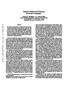
evolving, but the burden of this paper is to argue that it meets them to some degree. The resulting notation is more like a robot programming langauge than a classical plan language. It contains local variables, loops, multiple processes, interrupts, and several other features. Its syntax, of course, is Lisp-like. The planning problem I have outlined is stated very generally, which raises a methodological question. It is a fact that AI research tends to succeed better when it focuses on narrowly de ned problems, and that has certainly been true for planning. I can't claim to have algorithms that solve every problem statable as a program. In the long run, if this approach proves fruitful, we will have to zero in on more tractable special cases. The current research is mainly exploratory, an investigation into whether planning is possible at all when plans are construed as arbitrary robot plans. The conclusion is that it is. I study robot plans because robots are supposed to be models of people in their dealings with the world. However, today's robots are still struggling with elementary behavior, and do not require a sophisticated planning ability. So I have followed the usual gambit, and invented a simulated world which resembles the real one enough that realistic planning problems can arise. The world consists of a set of locations arranged in a grid. At each location is a collection of objects. The robot can move north, east, south, or west. It can scan the current location looking for objects matching a description, and get back a list of local \coordinates" for those objects. It can reach toward a coordinate, using one of its hands (typically, it has two), and grasp the object there. It can put its hand into a box, grasping and releasing objects inside. For navigation purposes, every location has a signpost with the locations X and Y coordinates written on it.1 Some objects can move around. Grasping objects doesn't always succeed, especially when the objects are inside boxes. The robot's behavior must take these uncertainties into account. Figure 1 shows what the robot's world looks like on the screen. There are several objects scattered around, including balls, keys, boxes, and pyramids. At the robot's current location, X = 1; Y = 9, there is a gray checked box, at local coordinate Z = 2. In addition, it is holding a white box in hand 1. Figure 1 is a \God's-eye" view of the robot's world. The robot itself can perceive only objects in its immediate vicinity. Figure 2 is a copy of the window that displays the robot's recent outputs and inputs to the world. The outputs are atomic-named commands with simple parameters (numbers, symbols, or short lists of symbols). The inputs consist of a set of registers, which are set by the sensory system in response to certain outputs. In the gure, the output (HAND-PROPS 1 '(COLOR FINISH)) has just occurred. In response, the input register OB-SEEN* is set true, and the input register OB-FEATURES* is set to the color (WHITE) and the \ nish" (NIL, or \dull") of the object in hand 1. The hand force registers show 0 or 1 to indicate whether the hand is empty or not. The register OB-POSITIONS* is was set to 1 by some previous input, and never cleared. (See Section 5 for all the details.) The variables CURRENT-X* and CURRENT-Y* This is the least realistic feature of the domain, and eventually we will make the integration of navigation and action more realistic. 1

4

Z=

0

B

0

C

X=19

Robot A

Y=19

Figure 1 The Grid World encode where the robot believes itself to be. They are not directly sensed, but must be read o signposts, and can get out of synch if the visual system fails to read a signpost properly. As an example of the kind of problem we want the robot to solve, suppose that the situation were as in Figure 1, but that the robot were at 0; 9, without a box in its hand. Suppose it had been given the job of taking a particular white ball A to location 15,10, and a gray and a black ball (B and C ) to location 18,18. The obvious plan for the job involves doing each of these jobs in some random sequence. However, the plan can be improved by bunching errands together, and possibly even getting a box to carry the balls in. The planner rst runs a scheduler to impose the ordering constraints, but then realizes that the resulting plan will overtax its carrying capacity, because it has only two hands. There are two alternative ways to x this problem: add ordering contraints so that objects are delivered before overloads involving them can occur; or get a box. The planner must think about both these possibilities, and choose the one projected to be better. The system's performance on this problem is discussed in Section 7. The organization of this paper is as follows. In the rest of Section 1, I discuss the overall architecture of the system, how transformations work, and how planning relates to execution. I then go back over all 5

Figure 2 Robot Sensors and Eectors these areas in more detail. Section 2 is about the reactive plan language the system uses to express its plans. Section 3 is about the methods the system uses to predict what will happen when plans are executed. Section 4 is about the mechanics of plan transformation based on those predictions. Section 5 describes the domain I have used for experimentation, and gives examples of plans the agent uses to accomplish tasks in this domain. Section 6 spells out some of the transformations that have been studied so far. Section 7 gives a bit of data on how well the system works. Section 8 nishes with a discussion of what's left to do.

1.1 Agent Architecture Figure 3 shows a coarse block diagram of the architecture of our system, called XFRM. There is a central, explicit Plan that is manipulated by two processes: the controller and the planner. The controller treats the plan as a complete speci cation of how the agent is to behave. The planner, also running asynchronously, attempts to improve the plan. The planner communicates with the user, who de nes the overall job of the system as a set of top-level commands. Given a set of top-level commands, the planner can combine them into an obvious overall plan to do everything the user asks: (TOP-LEVEL C1 : : : Cn).2 But often it can think of a better way to carry out the user's wishes than this obvious plan. When it thinks it has a better version, it replaces the old version. The planner judges how good a plan is by projecting it, generating several execution scenarios. The projector uses the same plan interpreter as the controller, except that instead of actually causing behavior, 2 TOP-LEVEL (McDermott 1991b) says

to do all the Ci in parallel; but the Ci will usually be competing for agent resources, and the resulting concurrency control will cause most steps to be suspended most of the time. For details, see Section 2.3. The actual full form of the initial plan is more complex. See Section 1.3.

6

TOP-LEVEL COMMANDS

USER

PLANNER

WORLD PLAN

CONTROLLER

Figure 3 Agent Architecture it records a prediction of a possible behavior. Each such projection consists of a list of events called the timeline that could result from executing the plan, synchronized with a task network that records how the robot's actions caused and were aected by those events. In some scenarios, some of the top-level commands fail. In others, the commands all succeed, but the cost of success is high. The utility of a scenario is the sum of the values the user attaches to each successful top-level command, minus the costs of the resources consumed.3 The planner is trying to improve the expected utility of its plan. (We will assume that the expected utility is just the average of the utilities of the separate scenarios, thus neglecting issues about risk aversion and whatnot.) A method that is intended to improve plan utility is called a transformation. Transformations are associated with bugs, which are discovered by critics (Sussman 1975). A bug speci es a transformation, plus an estimate of the expected improvement in plan utility if the transformation is tried. This estimate is called the severity of the bug. The description also speci es a bug signature that enables the planner to tell whether the \same" bug has occurred in dierent scenarios, in dierent plans, and in dierent stages of the evolution of a plan. After each round of plan revision, the planner will have a choice of bugs to try to eliminate. The planner maintains a queue of alternative plans, each with a record of the bugs that have been detected in it. On each cycle, the planner selects the most promising plan, the one with the highest expected utility. It transforms the plan using repair strategies associated with the plan's worst bug (with the highest severity). The result 3

Currently, the only resource we charge for is time, and each command has the same constant value.

7

will be zero or more new plans. Each is evaluated, criticized, and inserted back into the queue. Whenever the planner succeeds in improving the plan it was given, it transmits the improved version to the controller to execute. It then continues to try and improve it even more.

1.2 An Example Transformation To clarify all of this, let's look at an example of a bug and its repair, for a classic protection violation (Sussman 1975). Protections arise when agents need to bring about a state of aairs and then work to keep it in force. A robot might want to put an object in the middle of its workspace, and keep it there for a while. It is said to be protecting the state \Object in middle of workspace." A protection is a good example of a policy, a behavior committed to as a constraint on the rest of the agent's plan. In classical planning, protections are to be enforced by careful planning, so that no event is allowed to occur that could cause the protected state to become false | to violate it. In RPL, we take a somewhat dierent approach. The construct rigidity proposition uent |repair|) means \If the uent should become false, execute the repair to make it true again, and FAIL if it doesn't." A uent is a special register that can trigger agent behaviors (McDermott 1991b); the repair is an arbitrary RPL plan. The proposition states what fact about the world the uent is supposed to be tracking. For (PROTECTION

example, the proposition (HOLDING A HAND1) might be tracked by a uent set by the force sensor of hand 1. It is up to the plan itself to make sure that the proposition and the uent are in synch. Violations of the protection are detected solely by checking the uent value. Hence the primary meaning of PROTECTION is as a run-time construct, which attempts to correct lapses in the truth value of a state, in contrast to the classical insistence that such lapses be prevented completely by planning (Firby 1989). Nonetheless, some protection violations are worth preventing. The rigidity argument speci es how important it is to avoid a violation of this protection. If it is :HARD or :RIGID, then a projected violation, even a correctable one, is counted as a bug. (The dierence between :HARD and :RIGID is that a failure is projected when a :RIGID protection is violated.) Protections typically occur in a context like this: (WITH-POLICY (PROTECTION primary)

: : :)

The action primary is executed with the protection as a constraint, or \policy." There are two features that make it behave in a \constraint-like" way. The rst is that if the protection policy should fail, the whole WITH-POLICY fails (whereas it cannot succeed until the primary succeeds). The second is that the policy gets strict priority over the primary. The policy is normally dormant; a protection, for instance, does nothing until the protected uent becomes false. When the policy wakes up, the primary suspends until the policy blocks again. The policy is free to take control, inspect the state of the primary, and get it back on track. 8

If the policy requests a valve owned by the primary, it pre-empts it. (A \valve" is a RPL semaphore. See Sect 2.3.) Here is a simple (in fact, rather contrived) example of a plan containing a protection, as it might be given to XFRM: (PARTIAL-ORDER ((:TAG MAIN (TOP-LEVEL (:TAG COMMAND-1 (WITH-POLICY (PROTECTION :HARD '(CARRYING A-BOX-1*) (NOT (EMPTY HAND1*)) (ACHIEVE-OB-IN-HAND A-BOX-1* HAND1*)) (WITH-VALVE WHEELS (GO 10 10)))) (:TAG COMMAND-2 (SEQ (WAIT-TIME 30) (UNHAND HAND1*)))))))

(For details on the constructs used here, see McDermott 1991b.) There are two top-level commands here, tagged with names COMMAND-1 and COMMAND-2. One says to make sure that HAND1* does not become empty while the agent goes to location 10,10. The other is to wait at least 30 seconds and release what is in the hand. (Perhaps we want to test the release mechanism!) Obviously, there is a possible con ict here, because the release could occur while the agent was in transit. The repair of the violation is carried out by the RPL procedure ACHIEVE-OB-IN-HAND, which is a large reactive plan. (Its text is given in Section 5.1.2.) The plan transformation that xes protection violations due to interference from the agent's own behavior is well known (Sussman 1975, Sacerdoti 1977, Tate 1975). Suppose that the protected proposition is projected to become false as a result of a particular action A by the agent itself. (In the example, A = (UNHAND HAND1*).) Then it may be possible that A could be done earlier or later, either before the protection is imposed, or after it is no longer in force. We use the phrase protection interval for the time period when A is dangerous and should be avoided. The planner can move A out of the protection interval by installing ordering constraints on the plan that force A to be done outside the protection interval. The scope of a policy is the task it constrains.4 The protection interval for a particular occasion when a fact is protected is just the interval containing the scope of the protection policy. Hence, to eliminate a protection violation, the planner can either put the violating event before the beginning of the scope, or put the end of the scope before the violating event. The critic that carries this operation out must solve three problems: nding the protection scope; nding the violator and verifying that it is under the agent's control; and estimating the severity of the bug. The rst job is simple. The protection violation descriptor carries with it a pointer to the protection task P , and 4

But see Section 6.4.

9

the primary is Primary (Super (P )). The second job is slightly trickier. The violation is detected when the protected uent becomes false during a projection. At that point in the timeline, the agent will have just done some action. It is reasonable to assume that the task corresponding to that action is culpable, and should be constrained to lie outside the protection interval. The hardest part is to estimate the severity of the protection violation. Recall that the severity is the expected increase in utility to be had by running the bug's transformation. It is, of course, impossible to make an accurate estimate without actually trying it out. Eliminating a protection violation should save the agent the eort to restore the violated state, but the new ordering relationships might have far-reaching eects that outweigh the savings. We take the usual A* tack of seeking generous estimates of the value of transformations, so that the search process will not overlook opportunities. Hence, for a general protection violation, we simply guess that the expected improvement is the total cost (= execution time) of the protection-repair subtask of the protection policy. If this estimate is overoptimistic, the actual improvement (if any) will be revealed by the next projection, and this will be remembered in case the same bug is seen again (see Section 4.2). In the example, here is the outcome of running the protection-violation transformation5: (PARTIAL-ORDER ((:TAG MAIN (TOP-LEVEL (:TAG COMMAND-1 (WITH-POLICY (PROTECTION :HARD '(CARRYING A-BOX-1*) (NOT (EMPTY HAND1*)) (ACHIEVE-OB-IN-HAND A-BOX-1* HAND1*)) (:TAG PROCESS/8 (WITH-VALVE WHEELS (GO 10 10))))) (:TAG COMMAND-2 (SEQ (WAIT-TIME 30) (:TAG UNHAND/9 (UNHAND HAND1*))))))) (:ORDER PROCESS/8 UNHAND/9 PROTECTION-SAVER))))

Two new tags have been introduced, and an :ORDER clause that constrains which of the tagged subtasks must be done rst.6 The result is to force the UNHAND task to wait until the agent has reached its destination. This example, besides being contrived, has been carefully constructed to conceal various complexities. The actual plan that XFRM assembles from top-level commands is a bit more complicated than the version shown. In this example, we were able to treat ACHIEVE-OB-IN-HAND as a black box; in general, as explained in Section 6.1, the planner will have to expand procedure calls in order to edit procedure bodies. 5

The idea of putting the UNHAND before the GO will not eliminate the violation in this case.

6

The ag PROTECTION-SAVER in the :ORDER clause is called the provenance of the clause; see Section 1.3.

10

The ordering constraints are amendments to the text of the plan. But the critic and transformation (which are pieces of Lisp code in the current implementation) had to examine more than just the plan text in order to decide how to change it. Critics have at their disposal several projections of the plan, each of which describes a sequence of events resulting from executing the plan. The event sequence is just a list, but the task network recording the plan execution is a hierarchy specifying how actions were derived from pieces of the plan (McDermott 1985). The top task in the hierarchy corresponds to the entire plan, and subtasks correspond to various occurrences of pieces of the plan. For example, the task tagged MAIN in the example has two subtasks, one for each top-level command. Transformations are able to access the projected state of the world and state of the controller before and after every task. See Section 3.

1.3 Transformation Audit Trails A plan transformation is an arbitrary program that takes a plan and returns zero or more new plans. It would seemingly be desirable to impose some constraints on these transformations, but most constraints have counterexamples. For example, you might think it would forbidden for a transformation to simply delete one of the user's top-level commands. But if the system estimates that the eort required to carry out the command costs more resources than the user is willing to pay, then deleting it will improve the expected utility of the plan. (See Section 6.2.) There are a few mechanisms we can deploy to compensate for the potency of transformations. One is to require a plan to succeed at projection time as well as at execution time; and to provide declarations to the projector about what conditions should be true when a task is completed. For example, a task of the form (ACHIEVE p) can be reduced to a subplan for actually making p true. The proposition p might be \The light is on," and the reducing plan might be B = \Flick the switch." Rather than just replace (ACHIEVE p) by B , we require (or, anyway, urge) that it be replaced by (REDUCE (ACHIEVE p) B ), which means, \Do B as a way of doing achieving p." The controller treats this expression as roughly synonymous with B , but the projector can think about whether B really will accomplish p. Furthermore, the result is reversible. The planner can discard B if it leads to insoluble problems (even if other transformations have been performed) (Beetz and McDermott 1992). An important property of any transformation is that it leave behind an audit trail. A plan is essentially a Lisp S-expression representing a program written in RPL. A transformation just outputs a new S-expression, but we provide it with some machinery to help keep track of what it did. The top-level plan is cast in a stereotyped form to make analysis simpler. Its central fragment looks like (PARTIAL-ORDER ((:TAG MAIN (TOP-LEVEL (:TAG name1 (:TAG name2

:::

(:TAG

|orderings|)

|other-tasks|)

com1 ) com2 )

namek comk )))

11

This fragment is usually encapsulated in a set of policies and partial orderings that specify global constraints (things like, \Avoid running out of fuel") that are present in all plans in the domain, as well as local constraints added by various transformations. The TOP-LEVEL action is a set of tagged commands corresponding to the user's instructions. The tags get bound as variables whose values are the tasks they tag. The remaining other-tasks are plan fragments added by the planner. Ordering constraints are of the form (:ORDER t1 t2 [provenance]), where the ti are names of subtasks of the PARTIAL-ORDER; such constraints govern the order in which subtasks are executed. The scheduler and other plan manipulators often install new constraints, so we arrange for an optional provenance for each constraint. Ordering constraints just include the provenance as a third eld. As an example, all constraints imposed by the scheduler have provenance=SCHEDULER. When a plan is to be rescheduled, all such constraints are discarded so that scheduling can start from an unencumbered plan. The other constraints on a plan, the policies, are formally just tasks. Hence we can use the :TAG notation to refer to them. Between the tags and the ordering provenances, we have a technique for referring to any \fragment" of a plan. We use this technique in specifying planchanges, which are records of the changes wrought by transformations. A planchange consists of a table of plan fragments, a critic, and an undoer. The plan-fragment table speci es the tags of the pieces of the plan introduced by the transformation. The critic is run whenever the transformed plan is projected. One purpose for such a critic is to see if the change made by the transformation has become redundant. (If the planner decides to get a box to carry things in, the critic for the changed plan might check to see if the box is being carried around with nothing in it as a result of subsequent optimizations.) Another reason might be to follow up this transformation with further elaboration of the plan. The undoer attempts to edit the plan fragments out of the current plan.

1.4 Planning and Execution Whenever the planner thinks it has an improved version of the plan, it noti es the controller. The controller discards the old version and begins working on the new. At the most glib level, that's all there is to it. Obviously, there are situations when this approach will not work. If we tell the agent to send up three pus of smoke as a signal of some kind, and it has already sent up two when the plan gets swapped, then it will start all over again, and end by sending up ve pus of smoke. Such examples are worth meditating on, because they demonstrate that precise speci cations of intentions are not easy to come by. The naive plan for sending up three pus of smoke is in fact compatible with doing other actions simultaneously or soon before or soon after. What the example shows is that sending other pus of smoke is not one of the other actions this plan should be compatible with. To avoid such complexities, we will restrict all top-level commands to be tropistic, that is, to be characterized as either tending to bring about a state of aairs, or tending to preserve a state of aairs. \Send 12

up three pus of smoke" does not fall in this category, but \Go to location h4; 4i," and \Stay near location h4; 4i" do. Tropistic intentions have the property that an agent needs to know only the current state of the world, not its past history, in order to pursue them. Hence wiping the slate clean and starting over will not make them impossible (although the restarted plan may waste a little time rechecking world conditions in order to resume making progress). Making the notion of \tropism" more precise is an open area of research. There is one tricky aspect to the idea of casual plan swapping. An important job of many plans is to record new information in the global world model of the agent. For example, when an object is picked up, the plan for picking it up must note that the object is now in the hand that did the grasping. But suppose that a plan swap occurs between the grasp and the recording of the information. In that case, the outdated belief about the location of the object will persist, and cause the performance of later plans to degrade. (They will have to hunt for the object, and may fail to nd it completely.) It might be thought that such coincidences were rare, but in fact most plans are suspended waiting for feedback from the world most of the time, and many of them are poised to record conclusions based on that feedback. Hence it is fairly essential for plans to be able to block their own evaporation until global world-model updates can be nished. The mechanism for accomplishing this blockage is the construct (EVAP-PROTECT a b),7 which is analogous to UNWIND-PROTECT in Common Lisp. It normally means the same as (SEQ a b), that is, do a and then b, but if a should \evaporate" because the plan containing it gets swapped out, then b gets executed anyway. It is up to the plan writer to make sure that EVAP-PROTECT gets used when required. The overall XFRM planning-and-execution system is thus \greedy." It begins execution before planning is completed. It may nish execution before the planner thinks of anything, in which case the plan it started with was probably pretty good. It may also waste some eort by rushing o half-cocked, although it seems to happen just as often that the old plan and the new are suciently similar that the steps taken in executing half of the old plan get the agent into a more favorable state for executing the new plan. (E.g., the changes do not aect the rst task much, so the steps taken to execute it leave the agent closer to getting it done.) Unfortunately, the worst case is entirely possible under the current regime, the worst case being that by the time planning is completed, the controller has gotten the agent into a situation where the estimate of the value of the current plan is all wrong. For example, the agent might spend considerable time optimizing its route, and conclude that it should start with a task at location A. However, by the time it comes to this conclusion, it has reached location B , where another task awaits. Plan swapping will cause it to march back to A. I will return to this issue in Section 8. 7

Added to the language since (McDermott 1991b).

13

1.5 Related Work There is a substantial body of work on reactive plans, and another on transformational planning, and a somewhat smaller one on combining the two. General-purpose reactive plan interpreters have been built by Firby (1989), George and Lansky (1986), and Nilsson (1988). Compilers have been constructed by Kaelbling (1988) and Chapman (1990). The GAPPS system of (Kaelbling 1988) is especially interesting because it compiles reactive plans out of what I call here \tropistic" task speci cations. Schoppers (1987) discusses a system for compiling \universal" plans given the physics of a domain. A universal plan is not quite reactive in the sense I am interested in, because it speci es what to do under all possible circumstances, without specifying how to sense the relevant circumstances. (But see Schoppers 1992.) Much of the focus of work on reactive planning has been on \anytime" algorithms for generating plans (Boddy and Dean 1989), that is, algorithms that return steadily better plans given more time. The algorithm reported here is sort of like that, except that I do not assume the agent can remain quiescent during a preliminary planning phase that is predicted to improve its plan by a certain amount. Transformationalplanning has been tried before. The pioneering work was by Sussman (1975), where the ideas of critic and bug originated. This planner was never actually implemented to the point where it could be tested. The concept of projection is due to Wilensky (1983). In the late eighties, the transformational approach was revitalized by the independent work of Hammond (1990) and Simmons (1992). These systems both made use of the projection-transformation cycle that XFRM uses. However, the goals of these works were somewhat dierent. Hammond's and Simmons's planners try to nd correct plans; XFRM starts with a workable plan, and tries to make it more ecient and robust without making it incorrect. Neither Hammond nor Simmons actually tried to execute the resulting plans, and required no model of the relationship between planning and execution. Finally, both of these systems relied on detailed causal models of the world to diagnose problems with plans and propose changes. Such models are not incompatible with the present research, but we have not yet attempted to use them. Probabilistic projection for transformational planners was studied by Hanks (1990, Hanks and McDermott 1993), on whose work the projector described here is based, and by Dean and Kanazawa (1989). There has been previous work on combining transformational planning with reactive plans. One example is the work of Lyons and Hendriks (Lyons et al. 1991). They cast the planning problem as o-line improvement of a reactive system, in their case, a kitting robot. The reactor is written in a notation called RS that is similar to RPL. However, they do not make use of projection, but instead wait until the reactor runs into diculties. Their approach assumes that the same reactor will be reused for a repetitive series of essentially identical tasks. Another example is the work of Drummond and Bresina (1990). They study arti cial agents in simulated worlds (not unlike the one studied here), in which a probabilistic projector is used to explore possible execution scenarios in order to build up a table of condition-action rules to deal 14

with predicted contingencies. The system has the anytime property, so the rule set becomes steadily more competent as time progresses. The architecture of the O-PLAN system of (Currie and Tate 1991) is similar in some ways to the architecture of XFRM. The \ aws" of O-PLAN are similar to the \bugs" of XFRM. One dierence is that O-PLAN does not start with an executable plan; one class of aw is the presence of unexecutable steps, which must be elaborated. The plan language of O-PLAN is more suitable for traditional project-planning applications than for the kind of reactive problems I focus on here.

2 The Reactive Plan Language Plans are written in a notation called RPL, which is documented more thoroughly in (McDermott 1991b). Syntactically, RPL looks like Lisp. It allows for subroutine calls, bound variables, loops, and conditionals. It also provides for concurrent processes, synchronized using \valves," which are a kind of semaphore. The XFRM planner can be considered to be a \nonlinear" planner, but the nonlinearity often persists into the nal product. When two steps are left unordered, the interpreter will execute them simultaneously, until they both try to grab the same valve, when one will wait for the other to release it. See Section 2.3. The central execution loop for the agent maintains a queue of enabled \threads," each with a stored continuation. It repeatedly picks a thread, runs its continuation, and gets back a list of threads that get requeued. The central execution loop doesn't know about the interpreter; but, in fact, most threads are interpreting RPL code. (If there were a compiler, that would change.) The main loop of the interpreter consults a dispatch table to decide how to handle each part of the plan. For example, to interpret (SEQ a1 a2 a3 ), it generates a thread to interpret a1 , then go on to interpret a2 and a3 . Procedure de nitions are stored in the same dispatch table. The Lisp macro (DEF-INTERP-PROC P (|args|) |body|) de nes P globally as a RPL procedure. A task TP with action (P : : :) will be handled by executing the body of P as a subtask of TP , in an environment with the args suitably bound. The interpreter can be called in controller mode or projection mode. The projector projects (SEQ a1 a2 a3 ) by setting up a thread to interpret a1 , then a2, then a3, just as the controller would. (In fact, it uses exactly the same handler in both modes.) The two modes dier at the lower levels. Where the real controller moves the hand, the projector must put \the hand moves" into the timeline as a predicted event. The projector is discussed at great length in Section 3. 15

2.1 Perception Plans involve manipulating objects. In many cases, manipulating a particular object is unproblematic. If a robot wishes to alter the torque on joint 3, there is a wire it puts a voltage on. The robot need take no position on what that wire is actually connected to; if it is not connected to joint 3, then the wrong thing will happen, but the robot will not be able to do much about it. By contrast, if a robot is supposed to do something to an object that is not connected directly to itself in this way, then it has the problem of nding the object. Suppose a robot is to take a turnip from one place to another. Its rst job is to nd a turnip (assuming we don't care which one). It must then carry it to the destination, making sure that if it is necessary to put the turnip down (perhaps to open a door), then means be available to nd it again. During an interval when the turnip is in the robot's gripper, reference to it is roughly as simple as reference to the gripper itself, provided that there is no doubt that the turnip has remained in the gripper throughout the interval. However, when the turnip is not in the gripper, the only hold the robot has on it is a description of where it is and what it looks like (assuming that vision is the sense being used). To get it back in the gripper, the robot must use that description to nd the turnip again and move the gripper to its location. I will use the term designator to refer to a data structure with this kind of information. Of course, nothing guarantees that a stored description will succeed in referring to exactly the object that the agent or its designer \intends." But the agent can usually assume that if just one object ts the description, that object is good enough for its purposes. After all, if it should happen to pick up the wrong turnip, who would care?8 Although the idea of designator is implicit in any robot program, the rst incorporation of the idea into a planner was by Jim Firby (1989). He used the term sensor name for essentially the same concept. In his RAP model, all sensing operations generated symbolic descriptions involving new sensor names for the objects sensed. As time passed, the symbolic descriptions remained true, but the names lost their usefulness in reacquiring their referents in the world. If the agent saw one blue object at location 8, then it would enter (BLUE OB33) in its list of objects at location 8, and record enough information about OB33 that it could reach out and pick it up if desired. If it left location 8 and came back, the assumption was that OB33 was no longer a sensor name, but there was no reason to forget (BLUE OB33), i.e., that there was a blue object at that location. Indeed, when the agent returns to location 8, it can use this information to infer that if there is one blue object there, it is equal to OB33. The RAP memory undertook to do this sort of matching whenever it revisited and resensed a location. Firby developed some elegant and ecient algorithms for managing this matching process; the algorithms had the property that they would infer a maximal set of equalities between \old" and \new" designators. Agre and Chapman 1990 have argued that this looseness in the bindings of descriptions to objects amounts to a revolution in the semantics of plans. I disagree. 8

16

Unfortunately, these algorithms do not carry over to a more general framework. They were based on the assumption that every location could be assigned a set of designators of objects sensed at various times at that location | an assumption that makes sense only if the robot can visit the \same" place repeatedly, know where it is on each visit, and expect to perceive exactly the same set of objects each time if nothing has moved. In the real world, it is likely that place recognition depends on object recognition rather than the other way around. The robot could realize where it was because it saw a familiar object. If it was seeing this object from a new angle, then this object would be perceived in a \new place" without anything having moved. Furthermore, the exact de nition of a place is vague; it is unlikely that the robot will ever be in exactly the same place twice. Hence I now assume that designator management does not depend on an automatic mechanism for object identi cation. Instead, it is the responsibility of domain-dependent plans to make sure that designators are up-to-date enough to be likely to be eective. The RPL interpreter executes these plans, but is otherwise uninvolved in updating designators. In the robot-delivery domain, there is a datatype desig that is the locus of information about world objects. The data type is basically just a property list (with properties like color, current position, etc.). However, there is an operation EQUATE that takes two desigs Dnew and Dold , and links them together in a special way. Dnew gets recorded as the \latest version" of Dold . Typically, EQUATE is used whenever the agent has just created a designator Dnew , and has decided that it denotes the same object as an existing designator Dold . The operation (DESIG-GET d i) accesses the property list of a desig d for a property i, but it checks for later versions of d. It always starts with the latest version and works its way to earlier versions until it nds an entry for i. So, if the agent's beliefs about the position of d have changed, (DESIG-GET d 'POS) will return the latest belief.

2.2 Code Trees and Task Networks XFRM spends a lot of its time doing \tree walks," that is, traversals of tree-structured data. There are three ways to think of a plan as a tree. First, a plan is a Lisp S-expression, and so it is a binary tree. Second, it is convenient to expand the RPL macros and nd all the :TAGs before executing the plan. The resulting data structure is called a rpl-code. Tags are recorded in tag tables at all nodes in the rpl-code tree where tags get bound, including the top level and iterative contexts like loop bodies. See Figure 4. Third, when the plan is executed, it gives rise to a tree of activation records for pieces of the plan. Each activation record describes a task, and the whole tree is called the task network. Each task in the network is normally discarded as it is completed, but during projection the network is retained for later reference, so that it can 17

(SEQ (PAR (A) (:TAG U (B))) (LOOP (:TAG V (D)) UNTIL (P))) (a)

S-Expression

Lisp Procedures: A,D,P SEQ

U=((STEP 1) (BRANCH 2))

(STEP 1)

(STEP 2)

PAR (BRANCH 1)

(A)

RPL Procedure: B with code tree from plan library

LOOP (BRANCH 2)

(B)

(ITER *)

LOOP-BODYV=((STEP 1)) (STEP 1)

(b)

Code Tree

(D)

Figure 4 Rpl-code tree for a plan serve as a complete record of what the agent might have tried to do. See Figure 5. Note that in the task network tags have become variables bound to the tasks themselves. The task network is referred to more often than either of the other data structures, partly because that's the way XFRM has evolved. A common pattern for reasoning modules within XFRM is for them to start at the top task and work through to leaf tasks, performing an operation on each task in between. The code for the operation is organized in a \data-driven" way, associated with the main operation of the task's action via a dispatch table. For example, the errand scheduler (Section 6.3) must walk through the task network nding all tasks that require the agent to go somewhere. It has a dispatch table with an entry for each RPL construct. The table entry for SEQ speci es that, to extract a set of errands from (SEQ a1 : : : an ), you must extract the errands from each ai , then string them together (i.e., constrain them to occur in the given order). The RPL interpreter itself works this way. As discussed, it has its own dispatch table, whose entries contain handlers that spell out how to interpret SEQ, IF, etc. It may seem that the interpreter would have to be dierent from other task-network traversers, in that it builds the network in the rst place. Actually, the network is built \on demand." When some XFRM module attempts to traverse a piece of the network that might exist, the piece gets constructed. The interpreter is just one such module. So that SEQ dispatcher can just say: \Interpret the subtask for a1, then the subtask for a2 , : : :," and the subtasks appear as they are required. One way to think about this approach is that it treats all possible subtasks as equally real. The subtask corresponding to the 999th iteration of a loop may not ever be executed, but it is well de ned (and distinct from the 998th iteration). Every task, except the top task, has a name of the form f0(f1 ; : : :; fn?1; T ), where T is its supertask, and the fi serve to distinguish this task from its siblings. For example, the false arm of a task T with action 18

U (STEP 2)

(STEP 1)

(BRANCH 1)

(BRANCH 2)

(ITER 1) (ITER 2) (ITER 3)

V

V (A)

(B)

Each task points to corresponding rpl-code

(STEP 1)

V (STEP 1)

(STEP 1)

(PROC-BODY)

(D)

(D)

(D)

Figure 5 Task network for the plan in Figure 4

: : :) has the name if-arm(false ; T ). The 999th iteration of a loop T has the name iter(999; T ). We use the term name pre x for the Lisp list of the fi for a task, such as (IF-ARM FALSE) or (ITER 999). The name path for a task is a list of all the name pre xes from that task to the top task. If the top task has action (IF A (N-TIMES 3 (PUSH-BUTTON))), then the rst task with action (PUSH-BUTTON) has name path ((ITER 1) (IF-ARM TRUE)). In a diagram such as Figure 5, you can read the name path for a task o by collecting edge labels as you go up the tree. These naming conventions are used in plans and by critics. See Section 6.1. In (McDermott 1985), I made a distinction between syntactic and synthetic subtasks. The former are those whose actions correspond to parts of the actions of their supertasks; the latter are those whose actions were chosen to accomplish their supertasks. The idea was that the planner would reduce some tasks to subtasks by inference processes, and that resulting task-subtask relationship would be synthetic, whereas the interpreter could handle syntactic reductions \routinely." But in the current architecture, we assume that the interpreter is never at a loss for how to proceed, and that design feature is re ected in the fact that all subtasks have name paths. For example, suppose a task B consists of a call to a RPL procedure. Its subtask S corresponds to the body of that procedure, and has the name proc ? body (B ) (Figure 5). In a sense, the code for S is not derived from the code for B , and so S is a synthetic subtask, but the \synthesis" occurred by looking up the text of the procedure in a table, not as a result of a deep planning process. Indeed, if we count table entries as part of the overall text of the plan, then the derivation of the proc-body task is purely syntactic. The same points apply to other subtasks that one might loosely refer to as \synthetic." RPL provides notations to refer to them all as if they were syntactic. Of course, the planner does nd nonobvious reductions of tasks, but it eects them by altering the text of the plan, so the reducing step becomes a piece of the revised version's text. That is, a task with action

(IF

19

A can be changed to (REDUCE A R). The work is now done by a subtask with action R, and name pre x (REDUCER).

2.3 Concurrency RPL plans make heavy use of concurrency. Wherever possible, we avoid imposing an arbitrary order on plan steps, and instead serialize them by having them compete for a kind of semaphore called a valve (McDermott 1991b). A plan can request a valve using the RPL primitive VALVE-REQUEST; when it does, execution suspends until the valve is freed. But what do I mean by \plan" here? A RPL program is conceptually broken into pieces, each working on dierent parts of the overall problem, and the request is made in the name of a \piece." We use the name process for the pieces. Here's an example9: (PAR (PROCESS ONE (VALVE-REQUEST ONE WHEELS '#F) (PROCESS TWO (VALVE-REQUEST TWO WHEELS '#F)

)) )))

Here each branch of the PAR has made itself a process. They contend for a valve called WHEELS. Normally one will get it and keep it until its process is nished, so that  and will not overlap in execution. (For details on the syntax of VALVE-REQUEST, see McDermott 1991b.) In many concurrent programs, this is all the complexity we need to worry about, but planning raises special problems. As plans unfold, processes often come to exist in combinations that are hard to foresee at rst. Processes form a hierarchy. If a task belonging to process P0 executes a (PROCESS v a) form, the newly created process P1 becomes an immediate subprocess of P0, and the variable v is bound to it. Over time, an entire tree of processes develops. Every task belongs to a process; in fact, it belongs to every process from its own process up to the root of the tree. The task associated with (PROCESS v a) belongs to the created process P1 and hence to all the superprocesses of P1. The task for a has the same process associations, and so do all its subtasks and subsubtasks, until the execution of a new PROCESS form, which adds another subprocess.10 The WITH-POLICY construct interacts with the process hierarchy. When (WITH-POLICY C A) is encountered, two new processes PC and PA are sprouted, one for C and one for A. A new policy valve V is created, permanently requested by both PC and PA . PA is a said to be an immediate constrainee of PC . The owner is determined by the rule: PA owns the valve if and only if PC is wait-blocked. To understand this rule, you have to understand the dierence between being wait-blocked and being valve-blocked. A process 9

The Lisp boolean values are #T and #F, true and false.

The RPL constructs (PROCESS-IN p) and (PROCESS-OUT p) have subtasks whose processes violate these rules, belonging to p or p's parent, respectively. This is a way of having fragments of a task escape from the current pattern of valve ownerships. 10

20

is wait-blocked if it cannot proceed until some uent becomes true or some time interval has passed; that is, if all the threads derived from tasks belonging to the process are queued up waiting for a uent or a time. It is valve-blocked if it cannot proceed until it gets a valve. A process could be both wait-blocked and valve-blocked. If it is neither, its threads are allowed to proceed. My de nition of \valve-blocked" was a little glib. Here is the actual truth: A process P is valve-blocked if there is some valve V requested by a superprocess of P whose owner will not share it with P . A process P 0 shares V with P if P 0 is a superprocess of P or a constrainee of P unassociated with V . For any two processes, P1 and P2 , P1 is a constrainee of P2 if some superprocess PA of P1 is an immediate constrainee of some superprocess PC of P2 ; i.e., if as a result of a (WITH-POLICY C A), two processes PA and PC were created such that PA is a superprocess of P1 and PC is a superprocess of P2 . P1 is a constrainee of P2 through V if V is the valve that PA and PC compete for; otherwise, P1 is a constrainee unassociated with V . See Figure 6.

Process Hierarchy

Task Network

Request valve V

Policy valve U

(WITH-POLICY C A)

C A

PA

P C

P 2 P 1

P1 is a constrainee of P2 through U P0 and P1 share V with P2 P0 shares V with PA Figure 6 Process relationships 21

This rule requires some contemplation for it to make sense. Normally, if one process has a valve, others must wait. But subprocesses are \part" of their superprocesses, and should inherit their valves. It may be less obvious that processes should inherit valves from constrainees. Consider this example: P0 has two subprocesses PA and PC , where PA is an immediate constrainee of PC through valve U . Both P0 and PA have requested another valve, V , and PA owns it. PC is now in the position that its superprocess P0 has requested V , but no superprocess owns it. Hence PC would be valve-blocked if processes could not inherit from their constrainees. But that means that PA has succeeded in getting priority over its constraint, PC .11 See Figure 6. Most valves are pre-emptible, which means that plans should be prepared to lose them. Valves can be pre-empted under the following circumstances: 1 A subprocess requests a valve owned by a superprocess. 2 A constraint requests a valve owned by a constrainee. 3 A more urgent process requests a valve owned by a less urgent process. 4 The interpreter transfers a valve to break a deadlock. Cases 1, 2 and 3 are subsumed by saying that a process can pre-empt from a superprocess, a constrainee, or a less urgent process. Urgency is determined by a system of numerical priorities, which is seldom used, because the process-hierarchy rules cover most of the cases. The priority of a process is determined by the priority in eect when the process makes a VALVE-REQUEST, as set by the RPL PRIORITY construct. (See McDermott 1991b.) Deadlocks can arise easily in this system, simply because of unforeseen consequences of combining modular plans. But plan transformations compound the problem. When a plan is transformed, new ordering relationships are likely to con ict with orderings imposed by valve requests. Here's an example: (PARTIAL-ORDER ((PROCESS ONE (VALVE-REQUEST ONE WHEELS '#F) (STEP11) (:TAG A (STEP12))) (PROCESS TWO (VALVE-REQUEST TWO WHEELS '#F) (STEP21) (:TAG B (STEP22)))) (:ORDER B A))

Suppose process ONE gets the wheels. When control gets to step A, process ONE will become wait-blocked waiting for step B to nish. But step B can't get started because process TWO is valve-blocked waiting for the wheels. Actually, what usually would happen is that PC would not be wait-blocked, so it would own U, and a deadlock would exist between PA and PC . 11

22

To compensate for this problem, the RPL interpreter forces valve transfers in order to eliminate deadlocks. The state of the interpreter is kept in several queues: ENABLED*: Threads that are ready to run VALVE-BLOCKED*: Threads belonging to valve-blocked processes PENDING*: Threads that must wait for a certain time before being ready Fluent queues : Lists of threads waiting for uents to become true. Process blockage lists : Lists of blockages, which specify where each process's threads are waiting (on uents or PENDING*) CONTROLLING-BLOCKAGES*: Lists of blockages that \keep control" (McDermott 1991b) and hence do not change their processes' status to \waiting." The interpreter is in stasis if ENABLED*, PENDING*, and CONTROLLING-BLOCKAGES* are empty. At that point, it will stay in stasis forever, or until some sensory input causes a uent to become true and triggers a waiting thread. Rather than wait, the interpreter looks among the threads on the VALVE-BLOCKED* queue for a process that could be made runnable by performing valve transfers, and performs them. Such a process P is said to be blastable. The precise de nition of blastability is: P is not wait-blocked and For all valves V requested by P or superprocesses of P Either the owner of V already shares V with P or V is pre-emptible and there is a process C that has requested V such that C could own V and C shares V with P If a process is found that ts this description, all the valves its superprocesses have requested get transferred to processes that share with P , and P becomes runnable. (Its threads get moved from VALVE-BLOCKED* to ENABLED*.) This procedure is called \blasting." It may not be sucient to run the blasting procedure only when the interpreter is in stasis. A subset of processes may be deadlocked, and the remaining processes might keep the interpreter busy. To compensate for this possibility, whenever the ENABLED* queue is empty but the PENDING* queue is not, the interpreter probabilistically decides whether to try blasting. The chance of blasting is 1 ? e?kt , where t is the time in seconds until the next pending thread is to be run, and k is a parameter, about 0.03. The idea is that if the interpreter is to be idle for a while, it might be worth it to spend some time looking for a process that can be freed. The form of the probability expression was chosen so that the probability of blasting at least once during several small delays is equal to the probability of blasting during one big delay of the same duration. There is one last subtlety: given a choice between blastable processes, the interpreter picks the one that has been valve-blocked the longest. If it did not follow some such rule, then a process could be valve-blocked inde nitely while valves were aimlessly rotated among more recently blocked processes. 23

3 The Projector A key component of the XFRM planning architecture is the projector, which provides a prediction of what will happen when a plan is executed. This prediction is independent of the calculations of the critics that generated the current plan, and it can take probabilistic contingencies into account, so it serves as a \reality check" on whether the plan will work. The output of the projector is a set of projections, each of which can be evaluated to measure the relative success of the plan. The projector works exactly like the controller, except that instead of actually causing eects in the world it records a prediction of eects. This prediction is encoded in two basic data sets: a description of how the world changes; and a description of how the agent's state changes. The former is encoded as a timeline that speci es a sequence of events and their eects. That is the subject of Section 3.1. Changes in the agent's state are described by a variety of other mechanisms, to be described in Section 3.3. Because the projector uses the same interpreter as the controller, it usually just consults the same dispatch table to decide how to handle a piece of RPL code. However, when it is time to diverge from what the controller does, it must make sure to allow handlers from its own dispatch table to override. See Section 3.2.

3.1 The Timeline A timeline is a database that records how the world will evolve. As events unfold, the timeline gets longer, event by event. Whenever the agent takes an action, a new event is added. When the agent uses one of its sensors, the timeline must be inspected to decide what is probably true, and what of the true things are probably perceptible, at the time the perception is attempted. For example, if the agent looks around for an object matching a description, then the projector must use its model of the world to estimate the probability that there are n objects of that description at the robot's current location, and place n objects there. Often probabilities depend on previous events and states (McDermott 1982, Hanks 1990). We model these dependencies using forward and backward chaining rules. One important case is the notion of persistence, or how long a state will last. Whenever an event has an eect, it is recorded in the time line as a new occasion, or stretch of time over which a state is true. (These were called time tokens in Dean and McDermott 1987.) Eects don't last forever, but only until they are \clipped" by later events. But even in the absence of knowledge about clipping events, we wouldn't want to assume that a state would last forever. Instead, the probability that the state is still true at some later time decays as time passes (Hanks 1990, Dean and Kanazawa 1989). Rather than manipulate the probabilities explicitly, XFRM requires every occasion to have a lifetime, after which its probability reverts to the background probability for states of that type. Not all retrievals can be handled this way. Often we don't want to bother to create an occasion for an eect until someone inquires about its truth value. At that point, we can check existing beliefs to judge the probability that a fact is true. 24

These considerations suggest the following representations and mechanisms for reasoning about time. A timeline is a sequence of timeinstants, each of which represents a point event. (Such point events might bound interval events, obviously.) The sequence is totally ordered, because we need only represent a single execution sequence, not the totality of the agent's knowledge and commitments. Timeinstants are stored in reverse chronological order; a tail of this list is called a timepoint, and represents a pre x of a timeline. The timeline also includes a table of inde nite persisters, which are occasions whose lifetimes extend to the end of the timeline (so far). Associated with each timeinstant are four sets of occasions, known as expired, clipped, beginners, and persisters. The expired list is the list of all occasions whose lifetimes ran out between the previous timeinstant and this one. The clipped list is the set of all occasions that the event at this timeinstant brought to an end. The beginners list is the list of the occasions that this instant's event caused to become true, but which became false before the end of the timeline (i.e., were expired or clipped later). The persisters list is the list of all occasions that were true before the timeinstant and remained true after it (but were expired or clipped before the end). Whenever the timeline is extended by the addition of a new event, the inde nite persisters are checked to see which expire or get clipped, and each loser gets moved to the appropriate beginner, persisters, and expired or clipped tables for all the timeinstants from the beginning of the occasion's lifetime to its end. The survivors remain in the inde nite-persisters table. Retrieval from the timeline is set up to look like retrieval from a predicate-calculus database. We put a pattern in, containing zero or more free variables, and we get back answers in the form of bindings for those variables. For example, we might ask (LOC ROBOT ?X), meaning \Where is the robot?" In this query, ?X is a free variable. The answer might be X=(COORDS 8 9). Answers do not have probabilities associated with them. Probability comes in more indirectly, in that query handlers are allowed to make probabilistic choices. For example, if all that is known about the robot's location over an interval is that it is in some neighborhood, then the query might get handled by a method that picked a point in that neighborhood randomly and reported it as the location. However, such a method is expected to make alterations to the time line that will make sure that later queries have consistent results. To ensure consistency, the system keeps track of queries that have already been tried at a given time point. (See below.) Temporal inference is mediated by the use of ve kinds of rule. As a timeline is built, PCAUSES and CLIPS rules are used to generate new occasions and terminate old ones. When retrieving from a timeline, PCAUSED rules are used to generate new occasions. COND-PROB rules are used to infer occasions that follow (probabilistically) from others true at the same time. PROLOG rules are used for atemporal, nonprobabilistic auxiliary deductions. In addition to the rules, we can provide procedural handlers for both temporal and nontemporal inference. Let's look at an example. Suppose XFRM is projecting the event (MOVE 'EAST). In our arti cial world, this action takes the robot one grid-square east. We have the following rule to specify where the robot is after this: 25

(PCAUSES (AND (FREE-TO-MOVE EAST) (LOC ROBOT (COORDS ?X ?Y)) (EVAL (+ ?X 1) ?XNEW)) (END (MOVE EAST)) 1.0 50000 (LOC ROBOT (COORDS ?XNEW ?Y)))

This rule speci es that after moving east, the robot will, with probability 1.0, be at coordinates < XNEW; Y > if before the move it was at < X; Y > [where XNEW = X + 1], and if it is \free to move," that is, not at the boundary of its world. The new location of the robot will last for a long time (50,000 seconds, but the persistence time is a little bogus for an action purely under control of the robot itself). To apply this rule after a particular time instant, XFRM needs to retrieve three things: whether the robot was free to move, where it was before the move, and what X + 1 is equal to. The rst is handled by this rule: (COND-PROB 1.0 (FREE-TO-MOVE EAST) (AND (LOC ROBOT (COORDS ?X ?Y)) (< ?X (- MAX-X* 1))))

which says that the conditional probability of being free to move east is 1.0 if the robot is to the west of the east border. To apply this rule, XFRM nds the robot's location, then checks that the x coordinate is within bounds. This second query is handled by a procedural handler for . PCAUSED rules that trigger o the (START) event play a special role in this inference system, because they transfer information from the agent's model of the current situation to its model of the initial timeinstant. In principle, one could model the current situation using a timeline directly, but that could get clumsy. Instead, I make no assumptions about the mechanisms used for modeling the world. The only requirement is that on demand any given element of the current world model be convertible to an occasion that begins at the initial timeinstant and persists for as long as the agent expects that element to remain valid. For example, in the current domain the robot's location is kept as the value of two global variables, CURRENT-X* and CURRENT-Y*. When the projector inquires where the robot is initially, this information must be converted into an occasion of the form (LOC ROBOT (COORDS X Y )). The conversion is accomplished using a PCAUSED rule and a procedural handler. Normally, PCAUSED rules are used when the timeline system is trying to establish a query q after a timeinstant with event e. If some rule is of the form (PCAUSED l x q0 e0 p), where there is a single uni er  of q and q0 , and e and e0 , and if the query (p) succeeds, then the corresponding instance of q is added as a new occasion. To avoid unifying q and q0 repeatedly, this uni cation is precomputed, yielding a substitution , and the system scans backward for an event that uni es with (e0 ). Even this is wasteful in the common case where e0 =(START), because there is only one (START) event, at the beginning of the timeline. These PCAUSED rules are handled specially, by checking if (p) is true now. Whenever an occasion is generated by a PCAUSED rule, it must be checked against all subsequent events to see if it gets clipped. This set of checks can be optimized by preunifying the occasion's pattern with all CLIPS rules, before scanning for events that unify with the event pattern in the rules. If none is found, the occasion gets added to the inde nite-persisters table for the timeline; otherwise, it gets added to the appropriate beginners, persisters, and clipped tables for the timeinstants during the occasion's lifespan.12 If the occasion is added to the inde nite-persisters table, the preuni ed clip rules are not discarded; they are saved to be used as new timeinstants are added to the timeline. 12

28

Retrieval from the timeline is accomplished (during projection and plan criticism) using the Lisp procedures (TIMELINE-RETRIEVE q l) and (PAST-RETRIEVE q t l). Here q is a query, l is a timeline, and t is a particular point in the timeline. TIMELINE-RETRIEVE nds answers at the end of a timeline; PAST-RETRIEVE, from an arbitrary timepoint in the timeline. During projection, the procedure (PROJ-RETRIEVE q) retrieves from the timeline being built. What all these procedures return is a list of occanses, or \occasion answers," each of which includes a list of variable bindings for the variables in q, plus a justi cation for the answer. A justi cation consists of either a list of occasions that make the answer true, or a \now justi cation," which speci es that the answer is true now for some reason encoded as a Lisp predicate. Occasions also have justi cations, which means that the timeline system embodies a simple \reason maintenance system." This could be used to support the kind of reasoning done by Simmons's (1992) planner, which traced justi cations back to diagnose problems with plans. There are two sorts of inference mechanism that I haven't described yet. One is Prolog rules, which provide a simple time-independent logic-programming machine. A rule of the form (PROLOG q p1 p2 : : : pn) is used whenever a timeless query arises that uni es with q. The pi are then used to generate (timeless) subgoals in the usual way. The process bottoms out when a query is encountered that can be handled by a procedural handler. That brings us to the last inference mechanism, the procedural query handlers. These come in two varieties, time-dependent and time-independent. The latter just takes a query and list of bindings for some of the variables in the query, and returns a list of lists of bindings, one for each answer the handler found. An example is the handler for queries of the form (EVAL e v), which Lisp-evaluates e, and returns zero or one binding list, depending on whether v uni es with the result. Time-dependent procedural handlers are somewhat more complicated. Each of these is supposed to take a query, an \occans" representing the deduction so far, a timepoint, a boolean specifying whether the query is to be answered before or after the timepoint, and the timeline the timepoint is drawn from. The handler returns two lists: all the new occanses it could generate, plus a list of new occasions it added to the timeline. (Such new occasions might be generated if the handler did any subdeductions itself.) There is one last mechanism to be mentioned here. Not all the events in the world are under the agent's control. The projector can model such uncontrolled events by inserting them into the timeline whenever time passes. There is a global variable WORLD-PROJECT* whose value is a procedure that is called whenever a new timeinstant is added to the timeline. In the current work, I did not make use of this capability. 29

3.2 Action-Projection Rules If a plan were a sequence of events, then it could be projected just by applying forward chaining to each event in order (plus whatever backward chaining was required to evaluate the preconditions of each forward rule). But a plan is a program, so much of projection is just interpretation. At some point the interpreter, running in projection mode, must make contact with the timeline. Obviously, if a plan calls a Lisp primitive (P : : :), the projector cannot call P, but must instead generate a sequence of events that correspond to what would actually happen if P were to be called. There are two possible ways of getting the sequence generated. One is to associate a special projection handler with P. The other is to express P's behavior using PROJECTION rules, of the form: (PROJECTION (P : : :) condition seq outcome), where condition is a precondition that must be satis ed for this rule to be applicable; seq is the event sequence corresponding to the execution of (P : : :); and outcome is either (FAIL |descrip|) or (FINISH |values-returned|) or (PROJECT subact). The seq is a list of alternating time intervals and event patterns, of the form (t1 a1 t2 a2 : : : tN aN ), where each ti is a duration, and each ai is an event, or a statement of the form (LISP e), in which case e is a piece of Lisp code to be called for its side eect. When the event sequence is complete, one of three things happens: Action (P : : :) FAILs, with the usual sort of failure description; or it FINISHes, with the given values returned; or, in the case where outcome is (PROJECT subact), further PROJECTION rules are sought and run for the subact in order to generate more events and an ultimate outcome. In most cases, a primitive action will give rise to two events, one of the form (BEGIN act) and the other of the form (END act). The reason for two is that most actions take a nonzero amount of time, during which other events may intrude. Often there are separate CLIPS, PCAUSES and PCAUSED rules for the beginning and end of an action. Here is an example of a PROJECTION rule: (PROJECTION (MOVE ?DIR) (EVAL (ROBOT-GRID-TIME) ?DT) (0 (BEGIN (MOVE ?DIR)) ?DT (END (MOVE ?DIR)) 0 (LISP (NOTE-TIMELINE-LOC))) (FINISH))

which spells out how to project a task of the form (MOVE d). First call the Lisp function ROBOT-GRID-TIME to get how long the move should take, and bind ?DT to this time. Then record two events, (BEGIN (MOVE ?DIR)), which occurs immediately, and (END (MOVE ?DIR)), which occurs after time ?DT. Then escape to Lisp to execute NOTE-TIMELINE-LOC (not shown), which sets the variables CURRENT-X* and CURRENT-Y* as they would actually be set during execution. The MOVE action always succeeds, but will fail to actually move anywhere if the robot is against the boundary of its world. This fact will be taken into account by the FREE-TO-MOVE test in the rules for projecting (END (MOVE : : :)). 30

A timeinstant contains zero or more events. (There will be zero if the timeinstant is merely recording the passage of time.) If there is more than one event, only the rst is used to trigger PCAUSES, PCAUSED, and CLIPS rules. The others are there as annotations. Two important cases are the rst and last timeinstants in a sequence generated by a PROJECTION rule. These get annotated with happenings (BEGIN t) and (END t), where t is the task. So the MOVE rule above will give rise to two timeinstants with these happenings: 1. 2.

:::

((BEGIN (MOVE EAST)) (BEGIN-TASK #)) ((END (MOVE EAST)) (END-TASK #))

:::

These annotations help to tie points in the timeline to tasks.

3.3 Keeping Track of the Agent's Projected State The timeline records what happens in the world as the plan is executed. XFRM also records how the internal state of the plan will evolve, using two mechanisms. First, the task network generated during the projection is saved. Second, a table is maintained with an entry for each task, which speci es the state of the agent and the timeline before and after that task. This is called the task eects table, which, during projection, is kept in the variable TASK-EFFECTS*. Each entry in this table is a record containing two timeline pointers, one to the timepoint just before the task, and one to the timepoint just after it. The remaining elds of the record encode information about the state of the agent itself. RPL plans are arbitrary programs, and as such they have several side eects, not just in the world, but in various data structures. For example, whenever the agent is about to move in the world, the uent MOVE-INTENTION* is set to #T, and reset to #F when the move is concluded. Policies keyed o this register can then trigger and make sure various things happen before the move is consummated. Now consider what has to happen during plan projection. If the move-projector were simply to set this uent, then the controller, if running simultaneously, would \feel" it, and policies could trigger for real, as well as in the projection. We could avoid this consequence by simply rebinding the variable MOVE-INTENTION* in the projector, but that would not solve the whole problem. Nothing prevents a plan from changing an arbitrary slot of a data structure. If a plan executes (SETF (CAR X*) : : :), then we must make sure that the actual global variable X* does not get altered. The solution is to copy every data structure as soon as it is touched by the projector. When X* is evaluated for the rst time during a projection, the interpreter copies it and enters it into a hash table. The next time we evaluate X*, the copy will be found. Side eects alter only the copy. There are actually two hash tables, PROJECTION-GLOBALS* and PROJECTION-COPIES*. The rst records the values of copied global variables; the second records the copied versions of data structures. When a projection is complete, these two hash tables are stored as part of the projection data structure (as is the task-eects table). Storing things in these tables happens automatically for variables touched in RPL code. References to global variables must be slightly more careful in Lisp code. Any reference to a changeable global entity must 31

be wrapped inside a call to the macro GLOB-EVAL. So, what in RPL code is written as (SETF (CAR X*) 5) should be written as (SETF (GLOB-EVAL (CAR (GLOB-EVAL X*))) 5) in Lisp code. This technique may sound expensive, and indeed one could imagine cases where its performance was pretty bad. Imagine a vision program where an entire image had to be copied even if the image is never side-eected. However, there are ways of cheating a little bit, which I will describe below. And in the domain I have been exploring, the data structures do not get very large. The trickiest part of the current system is in copying uents. A uent F will in general point to some inputs and some dependents. The inputs are the uents whose values F 's value is computed from, and the dependents are the uents whose values are computed from F 's value. When a uent has inputs, it also has a computer, a function of no arguments that actually does the computation. Life would be simpler if the computer took a list of arguments, the inputs' values, but then to compute a uent would require consing this list or doing something messy. Hence we opt for a more complex solution. Every uent has a copier, a function of no arguments that creates a copy of the uent. A typical copier for uent F does something like this: it creates a uent Fc with no inputs or dependents, and enters it into the PROJECTION-COPIES* table as the copy of F . It then copies the inputs and dependents, and stores pointers to them in Fc. Of course, when it copies a dependent D of F , it will nd a pointer to F as an input to D, but it will nd Fc in the table and avoid generating another copy. (Similarly for any other trails from F back to itself, which will become trails from Fc back to itself.) Finally, it generates a new computer for Fc , which uses the values of the inputs of Fc the way F 's computer used the values of F 's inputs. In spite of all this complexity, most uent structures are actually quite small, and this copying costs almost nothing. However, there is more to the story. It is not enough to trace out the eects of operations on data structures during projection. We must also be able to undo all these eects later, restoring the state of the system at an arbitrary point in the computation. Plan critics must be able to ask, for example, whether in the loop (N-TIMES K : : :), K was < 5 during a particular projection (or during every projection). Sometimes we can get away with inferring the values of such expressions indirectly; if the N-TIMES task has 5 or more subtasks, then K was certainly not < 5. But in general we'll go crazy trying to guess the answers to such questions. Hence I have opted for a more straightforward approach. We assume we can represent any global side eect as a change to a global-variable value, or to an expression of the form s(b; : : :). Here b is the object aected, and s is the aected slot of it. The \: : :" allows for other arguments. For example, if b is an array, s might be AREF, and \: : :" would be the subscripts. We can put a global-variable reference in this form by taking b to be a variable name and s to be VALUE. We refer to the form s(b; : : :) as a locative. Whenever a global side eect to s(b; : : :) is logged, we record it in another hash table, called SIDEEFFECTS*, under b. The entries in this table are clobhistories, each specifying a locative and a history of all the changes to it in this projection. Each change is time-stamped, using integers that are incremented with 32

every side eect.13 It would be possible to use a fancy data structure to represent clobhistories, but currently the system just uses a linear list in reverse chronological order (except for task statuses, as explained below). Hence, to nd the contents of locative s(b; : : :) at time d, the system retrieves the relevant clobhistory from the entry for b, then scans back until it nds an entry prior to d. In practice, this system is quite fast. All of these machinations are handled automatically by the interpreter and the GLOB-EVAL macro. During projection, SETF'ing a GLOB-EVAL'ed construct causes an entry to be made in the SIDE-EFFECTS* table. When projection is complete, the table is stored as a slot in the projection data structure. Later, when we ask for the value of an expression at a particular time, these entries can be retrieved. This is called performing a clobeval on an expression. During a clobeval, calls to GLOB-EVAL are trapped and generate searches of clobhistories. In order to retrieve the state of an agent before or after an arbitrary task, all we need to do is retrieve the side-eect timestamp at those times. We use the task-eects table for that job. For every task, the projector stores in this table a record of six entities: the timeline, local variable values, and side-eect timestamp before and after that task. Using these values, the clobeval system can restore the state of the intepreter at any point in a projection. Obviously, the cost of this scheme is in storage, not time. Even small projections generate a lot of side eects that have to be recorded. One source of side eects is task-status records, which are accessible from within a plan. A plan can execute (WAIT-FOR (END-TASK K)), where K is a RPL variable that evaluates to a task. A critic might well ask what the value of (! (task STATUS) K)14 is at a certain point in the plan in order to tell whether the WAIT-FOR had nished at that point. Task statuses are stored as the value of

uents (so that events can be triggered o their value changes). Hence to recover the value of a task-status

uent S at an arbitrary point, we have to make sure that all changes to S are recorded in a clobhistory for FLUENT-VALUE(S ). If you think about it, you'll see that there are a lot of uents of this sort. Fortunately, in a case like this we can optimize quite a bit. Task-status uents have the feature that they all go through the same sequence of values over their lifetimes, or almost the same. Every task starts o CREATED, then becomes ENABLED, then ACTIVE. At this point things diverge a bit, because the task will have one of three fates: to wind up DONE, FAILED, or EVAPORATED. Fortunately, we don't have to record the task's nal fate on its status uent's clobhistory, because it stays recorded on the task. Hence we can boil the entire clobhistory down to the three numbers: the time at which it became enabled, the time at which it became active, and the time at which it ceased to be active. One can then recover its state at a particular It would not do to use the current date from the timeline, because the timeline is at too coarse a time scale. The projector assumes that the interpreter takes no time to compute what to do next, a perhaps unrealistic assumption, but one that prevents using \projected real time" to keep track of eects. 13

14

In our Lisp system (McDermott 1988), an expression (! (t s) e) means the value of slot s of object e, of type t.

33

time s by comparing it with these timestamps and checking the actual nal value.15 We can optimize further by storing these three numbers in the status uent itself instead of creating an entire hash-table entry. There is one other complication to discuss. We assume that during planning and projection, execution is proceeding. That means global data structures are changing during and between projections. At one point the planner might ask for the current robot coordinates (stored in global variable CURRENT-X* and CURRENT-Y*), and get back 3,4. If the robot is moving, the next time it asks it might get back coordinates 7,4. Within a projection, this is no problem, because the values of the global variables are copied. Projection One might start with CURRENT-X* bound to 3, and change it to 1, even while the real variable is changing to 7. However, it is meaningless to compare projections based on diering assumptions about the state of the world. What we really want to happen is for the planner to note just once that CURRENT-X* is 3; if at some point the actual value diverges so far that the plan being generated is useless, planning should be aborted and the planner should attempt to get the world into a more quiescent state before resuming. (It should pull over to the side of the road, as it were.) Unfortunately, I don't quite know how to get the system to do the right thing here. Clearly, we have to distinguish between small and large divergences, and such distinctions are problem-dependent. One approach might be to have critics and transformations be able to ag assumptions they are making about the global values they refer to, but it is not clear that this can be made to work; for some speculations, see Section 8. For now, I have contented myself with the following piece of machinery. Whenever a global variable is touched for the rst time during a planning epoch (see Section 4), it is copied; every projection then makes its own copy of the copy. This tactic ensures that all projections agree on the world state. Furthermore, the system can print out which objects were copied in order to inform the user as to which changed global-variable values the current plan depends on. However, there is still one aw in this mechanism. Suppose some time passes between the planner's rst reference to CURRENT-X* and its rst reference to CURRENT-Y*. Suppose that during this time the robot moves from 3,4 to 6,7. Then the planner will assume the robot was at 3,7. I doubt that this is a signi cant problem in practice (because the hallucinated state will be \close" to the real state, and the \correct" assumption diers from reality anyway). But it is certainly easy to contrive cases where bizarre and impossible consequences ow from this aw. I leave it as an exercise to construct one. This extra layer of copying does have some advantages. We can provide hooks to make sure that some variables' values are copied in special ways. For example, there is a global variable PROTECTIONS* that speci es all the states currently being monitored by the controller.16 These states have no meaning inside In a buggy plan, a task could become ACTIVE and never nish, so we have to be careful to check for this case. Note also that we don't have to record when the task got the status CREATED; we can pretend it existed with that status from the beginning of the universe. 15

16

It really should be bound in the controller, except that I wanted the controller to be unaware of the concept of protection.

34

the planner, and we make sure we hide them by specifying a special copier for this global variable that just binds it to (), the empty list. A more devious example is the database of all known objects. In a real system, this would be stored as an elaborate global data structure. It is used when, for example, a plan needs to get a box. It looks in this database to see if it knows of a nearby box, and if so heads for that one instead of searching aimlessly. For our simple domain, the database is just a list KNOWN-THINGS* of designators. Even so, we don't want to have to copy every designator in it the rst time the projector touches it. We avoid that by having the global-variable copy-hook for KNOWN-THINGS* generate \lazy copies" for the elements of the list. A lazy copy is a suspended function closure that does nothing but respond to the copy operation by calling that function and returning the resulting value. When these are copied into an individual projection, they turn themselves into \lazy designators." Only when the system actually tries to access an element of the list does a lazy designator get resolved by copying the designator for this particular projection. For the current application, this elaborate choreography doesn't actually save much, but it would be quite important in a realistically sized database of designators, where the strategy would be applied to (e.g.) buckets of designators in a discrimination tree. This brings us back to the specter of large images being copied every time they are touched. Let me explain why this prospect should not cause worry. To begin with, we're talking about projection here. As explained in Sections 3 and 5, projection must \bottom out" above where real execution would. In the case of vision, it is quite unlikely that we would actually generate hallucinated images at run time. Projection of visual sensing could be important, but is more likely to be carried out by use of a model at a coarser resolution. That is, instead of actually generating a picture of an apple on a table to project the result of scanning the table for an apple, we would do better to compute the probability that there is actually an apple, then the probability of the sensor accurately reporting what's there (Hanks 1990), and nally (if it's appropriate) the x, y, and z coordinates of the apple reported by the sensor (with noise included). However, let's suppose that the agent has an actual image in hand, that will guide its behavior for the next 60 seconds, and that it wants to project those 60 seconds before living them. Now the plan might actually refer to the current image structure, raising the possibility that it would be copied. If the image is actually going to be altered by the plan, then we have little choice to but to copy it. However, if it's only going to be inspected, then we can cheat and tell the copy-hook for that global variable to avoid copying at all, but just pass a lazy copy on to the projector, which, when copied, just returns the original image. 35

4 The Planner In Section 1.1, we looked at the basic cycle of the planner: project, criticize, transform. I left out a lot of details out, which I will ll in in this section. The user sees the planner's current problem as a set of top-level commands. The planner is supposed to execute all of them. The user can add a new one or delete an old one at any time. When a top-level command is nished, the agent can forget about it. (Top-level commands should be tropistic as explained in Section 1.4.) The planner runs as a separate process, which communicates with the user interface on one side and the controller on the other (Figure 3). Once it has received instructions from the user, it bundles the top-level commands into a single RPL expression, of the form given in Section 1.3, and hands it to the controller. The core of the plan is an expression (TOP-LEVEL c1 : : : cn ), The interpreter treats this roughly as a PAR expression, except that the failure of one ci does not cause the whole TOP-LEVEL to fail, but merely results in a message being sent to the planner process (McDermott 1991b). The planner searches through plan space for an improved version of the current set of top-level commands. Whenever it nds one, it ships it o to the controller. However, the planner continues to try to improve the plan, even as the current version is executed. It is dormant only when it can think of no way to improve the current plan, and when it has not received any new top-level commands or failure messages since it came up with that plan. The planner must be restarted whenever a new command arrives, or an old one fails. The period between restarts is called a planning epoch. At the beginning of an epoch, the planner's tables are all reinitialized. The world-model-preservation apparatus described in Section 3.3 is restarted. The queue of analyzed plans is emptied. The tables for adjusting bug penalties described in Section 4.2 are reset. The overall planning algorithm is thus: (Repeat inde nitely ; (An epoch) Delete done or hopeless top-level tasks Add new top-level commands Initialize planner tables Initialize plan-queue with current-plan Let A = Project-and-criticize(current-plan) (Repeat Send current plan to controller (Repeat ; (Search for improved plan) Remove most promising plan P from plan-queue New-plans := ELIMINATE(worst-bug(P), P) For each new-plan Project-and-criticize(new-plan) Adjust severity of tried bug (see Section 4.2) Add new-plans to queue and re-sort queue based on current bug scores Until (some new-plan better than current-plan or run out of plans or new top-level command arrives or some old one failed)) current-plan := new-plan) Suspend until new top-level command arrives or some old one failed)

Currently, when a plan is \projected-and-criticized," the system generates three projections. It would be nice if it could do more, but the projector runs too slowly to allow that. 36

4.1 The Life Cycle of Bugs Adapting XFRM to a new domain requires a substantial amount of work. With some classical planners, all you tell the system is the physics of the domain, but with a system like XFRM we must seed the planner with a higher level of expertise. First, we have to provide a plan library, a set of RPL routines for achieving the goals that typically arise in the domain. The routines must be robust in the face of uncertainty and interference. Second, as with classical planners, we must provide a set of axioms, or temporal rules, de ning what can happen in the domain. These axioms tell the projector how to predict what will happen when a plan is executed. We can express these axioms at any convenient level of detail, not necessarily at the level of primitive actions. For example, in the grid world we can axiomatize MOVE, the action that moves one step, but we also provide a model of (GO x y), which gets the robot to a remote location. This model spares us from having to generate a long sequence of moves at projection time. (See Section 5.) Third, we have to provide domain-dependent critics that nd bugs and propose xes. Actually, there are several routes by which bugs can be detected. The most straightforward is by inclusion of a critic in the list STANDARD-CRITICS*. A critic is simply a procedure that takes a list of projections and returns a list of bugs. The standard critics are those that should run after every projection. The protection-violation detector is an example. Another route for the generation of bugs is by the occurrence of failures during projection. A failure is characterized by a description, called a faildescrip. The description is generated from the arguments to the FAIL primitive. An example is (FAIL :CLASS lost-object :TARGET X), which might be generated when the projector predicts that in the current timeline the agent will be searching for object X in a place where it's unlikely to nd it. The faildescrip in this case is a CLOS object of class lost-object. There is a generic operation17 FAIL-BUG that takes a faildescrip and produces a bug from it. To produce a nontrivial bug, we must provide a method for handling FAIL-BUG when applied to a faildescrip of a certain class. Before I do, let me point out a slight problem here. A standard critic examines a set of projections in order to nd a single bug. It may, and often will, judge the severity of the bug by averaging its severity in all the projections it occurs in. But a failure-derived bug occurs in a single projection. If we have three projections, we may wind up with three bugs that are all really the same, and we need to make sure that they are so classi ed. To accomplish this, we provide a standard critic COMBINE-BUGS that extracts failure bugs from individual projections and groups together those that are comparable. Here and elsewhere I assume that we can test whether two bugs are \comparable." Consider the bug \protection violation of fact P at task T ." It seems intuitively reasonable that any time P becomes false when being guarded by policy task T , we count that as the \same" bug. It is easy to think of cases where this criterion will count two dissimilar bugs as the same, or fail to recognize the similarity of two bugs. For I use \generic" in the CLOS sense. A generic operator's behavior depends on the classes of its arguments. As explained below, bugs are CLOS objects, organized into classes in the usual way. 17

37

example, if every iteration of a loop protects P , do we count a violation on iteration 98 as the same as a violation on iteration 101? If we simply look for task identity across projections, then these will come out dierent. This is a tricky issue, which will not nd a uniform, tidy solution. Dierent bugs will require dierent identity criteria. We arrange for that by providing a generic operation BUG-COMPARE that handles dierent classes of bug dierently. Given two bugs, it returns either SAME, BETTER, WORSE, or #F. The value #F means that the two are not comparable. The values BETTER and WORSE are for the cases where the comparer sees that the bugs are comparable, but one is worse than the other. (These symbolic values should be consistent with the numerical severity values stored on the bug.) We use BUG-COMPARE to group bugs from dierent projections, by applying it to all pairs and collecting those for which the result is non-#F. Each group is then turned into a single bug by applying the generic operator BUG-LIFT to b and l, where b is the worst bug in the group, and l is a list of the other bugs in the group. The default behavior of BUG-LIFT is just to adjust the severity of b by summing the severities of b and the elements of l, and dividing by the number of projections. There are other, less often used paths for bug creation. The projector can add to a list of DISCOVEREDBUGS* for the current projection. (Failure bugs are actually just a subset of the discovered bugs.) It can also provide one level of indirection, and add to the list DISCOVERED-CRITICS*, a list of critics that are run after the projection. Yet further critics are provided by the list of planchanges in eect in the current plan. Every planchange can include an optional critic that can do a recheck to verify that the planchange still makes sense. A bug is nothing but a labeled opportunity for plan improvement. By \labeled," I mean that the bug has some kind of symbolic signature that allows its relationship (and possibly equivalence) with other bugs to be computed (by BUG-COMPARE). It may seem odd to declare that a bug is an opportunity for plan improvement, but the intuition is that it is pointless to compile a list of faults with the current plan merely for the sake of having a complete catalogue.18 A bug must have an associated transformation, a procedure that takes the buggy plan as argument and returns zero or more new versions (hopefully better). We associate transformations with bug classes by way of a generic operator ELIMINATE that when applied to a bug and a plan returns a list of zero or more revised plans. The call to ELIMINATE appears to be a sharp line between the critic that generates a bug and the transformation that tries to eliminate it. Before that call, the planner has not yet committed to producing and projecting a revised plan; its only estimate of the transformation's eect is the SEVERITY slot in the bug. However, in the critic writer's mind, the boundary is not quite that sharp. It is often the case that to compute the severity of a bug requires doing much of the work of the eliminator. For example, if a transformation will add steps to a plan to acquire a box and put things in it, then the severity of the bug 18

A bug is essentially what the O-PLAN group calls a \ aw." Currie and Tate 1991

38

will depend on how expensive it is to acquire a box. If the nearest box is far away, then the improvement from having a box will be canceled by the eort required to get it. Hence the computation of which box to get, which sounds like it would be performed by the eliminator, is actually performed by the critic that generates the bug in the rst place. We can of course avoid having to repeat the work by storing the box information as part of the bug representation. And in practice the overhead of computations like this is not signi cant compared to the cost of projection. (Any temptation to use projection to estimate the gain from a transformation should be resisted.) But the whole process takes some getting used to. Another set of decisions concerns where the branching occurs in the search space. A plan can have several bugs, and each bug can generate several plans when eliminated. So we often have a design decision whether to think of a choice as among bugs or as among alternative ways of eliminating a bug. For example, in classical planning a standard \ aw" is that a goal as yet has no method for accomplishing it. We can analyze such a plan as having several bugs, one per unachieved goal, or as having a single bug, \Unachieved goals," with several alternative ways of resolving it. Actually, in classical planning, neither of these is the best approach; goal reductions commute in classical planning, so that the reduction order does not aect the set of ndable plans. So in that case one would want a single bug corresponding to just one of the goals (selected by the critic); the other unachieved goals will be picked up in subsequent rounds of criticism. But in more complex domains this commutativity will not hold.

4.2 Bug Penalties The planner operates in best- rst search mode. It keeps a queue of analyzed plans, sorted in order of decreasing score. The score of a plan is its projected value plus the adjusted severity of its worst bug. Let me spell this out. The projected value of a plan is the average over all projections of K1 n ? K2 t, where n is the number of top-level commands that succeeded and t is the time taken in seconds. In all experiments, K1 = 100 and K2 = 0:167, so that a task would have to take 10 minutes of eort to be judged not worth the trouble. The worst bug is the one with the highest adjusted severity. To understand adjusted severity, picture this scenario. The planner picks a bug to work on, and the associated transformation generates two new plans. Unfortunately, neither is as good as expected. That is, the dierence in expected utility between the new plans and the old one is less than the \severity" of the bug, which is the estimated improvement. Because we have adopted a best- rst search regime, the new plans might be worse than some other active candidates, so the planner might shift to work on one of those. That would make sense, unless the alternative plan had the same bug as the one that just disappointed it. Chances are that the alternative plan is suciently similar that the severity of the bug suers from the same overestimate. The planner will transform it away, only to discover that the results are even worse than what it has now. To avoid this problem, we adopt a strategy similar to that of McDermott (1991a). We adjust the severity of each bug to take account of its actual performance over the current planning epoch. Whenever a bug is 39

tried (i.e., its transformation is run on the plan it occurs in), it gets added to a table of TRIED-BUGS*. This table records, for each bug, a list of all tried occurrences of it. The adjusted severity of a bug then depends on its entry in this table. Currently we adjust the severity thus: For each occurrence of the bug, we compute the ratio between its severity (predicted improvement) and the actual improvement, as measured by the dierence between the value of the plan containing the occurrence and the value of its best descendant. The adjusted severity of a new bug occurrence is then the product of its severity and the geometric mean of these ratios. I make no claims about this formula. The bottom line is that a plan's score depends on its actual projected value, plus the amount it could improve if its most promising transformation were tried, where expectation for a transformation is tempered by the performance of transformations for similar bugs in the current planning epoch.

5 The World Our current world model is very simple. The agent is a mobile robot on a 2020 grid of locations. At each location there are one or more objects, each with a unique local coordinate. Picture a row of positions, each of which may contain an object (as at the top of Figure 1). Some of the objects can move from one location to another. Some of the objects are boxes; each box can contain an arbitrary number of other objects. The robot is an object in the world itself, and moves in response to a ROBOT-START-MOVING command issued by the controller. Other objects begin moving randomly (some more readily than others). When an object arrives at a location, it may take the place of an object that's already there, pushing it to a new position. The robot can see only objects at its current location. At every location there is a signpost that has the current X and Y coordinates printed on it. The robot has K hands (K is 2 in all the experiments I have run). Objects in the hands are attached to the robot, and move where the robot moves. (Other objects can be attached to each other also). Each hand is associated with two sensors. The array HAND-MOVED* consists of one uent per hand, which gets pulsed when any motion of the hand is complete. Another uent array, HAND-FORCE*, consists of uents that report the current pressure being sensed by the hands. If a hand is empty, its uent's value is 0. (Figure 2 shows how these values are displayed to the user.) The world simulation runs as an asynchronous process. (Currently, it is a lightweight Lisp process, but it could exist on a completely separate processor.) It keeps an ordered queue of events, each with an associated world time. Each event is associated with a procedure, which is called in order to make the event \happen." The procedure returns a new time and procedure if the event is part of a cyclical process. It returns #F if the event is the last or only member of a series. De ning such an asynchronous simulator is made problematic by the fact that we are speci cally interested in studying the relation between planning and execution. World time cannot be allowed simply to advance at the fastest rate allowed by the computations performed by the simulator. If a series of eight events occurs with two-second delays in between, then the planner should be given 14 seconds of time to 40

think as the events unfold. To arrange for this loose synchronization, the simulator is governed by a parameter WORLD-SPEED* that determines the ratio between world time and real time (the time of the planner). Whenever the world time is advanced, the real-time clock is recorded as LAST-REAL-TIME*. The next event is not allowed to occur until the following amount of real time has passed since the last advance: (NEXT-WORLD-TIME* ? WORLD-TIME*)  INTERNAL-TIME-UNITS-PER-SECOND WORLD-SPEED*

The world process sleeps until this amount of real time has passed since LAST-REAL-TIME*. To make sure that real time and world time are synchronized fairly often, the world queue contains, in addition to other events, a cyclical series of time-calibration events, whose sole purpose is to reset WORLD-TIME* and LAST-REAL-TIME* every 10 or so seconds. Because WORLD-TIME* advances regularly, it is convenient to use it as the clock for the controller. One should always be suspicious when data are piped directly out of a simulation (Hanks and Badr 1991), but this device seems justi ed; we can pretend that the controller's clock is a \physical object" in the simulated world. The advantage of using such a clock is that the controller can never timeout just because it is waiting \too fast" for an event in the world; the disadvantage is that it becomes impossible for the controller to divide time more nely than the simulator. (E.g., a tight loop to perform an action every twentieth of a second could put 200 copies of the action on the PENDING* queue during each iteration of the time-calibration cycle, which will be run all at once at the end of the iteration.) Of course, any attempt to do precision timing on either the controller side or the world-simulation side is doomed to fail anyway when the two processes are implemented as lightweight Lisp processes being timeshared with a quantum of 333 milliseconds. Here is a complete catalogue of the actions available to the robot. In each case, the time that elapses between when the action begins and when it ends is measured as world time. The real time that passes depends on WORLD-SPEED*, as explained above. To reset the world speed, use the Lisp procedure (WORLDSPEED-SET v), where v is a oating-point number (default 1.0) that is the ratio of world seconds per real second. For each action, there is a Lisp procedure that starts the action, then returns before the action terminates. Action termination is detectable by testing whether some uent has been set. In the description of each action, I indicate how termination is detected, and through what channels the results of the action are sent back to the agent. (ROBOT-START-MOVING dx dy): Begin moving to an adjacent location. dx and dy indicate the direction of movement, and are equal to one of h?1; 0i, h0; 1i, h1; 0i, or h0; ?1i. If the movement would take the robot to a nonexistent location, nothing happens. Otherwise, termination is signaled by a pulse on the uent ROBOT-MOVED*. Movement takes time proportional to (! (robot V) ROBOT*), which is the number of moves to an adjacent location the robot can execute per second. The default is 0.33 (i.e., it takes 3 seconds to make a move). The speed can be changed with (ROBOT-SPEED-SET v). (HAND-MOVE i z ): Move hand i  K to local coordinate z . Takes time proportional to the distance from its current location to z . (The coecient is the reciprocal of HAND-SPEED*, default 1.0 positions/second.) Puts a pulse on uent (AREF HAND-MOVED* i) when completed. 41

i : If there is a box at the same position as hand i, the hand goes inside it. Takes time GRASP(default 3.0 seconds). Puts a pulse on uent (AREF HAND-MOVED* i) when completed. i : Moves hand i out of any box it contains, taking time GRASP-TIME* and pulsing (AREF i when completed. i : If hand i is already holding something, it just resets the value of the uent (AREF HAND-FORCE* i , taking zero time. Otherwise, if hand i is in a box, and the box contains some objects, then one of those objects becomes held by hand i with probability 1 ? qn , where n is the number of objects in the box, and q = 1?BOX-GRASP-PROB* is the probability of failing to grasp a single object; the default value of BOX-GRASP-PROB* is 32 . If hand i is not in a box, but the robot is stationary, and there is a stationary object at the same local coordinate, that object gets picked up with probability FREE-GRASP-PROB* (default 1). In any case, the operation takes time GRASP-TIME*, and (AREF HAND-FORCE* i) is set to re ect the force exerted by the grasped object, or 0 if no object was grasped. (UNGRASP i): If hand i is holding something, the object leaves the hand, after UNGRASP-TIME* (default 2.0 seconds), and the uent (AREF HAND-FORCE* i) is reset. If the hand is in a box, then the object stays in the box. Otherwise, it remains at the local coordinate of i. If there was already an object there, some jostling will take place, preserving the invariant that there is just one object at each local coordinate. (LOOK-FOR-PROPS l): l is a list of pairs, ((p1 v1 ) (p2 v2 ) : : :), where pi is a key such as CATEGORY, COLOR, TEXTURE, or FINISH, and vi is one of its possible values. For CATEGORY the possible values are BOX, BLOCK, BALL, PYRAMID, ROBOT, and SIGNPOST. For COLOR the possible values are BLACK, WHITE, LIGHTGRAY, MEDIUM-GRAY, DARK-GRAY. For TEXTURE, the possible values are HORIZ-STRIPES, VERT-STRIPES, CHECKED, and #F. For FINISH, the possible values are SHINY and #F. After time proportional to N  LOOK ? TIME, where LOOK-TIME* has a default value of 1.0 second, and N is the number of objects at the current x; y location, the global variable OB-POSITIONS* is set to a list of local coordinates of objects whose property pi has value vi for all pi in the list l. Then the

uent VISUAL-INPUT* is pulsed. (POS-PROPS z l): For this action, l is a list of property names, like COLOR, TEXTURE, etc. After time LOOKTIME*, if there is an object at local coordinate z , then global variable OB-SEEN* is set to #T, and a list is created of its corresponding values for each property in l, and this list is made the value of global variable OB-FEATURES*. If there is no object, OB-SEEN* is set to #F, and OB-FEATURES* is set to (). In either case, the uent VISUAL-INPUT* is pulsed. (HAND-PROPS i l): Just like POS-PROPS, except that hand i is scanned instead of a local coordinate. (LOOK-FOR-FREE-SPACE): Returns the smallest local coordinate that does not contain an object. Takes time proportional to the product of LOOK-TIME* and the size of that coordinate. After that time, OB-POSITIONS* is set to a list containing just the coordinate. The uent VISUAL-INPUT* is pulsed.

(HAND-IN ) TIME* (HAND-BACK ) HAND-MOVED* ) (GRASP ) )

5.1 Some RPL Plans and Plan Models The plan library for the grid world is divided into two les, each about 1000 lines of RPL and Lisp code. One contains \low-level" plans, the other \high-level." The distinction between \levels" is roughly this: A low-level action is one that the projector handles using projection rules and procedural handlers; high-level actions are represented as RPL procedures in both the interpreter and the projector. However, as explained in section 5.1.2, there are exceptional high-level actions that are modeled using projection rules. As explained in Section 2.1, objects must be referred to using designators, often abbreviated \desigs." The agent's current beliefs about a designator are stored on its property list. The properties currently used are CATEGORY, COLOR, TEXTURE, FINISH, X-COORD, Y-COORD, and POS. All but the last three are perceptual properties, in that they can be perceived directly. CATEGORY has values like BLOCK or BOX. COLOR has values WHITE, BLACK, or various shades of gray. TEXTURE has values PLAIN, CHECKED, HORIZ-STRIPES, and VERTSTRIPES. FINISH has values SHINY and DULL. The last three properties are the coordinates of the object, 42

and Y-COORD being its location on the grid, and POS being its local coordinate, except that if the object is believed to be in a hand or box, the POS is that hand or box. (If POS is not an integer, the X-COORD and Y-COORD are not required to be the actual location of the object, but only the location the last time the object was on the ground.) If a property has value #F, that means it is unknown. However, the plans described below do not always trust stored property values. If the agent arrives at a location where it saw an object at POS=3, it assumes that the object will have to be found again. It does so by looking for a similar object, and EQUATE-ing the new desig with the old one. At that point the old desig inherits a probably valid POS value from the new one. (Cf. Section 2.1.) A designator with a reliable POS value is said to be \fresh" in what follows. Finding and freshening a designated object is called \acquiring it." X-COORD

5.1.1 Lower-Level Plans A key issue in applying XFRM to a domain is where projection departs from execution. Actions like GRASP, documented in section 5, can obviously not be executed at projection time. At some point in the projection of a plan containing a grasp, the projector must switch to PROJECTION rules. If it switches at a high level in the task network, it will generate projections faster, but sacri ce some \resolution." It would be nice if the grain size of projections were controllable, dependent on (among other things) the temporal proximity of the tasks being projected, but, in the current implementation, we do not have that control. The grain size of projections has been chosen based on design decisions about the kinds of bugs that it is worth any eort to predict and cope with. For example, at projection time, the planner never tries to predict the local coordinates of objects. It does, however, keep track of the grid coordinates. Here's an example: (DEF-INTERP-PROC EMPTY-HAND-PICKUP (OBJ HAND) (LET ((HAND-INDEX (! (HAND ID) HAND)) (P (DESIG-GET OBJ 'POS))) (SETF (FLUENT-VALUE (AREF HAND-MOVED* HAND-INDEX)) '#F) (HAND-MOVE HAND-INDEX P) (EVAP-PROTECT (SEQ (WAIT-WITH-TIMEOUT (AREF HAND-MOVED* HAND-INDEX) (WORLD-SPEED-ADJUST (/ 100 HAND-SPEED*)) :KEEP-CONTROL) (SETF (FLUENT-VALUE (AREF HAND-MOVED* HAND-INDEX)) '#F) (N-TIMES GRAB-CHANCES* (GRASP HAND-INDEX) (WAIT-WITH-TIMEOUT (> (AREF HAND-FORCE* HAND-INDEX) 0) (WORLD-SPEED-ADJUST (* 2 GRASP-TIME*)) :KEEP-CONTROL) UNTIL (> (AREF HAND-FORCE* HAND-INDEX) 0) )) (IF (> (AREF HAND-FORCE* HAND-INDEX) 0) (SEQ (SET-VALUE (! (HAND HELD) HAND) OBJ) (SETF (DESIG-GET OBJ 'POS) HAND)) (SEQ (SET-VALUE (! (HAND HELD) HAND) '#F)

43

(FAIL :CLASS failed-to-pickup :OB OBJ :HAND HAND)))

)))

This plan gets the object designated by OBJ into the given HAND. The designator OBJ must be fresh, as explained above, so that its POS value is accurate (and the POS must not be a hand; and the object must be at the same x; y location as the robot). The robot must already have made sure the hand is empty. The plan contains lots of little steps, which mostly compensate for noise and timing errors. It moves the hand to where the object is believed to be. Then it grasps the objects, trying several times. (The variable GRAB-CHANCES* has default value 3.) If it succeeds in grasping something (the hand force sensor registers nonzero), it assumes that the grasped thing is the object, so it resets the POS of the object, and the uent (! (hand HELD) HAND). If nothing got grasped, it sets the HELD uent to #F, and generates a failure. These model-update steps are carried out inside an EVAP-PROTECT, so that even if the plan is evaporated, the model will be updated correctly.19 During projection, we omit most of this detail, in favor of the following coarse-grained model: (DEF-FACT-GROUP PICKUP-PROJECTION ;

If the object is not where the robot is, the robot will fail to get it. (PROJECTION (EMPTY-HAND-PICKUP ?OB ?HAND) (THNOT (AND (LOC ROBOT ?WHERE) (LOC ?OB ?WHERE))) () (FAIL :CLASS manipulating-faraway-object :OB ?OB))

;

Otherwise, it'll succeed (PROJECTION (EMPTY-HAND-PICKUP ?OB ?HAND) (AND (LOC ROBOT ?WHERE) (LOC ?OB ?WHERE) (EVAL (WORLD-SPEED-ADJUST GRASP-TIME*) ?GT)) (0 (BEGIN (PICKUP ?OB ?HAND)) ?GT (END (PICKUP ?OB ?HAND)) 0 (LISP (PROJ-SET-HAND-FORCE ?HAND))) (FINISH)))

One might wonder what happens if a failure occurs in an evaporated plan while tidying up after an EVAP-PROTECT. The answer is that such a failure is ignored. 19

44

The Lisp procedure PROJ-SET-HAND-FORCE performs the model-update function, which is just as important at projection time as at run time: (DEFPROC PROJ-SET-HAND-FORCE - void (HAND - hand) ; If, after the action, (LET ((ANSL (PROJ-RETRIEVE `(LOC ?X ,(BE sexp HAND))))) (COND ((NULL ANSL) ; nothing is projected to be in the hand, change the ; relevant uents to indicate that (SET-VALUE (HAND-FORCE-FLUENT (! ID HAND)) 0) (SET-VALUE (! HELD HAND) '#F)) (T ; Otherwise, let OB be the object in the hand, and note ; that you believe it to be there. ; The notation ?( (! BDGS )) looks up variable in the ; bindings of occans ; in this case, we're nding the X in HAND (LET ((OB (BE desig ?(X (! BDGS (CAR ANSL)))))) (SET-VALUE (HAND-FORCE-FLUENT (! ID HAND)) 1) (SET-VALUE (! HELD HAND) OB) (SETF (DESIG-GET OB 'POS) HAND) )) )))

:::

:::

v

a

a

v

The purpose of PROJ-SET-HAND-FORCE is to make the projected robot beliefs congruent with what will actually be true (as re ected in the timeline). PROJ-RETRIEVE looks in the timeline to deduce what will actually be true. In the present model, we do not allow the robot's beliefs to diverge from the truth; in other cases, we do. Note also that the the values of OB and HAND will be copies of data structures, as explained in section 3.3, so that altering them has no eect outside the current projection. Here are the other low-level plans in the delivery domain: 1 (MOVE d): Move one step in direction d, where d is one of EAST, SOUTH, WEST, or NORTH. (See Section 5.1.2 for a glimpse of how this action is projected.) 2 (LOOK-FOR property-list): The property-list is a list of property-value pairs. Look around for an object matching that description. Return a list of fresh designators for all the objects seen. 3 (EXAMINE ob props): The ob must designate an object believed to be in the hand or at the same location as the robot, with a known coordinate. Uses HAND-PROPS or POS-PROPS to nd the values of the given props of that object, and returns a list of them, in the same order as the props. 4 (PICKUP ob hand): First empty the hand, if necessary, by moving it to an empty space and opening it. Then do an EMPTY-HAND-PICKUP, described above. 5 (UNHAND hand): Open the hand, allowing whatever is in it to be released. 6 (HAND-INTO-BOX hand box-desig): Put the hand into the box (for which the designator must be fresh.) 7 (HAND-OUT-OF-BOX hand): Pull the hand out of a box, if it's in one. 8 (GRAB-SOMETHING-FROM-BOX box hand): Reach into box and try to grab something a few times (the number of times is the value of GRAB-CHANCES*). Fail if nothing was grabbed. If something was, set the value of global uent SOMETHING-TAKEN-FROM-A-BOX* to a pair hd; box i, where d is a designator for the object grabbed. Another low-level activity is to maintain the robot's belief about its current grid location. The global variables CURRENT-X* and CURRENT-Y* maintain this information, and are updated whenever the robot 45

moves. The global uents X-REGISTER* and Y-REGISTER* contain the same values in a form convenient for triggering behavior. Higher-level policies, described in the next section, cause the robot to look around for signposts when the dead-reckoning information might be out of date.

5.1.2 Higher-Level Plans Here is an example of a plan that the projector executes rather than project with rules: ; This is the plan to get a given object into a given hand. (DEF-INTERP-PROC ACHIEVE-OB-IN-HAND (OB HAND) (IF (NOT (OBJ-IN-HAND OB HAND)) ; If the object is not already believed to be in the hand, (PROCESS ACH-IN-HAND (VALVE-REQUEST ACH-IN-HAND WHEELS '#F) ; Find it and refresh its local coordinates (ACQUIRE-AND-MAYBE-EXAMINE-OB OB) (LET ((P (DESIG-GET OB 'POS))) (IF (IS hand P) ; If it is now believed to be in some hand, (LET* ((C (FREE-SPACE-UNHAND P))) ; put it down. (IF (= C (DESIG-GET OB 'POS)) (FIND-OB-AT-POS OB C) (FIND-OB-HERE OB))))) ; While staying at the putative location of the object, (AT-LOCATION (DESIG-GET OB 'X-COORD) (DESIG-GET OB 'Y-COORD) ; pick it up. (PICKUP OB HAND) ) (VALVE-RELEASE ACH-IN-HAND WHEELS) )))

:::

This plan is quite typical in several ways. It uses VALVE-REQUEST to signal and avoid potential resource con icts with other plans. (Most low-level plans assume that valve requests have already been made, and do not repeat them.) It \acquires" objects to be manipulated. \Acquiring" means going to within sensing range of the object (possibly nding it in the robot's hands), so that it has a fresh designator with an accurate POS value. Low-level plans like PICKUP depend on that. Above all, the plan is context-sensitive. It checks lots of cases, looking both in its world model and in the actual world. It has a avor similar to Schoppers's (1987) \universal plans," in that it can be started in many states and still achieve its goal. (This property is crucial given that we need to be able to restart plans at any point, as explained in section 1.4.) ACHIEVE-OB-IN-HAND uses the (AT-LOCATION x y |body|) construct, a macro de ned as follows:

x

y

(LET ((DEST-X ) (DEST-Y )) (GO DEST-X DEST-Y) (WITH-POLICY (LOOP (WAIT-FOR (OR (> (ABS (- X-REGISTER* DEST-X)) 0)

46

(> (ABS (- Y-REGISTER* DEST-Y)) 0))) (WITH-TASK-BLOCKED (:TAG

A

A

(GO DEST-X DEST-Y))

(SEQ

|body|))))

)

where A is a new tag. The intent is that body be carried out in the context of a policy to keep the robot at x; y. If the location-maintenance system should detect that the robot has moved away from that point, it suspends the execution of body and moves back.20 plays a role in many plans in this domain. For example, the plan for getting an object to a location, after checking to see if it is already believed to be there, looks like this: AT-LOCATION

(DEF-INTERP-PROC CARRY-OB-TO-LOC (OB X Y) (PROCESS CARRY-OB (VALVE-REQUEST CARRY-OB WHEELS '#F) (WITH-POLICY (SCOPE (NOW) (BEGIN-TASK LET-GO) (KEEP-TAKING-OB OB (BEGIN-TASK LET-GO) CARRY-OB))

;

In a nutshell: While \taking" the object, (PROCESS GO-TO-LOC

(VALVE-REQUEST GO-TO-LOC WHEELS '#F) (AT-LOCATION X Y

;

go to the destination and put the object down: (:TAG LET-GO (ACHIEVE-OB-ON-GROUND OB))

)

(VALVE-RELEASE GO-TO-LOC WHEELS)))))

\Taking" an object is a key concept in this domain. An object is \being taken" if the robot does not move without it. This constraint is expressed as a protection, with proposition (TAKING object optionalbox- uent). The box- uent is non-#F only if the object is being carried in a box. The policy plan KEEP-TAKING-OB is a linchpin of the whole plan library. Unlike the plans displayed so far, this one is not intended to achieve or do something; instead, it is intended to be used as a policy (as it is in CARRY-OB-TO-LOC). That is, it maintains a state of aairs inde nitely, and runs until it fails or evaporates. Here is what it looks like, together with its main subroutines: The astute reader may have noticed that the AT-LOCATION macro does not request the wheels. Use of the macro normally requires that wheel requests be made before the macro begins. 20

47

; Take OB until uent UNLESS become true, on behalf of process PRC (DEF-INTERP-PROC KEEP-TAKING-OB (OB UNLESS PRC) (LET ((CARRYING-HAND '#F) (OWN-HAND '#F) (BOX-FLUENT (STATE `(CARRYING-BOX ,OB))) (TAKING (STATE `(TAKING ,OB)))) (PROCESS KEEP ; Get ahold of the object (IF (NOT (OR TAKING UNLESS)) (SEQ (!= < CARRYING-HAND OWN-HAND BOX-FLUENT > (TAKE-OB OB KEEP PRC)) (CONCLUDE TAKING))) ; In parallel, protect the TAKING proposition (PAR (PROTECTION :HARD `(TAKING ,OB ,BOX-FLUENT) (OR TAKING UNLESS (NOT MOVE-INTENTION*)) ; (repairing lapses by calling TAKE-OB again) (SEQ (!= < CARRYING-HAND OWN-HAND BOX-FLUENT > (TAKE-OB OB KEEP PRC)) (CONCLUDE TAKING))) ; while monitoring the hand so that if the object is dropped, ; its coordinates will be properly recorded, and the TAKING uent ; will be set to #F (PROCESS-OUT PRC ; (Avoid being blocked by PRC's valve requests) (WHENEVER TAKING (IF BOX-FLUENT (SEQ (KEEP-OB-IN-BOX OB (FLUENT-VALUE BOX-FLUENT) (NOT UNLESS)) (CONCLUDE (NOT TAKING))) (SEQ (WAIT-FOR (EMPTY CARRYING-HAND)) (IF OWN-HAND (VALVE-RELEASE PRC (! (hand IN-USE) CARRYING-HAND))) (SET-OB-COORDS (OR (FLUENT-VALUE BOX-FLUENT) OB)) (CONCLUDE (NOT TAKING)))))) ))))

; This plan takes the object in the rst place, by putting it ; in a box if a box is \being taken" already, otherwise in a hand. (DEF-INTERP-PROC TAKE-OB (OB KEEP PRC) (LET ((CARRYING-HAND '#F) (CARRYING-BOX '#F) (OWN-HAND '#F)) (IF (NOT (EQL (DESIG-GET OB 'CATEGORY) 'BOX)) (!= CARRYING-BOX (BOX-BEING-CARRIED))) (IF CARRYING-BOX (IF (NOT (SAME-OB (DESIG-GET OB 'POS) CARRYING-BOX)) (TEST (FIND-OB-IN-HANDS OB) (GET-OB-INTO-BOX OB CARRYING-BOX) (AT-LOCATION (DESIG-GET OB 'X-COORD) (DESIG-GET OB 'Y-COORD) (GET-OB-INTO-BOX OB CARRYING-BOX)))) (!= < CARRYING-HAND OWN-HAND > (CARRY-IN-HAND OB KEEP PRC))) (VALUES CARRYING-HAND OWN-HAND CARRYING-BOX) ))

48

; Carry the object in a hand: (DEF-INTERP-PROC CARRY-IN-HAND (OB KEEPER PRC) (LET* ((CARRYING-HAND (FIND-OB-IN-HANDS OB))) ; If it's already in a hand, keep it there: (IF CARRYING-HAND (VALUES CARRYING-HAND '#F) (SEQ (VALVE-REQUEST KEEPER WHEELS '#F) (!= CARRYING-HAND (FREE-HAND OB)) (VALVE-REQUEST PRC (! (hand IN-USE) CARRYING-HAND) '#F) ; Otherwise, use ACHIEVE-OB-IN-HAND to get it in a convenient hand. (ACHIEVE-OB-IN-HAND OB CARRYING-HAND) (VALVE-RELEASE KEEPER WHEELS) (VALUES CARRYING-HAND '#T)))))

Here are some of the other plans to be found at the high level. Some are modeled by rules during projection, as indicated. 1 (CHECK-SIGNPOSTS-WHEN-NECESSARY): A global policy that reacts to pulses of the signal uent NEEDLOCATION-FIX* by looking around for a landmark. In our world, there is always a signpost that tells the robot exactly where it is. New values of CURRENT-X*, CURRENT-Y*, X-REGISTER*, and Y-REGISTER* are read o the signpost. The global uent X-Y-CURRENT* is set to #T afterward (and to #F after every robot motion); by reading this uent, plans can avoid asking for a location x unnecessarily. 2 (FIND p): p is a list of property-value pairs, such as ((CATEGORY BOX) (COLOR BLACK)). This plan looks around for an object matching the given description. If no object is visible, it explores for a while (making about EXPLORE-NUM* moves) until it nds an object. FIND is modeled during projection by rules that estimate how long it will take to nd an object, without projecting all the moves in detail. 3 (KEEP-OB-ONBOARD b f proc): A policy like KEEP-TAKING-OB, but uses a hand, never a box, for transporting object b. (This is necessary in the case b is a box.) 4 (TAKE-ONE p c r): p is a list of property-value pairs. Acquire an object matching this description, then keep it on board, on behalf of process r. If c is #F, then just keep some object on board that meets the description; if #T, try to keep the same object on board. 5 (ACQUIRE-ONE p): Get a fresh designator for an object matching property-values p. If the robot knows of an object tting this description, it goes to the location of the one it believes to be closest, and looks for it. 6 (ACQUIRE-OB ob): Get ob \in the robot's sights," as it were. If the object is believed to be in a hand, check if it is or accept that it's there (with probability 0.8). If the object is believed to be in a box, take it out. Otherwise, go to where the object is believed to be, and look around for it. In the end, the agent will have a fresh designator for ob. 7 (ACQUIRE-AND-MAYBE-EXAMINE-OB ob): This variant is useful when the agent plans to do something with the object after acquiring it, and cannot aord to confuse it with other objects. (Example: ob may be a box it intends to carry things in.) After acquiring the object, the object should be examined if necessary to learn all its perceptual properties (color, texture, etc.). 8 (GET-OB-INTO-BOX ob box): Get the object and box together, if necessary, and put the rst into the second. To get the two objects together, the agent must move one to the other, but we don't want to commit to an ordering in the plan library. The plan says, roughly, \Acquire ob and acquire box , in any order, but once one is acquired, keep it onboard until the other is acquired. At this point both objects will be in view; put ob into box using THIS-INTO-BOX." 9 (THIS-INTO-BOX ob box): Given two fresh designators for the objects in question, pop ob into box . (This plan is simulated with projection rules; see below.) 10 (GET-OB-OUT-OF-BOX ob box): Pull objects out of the box until one matching the description of ob is found. EQUATE it with ob. 49

11

putback): Set up a soft protection of a proposition (TRACKING-OB-FROM-BOX , where OB-OUT is a uent to be set true whenever the ob is believed to be out of the box. All such protections are monitored by the following plan. 12 (CHECK-OBS-REMOVED-FROM-BOXES): A global policy to maintain all TRACKING-OB-FROM-BOX protections. Whenever something is taken from a box, it is compared against all objects being \tracked." If it might be two objects, a \perceptual confusion" failure occurs. If there is just one candidate, the candidate is EQUATEd with the object just taken from the box. (See Section 6.5.) 13 (ACHIEVE-OB-ON-GROUND ob): If the object is believed to be in a hand, put it down; if it's believed to be in a box, take it out; otherwise, it's already on the ground. (KEEP-OB-IN-BOX ob box ob box OB-OUT putback)

As promised, I have indicated where projection rules are used to simulate plans. A good example is THIS-INTO-BOX. The actual plan contains steps to put the box on the ground if necessary, pick up the object, move the hand into the box, and release it. Rather than project all these steps, we write rules like (PROJECTION (THIS-INTO-BOX ?OB ?BOX) (AND (LOC ROBOT (COORDS ?X ?Y)) (LOC ?OB (COORDS ?X ?Y)) (LOC ?BOX ?BOXLOC) (OR (LISP-PRED IS-A-HAND ?BOXLOC) (== ?BOXLOC (COORDS ?X ?Y))) (EVAL (WORLD-SPEED-ADJUST (+ (* 2 GRASP-TIME*) UNGRASP-TIME* (/ 3 HAND-SPEED*))) ?DT)) ; Note arti cial event sequence: (0 (BEGIN (OB-JUMP-TO-BOX ?OB ?BOX)) ?DT (END (OB-JUMP-TO-BOX ?OB ?BOX)) ; Also note Lisp code to update agent state: 0 (LISP (SETF (DESIG-GET ?OB 'POS) ?BOX) (IF-HAND-PROJ-SET-FORCE ?BOXLOC))) (FINISH))

The arti cial event OB-JUMP-TO-BOX has as eects things like the box being on the ground, the object being in the box, etc. But these eects happen all at once, and we save several steps of projection. Why not apply the same tactic to GET-OB-OUT-OF-BOX? This plan must remove objects one at a time from a box until it thinks it has the one it's looking for. Which objects get removed is random. It must set a global signal uent SOMETHING-TAKEN-FROM-A-BOX* so that policies like CHECK-OBS-REMOVED-FROM-BOXES can react. (See Section 6.5.) It would certainly be possible to simulate all this with projection rules, but it would be important to preserve all the subevents, so it doesn't seem worth it. A somewhat dierent example is provided by the action (GO x y), which is implemented by the following iterative plan: (DEF-INTERP-PROC GO (XG YG) (LET ((XS 0) (YS 0) (XM 1000) (YM 1000) (E 0.5) (IMPROVING '#T) (BAD-ITER 0)) (LOOP (LET ((X '#F) (Y '#F))

50

(LOOP (!= < X Y > (COORDS-HERE)) UNTIL (AND X Y) ) (!= XS (- XG X)) (!= YS (- YG Y)) ) (IF (OR (< (ABS XS) XM) (< (ABS YS) YM)) (SEQ (!= IMPROVING '#T) (!= BAD-ITER 0) (!= XM (MIN XM (ABS XS))) (!= YM (MIN YM (ABS YS))) (!= E (MIN E (MAX XM YM)))) (IF IMPROVING (IF (OR (> (ABS XS) XM) (> (ABS YS) YM)) (SEQ (!= IMPROVING '#F) (!= E (MIN 2 (MAX XM YM))))) (SEQ (!= BAD-ITER (+ BAD-ITER 1)) (IF (> BAD-ITER 2) (!= E (+ E 1)))))) UNTIL (AND (=< (ABS XS) E) (=< (ABS YS) E)) (GO-NEARER XS YS) )))

(DEF-INTERP-PROC GO-NEARER (XS YS) (IF (> (ABS XS) (ABS YS)) (IF (> XS 0) (MOVE 'EAST) (IF (< XS 0) (MOVE 'WEST) (NO-OP))) (IF (> YS 0) (MOVE 'SOUTH) (IF (< YS 0) (MOVE 'NORTH) (NO-OP)))))

The key idea is to repeatedly scan the environment for signposts, see how far you are from the goal, and execute GO-NEARER in order to get closer. Much of the complexity inside the GO plan is to compensate for errors in reading the signposts. If the robot starts to get further from the goal, it eventually relaxes its tolerance for error and settles for getting to within Manhattan distance E. The system could simulate all of this complexity when projecting GO, but it would not often be worth the trouble. The projector would have to predict the presence of signposts at every point along its route, and generate a long sequence of signpost-reading events. The resulting clutter would be of some value if the projector could anticipate problems in reading the signposts in certain places, but, as things stand now, it can't. So, to avoid all this wasted work, we supply a GO handler that behaves as follows: An event of 51

the form (BEGIN (GO x y)) is added to the timeline, and an occasion of the form (TRAVELING (COORDS xinit yinit ) (COORDS x y)) begins as a consequence, with a short lifetime, only as long as the time to travel from a grid point to its neighbor. An iterative RPL thread is created that checks to see if this occasion is about to expire, and if so, extends its lifetime. If the occasion already has expired, the thread BEGINs again. If uninterrupted travel is allowed to go on for the estimated travel time, an (END (GO x y)) event is added. During this whole process, the appropriate signal uents (MOVE-INTENTION*, ROBOT-MOVED*, etc.) are repeatedly pulsed as if a series of motions had occurred. This GO projector is quite complicated, and was not easy to debug, but the eort was worth it. The program duplicates the expected events during a GO at a high level, and allows GOs to be interrupted by wheel seizures, just as a real GO does, without simulating the details of exactly where the robot is at any given point. (If someone asks about the location of the robot during its trip, COND-PROB rules are used to pick a place for it to be.)

6 Bugs and Transformations In this section, I will list some of the bugs and transformations that have been studied so far. Except for those described in Section 6.6, these have all been implemented.

6.1 Utilities Transforming a plan inevitably means changing its text. Some changes do considerable violence to the code, and others do less. Where possible, XFRM tries to \modularize" changes. For example, in order to impose an ordering on two tasks, it suces to add an :ORDER clause to a PARTIAL-ORDER construct somewhere above the two tasks. The advantage of making the change that way is that it can be undone later by deleting the :ORDER clause, without having to undo subsequent changes. Unfortunately, not all changes are this simple. Some require augmenting, deleting, or rearranging pieces of the plan. For example, suppose there is no PARTIAL-ORDER construct above the two tasks we wish to order. (E.g., suppose they're inside the body of a loop.) Then some piece of the plan, call it , has to be replaced by (PARTIAL-ORDER ()) before the :ORDER transformation can be eected. Syntactically, this operation is straightforward. The rpl-code tree for  occurs as a subtree of the rpl-code tree for the whole plan (Section 2.2), and XFRM must embed it as the sole subtree of a new PARTIAL-ORDER rpl-code tree. See Figure 7, right-hand transformation. The tricky part is that any tag that refers to a subtree of  must be adjusted to refer to the same subtree in its new location under the PARTIAL-ORDER construct. We provide a basic code-transformation utility called CODE-REPLACE that does this bookkeeping. It takes three arguments: a rpl-code tree R, a path P through this tree, and a new subtree S . It returns a new rpl-code tree that is the same as R with the subtree designated by P replaced by S . The basic syntactic 52

Original RPL Code Tree R

(Path P) R’

(TASK-PATH-SIMPLIFY P R)

(CODE-REPLACE R’ P S)

(STEP 2)

(STEP 2) (STEP 2)

(BB 6) From procedure library (PROC-BODY)

(EXPANDED-PROC (BB 6) ...)

(EXPANDED-PROC New Code Tree (BB 6) ...) (PROC-BODY) S

(PROC-BODY) (STEP 1)

(PARTIAL-ORDER ... (:ORDER T2 T1))

(STEP 1) (STEP 1)

α

(:TAG T0 α )

(:TAG T0 α ) A A

B

B (:TAG T1 A)

(:TAG T2 B )

Figure 7 Transforming Code Trees manipulation performed by CODE-REPLACE is trivial. The interesting job it does is to keep all tag references correct behind the scenes. The system is thus set up to keep tags working smoothly. But there is no way for it to be able to catch an arbitrary name-path expression and edit it. Hence any transformation that depends on the ability to refer reliably to a piece of the plan even after future edits must wrap a :TAG around that piece and use the tag. So far, so good, but there is a snag. Code replacement and subtree tagging can run afoul of code trees that derive from RPL-procedure bodies. A call to a procedure expands into a task network for the procedure body. The name pre x for this task network is PROC-BODY. Hence a critic might well produce a task name path containing a segment \: : : (STEP 1) (PROC-BODY) (STEP 2) : : :," meaning \the rst step of the body of the procedure called in step 2 of the plan." This path might have been used to navigate through a code fragment of the form (SEQ (AA 5) (BB 6)), where we're referring to step 2 of the body of BB. As explained, such name paths are unstable; future plan edits might move the procedure call, so its rst step would get a new name (e.g., ((STEP 1) (PROC-BODY) (STEP 3) : : :), if the fragment were changed to (SEQ (CC 7) (AA 6) (BB 5))). But we cannot x this problem by wrapping a :TAG around a piece of the procedure, because the procedure body is shared by all calls. Instead, XFRM must expand the call to BB, so that in our example the plan fragment might become (SEQ (AA 6) (EXPANDED-PROC (BB 6)

f |body|)) 53

where f is the formal parameters of BB, and body is its body. The utility procedure TASK-PATH-SIMPLIFY carries out this transformation. It takes as arguments a path P and a rpl-code tree R, and returns a new tree R0 with procedures expanded along P . It also wraps a tag (T0 in Figure 7) around the subtree P points to, and returns a new path equivalent to P that uses the new tag to achieve as much immunity as possible to future transformations. (If there are loops along the path, tags will be introduced as needed to refer to them.) The interpreter treats the new code tree exactly the same as the the original, so that the task for body still has the path expression ((PROC-BODY) (STEP 2) : : :). The system is now free to edit the copy of BB's body. In Figure 7, substeps A and B have been tagged with T1 and T2, as part of embedding them under a PARTIAL-ORDER.

6.2 Giving Up If a user's top-level command is projected to fail, then the system applies a transformation that simply deletes it from the plan. This transformation will improve the plan if the eort required to attempt the command is nonzero. For various technical reasons, XFRM cannot simply delete the command from the plan. The planner assumes that every top-level command corresponds to a :TAG'ed task, as shown in the schema of Section 1.3, and it may crash if no such task can be found. So what the transformation really does is wrap a REDUCTION around the plan, so that the task for the command is reduced to a quick FAIL. To avoid having this failure cause a pointless further round of transformation, it is given a special class (\graceful resignation") for which the give-up transformation is suppressed. This transformation comes in especially handy when the system is given an impossible problem that is projected to fail no matter what. An example appears in Section 7.

6.3 Scheduling In our delivery domain, the only optimization that is currently performed is to schedule errands. That is, if the robot is committed to going to six places, the planner tries to order those errands to minimize expected travel time. The hard part is not nding the optimal ordering, but guring out where the six places are at all. Suppose we want tell the planner (among other things) to take a black ball from location 2,3 to location 12,1. Given our conventions, the way to do that is write a RPL program and tell the robot to execute it. Fortunately, most of the subroutines involved are already written, so we can write this program as (LET* ((BB (FIND-AT 2 3 '((CATEGORY BALL) (COLOR BLACK))))) (CARRY-OB-TO-LOC BB 12 1) )

where FIND-AT looks like this: 54

(DEF-INTERP-PROC FIND-AT (X Y PL) (AT-LOCATION X Y (LET* ((L (FIND PL))) (CAR L))))

Here we use the AT-LOCATION macro de ned in Section 5.1.2. The intent is that the robot should remain near location X,Y while it looks for an object with property list PL. A person looking at the call to FIND-AT can immediately see that it commits the robot to going to location 2,3. The call to AT-LOCATION mentions X and Y, and you have to know that X and Y will have values 2 and 3 at that point to extract the commitment to being at 2,3. The reasoning is straightforward: X and Y are given values 2 and 3 initially, and nothing going on can possibly change those values, so they'll still have them when the AT-LOCATION is reached. Unfortunately, although the reasoning is straightforward it is quite dicult to automate. The catch is that verifying that \nothing can possibly change the values" requires a rigorous analysis of all possible traces through the program. Typically, the call to FIND-AT will occur as part of the execution of a top-level command, and other top-level commands will be going on concurrently. Our rigorous analyzer will have to verify that no matter how those commands are interleaved with this one, no side eect will change where FIND-AT will take the robot. Because X and Y are local variables, this conclusion is not dicult to reach (although a general algorithm may take quite a while to reach it). But consider the locations CARRY-OBTO-LOC commits the robot to going to. It must acquire the object BB at its location, which is recorded as designator properties X-COORD, Y-COORD of BB. These properties are set by FIND-AT, presumably to 2,3. But now the possibility must be investigated that some concurrent plan could set these slots to something else. All that is required for that to happen is that a concurrent plan nd an object EQUATEd to BB, move it, and record its new coordinates. Verifying that that cannot possibly happen could be quite dicult. Because of these diculties, I have (after a lot of preliminary attempts) given up the idea of a \partial evaluator" capable of nding the largest possible set of predictable expression values in a plan. Instead, I have opted for a scheme based on the use of projection. The scheduler generates some number (2 in most experiments) of scenarios for execution of the plan. It then walks through the plan, looking for occurrences of the AT-LOCATION macro (roughly speaking). If we ignore loops for a second, then each such code is associated with a single task, which will have been projected once per projection. In each case, it will have an associated variable-binding environment. The scheduler evaluates the location arguments to AT-LOCATION in each such environment. If the values are all the same, then it concludes that the arguments will always have those values, and record a task-to-schedule. When the entire plan has been traversed, the resulting collection of tasks to schedule forms a Traveling Salesman problem. If the values dier from projection to projection, then currently the scheduler just gives up, although there are clearly more intelligent strategies the algorithm could use in most circumstances. 55

Let me say more about how the errand-extraction algorithm works. It does a data-driven walk through the task network. Each RPL construct is handled in its own way. For example, (IF e A1 A2) is handled by evaluating e in each projection. (See Section 3.3 for a discussion of how expressions are evaluated with respect to projections.) If e has the same value in all projections then either A1 or A2 was taken in all projections. The errand extractor pursues the corresponding part of the task network, discarding the other branch. If e evaluates to true in some projections and false in others, then the errand extractor tries both branches. If it nds no errands in either, then it continues. Otherwise, it aborts, on the grounds that the set of tasks at various locations cannot be predicted. The handling of loops and other constructs presents similar subtleties. As I said, what the errand extractor is looking for is occurrences of the macro AT-LOCATION. To be precise, it is looking for tasks with rpl-codes of the form (SEQ

:::

(GO

:::

x y)

(WITH-POLICY (LOOP

:::

(WAIT-FOR (OR (> (ABS (- X-REGISTER* DEST-X)) 0) (> (ABS (- Y-REGISTER* DEST-Y)) 0)))

:::

(GO

a))

: : :)

x y)

which is a slightly generalized version of the expansion of (AT-LOCATION x y a) (Section 5.1.2). Both occurrences of the x's and both occurrences of the y's must evaluate to the same numbers in all projections. Those numbers are used to construct an instance of the datatype task-to-schedule, with coordinates x; y and task path tagging this piece of the task network. The scheduler ignores all occurrences of GO outside this context. The reason is that it is not enough to know that the plan calls for going somewhere. To impose task-ordering constraints, the planner must know what is supposed to take place once the location is reached. Because of the possibility of concurrent activity, a RPL plan must actively work to keep the robot at the errand location in order to be sure that the entire activity takes place there. Hence the planner looks for a surrounding policy whose eect is to keep the robot near x; y for a while. The current check is probably too speci c, but there has as yet been no need to generalize it. What the errand extractor returns in the end is a list of tasks-to-schedule, each with an associated location. These are handed to a traveling-salesman algorithm which nds a good ordering of the tasks, and that order is imposed on the plan (by adding :ORDER clauses). However, the tasks are not completely unordered to begin with. If a task has action (SEQ s1 s2 s3 ), any tasks-to-schedule extracted from s2 must 56

follow those for s1 and precede those for s3 . The scheduler handles this case by having the extractor for SEQ record these ordering dependencies in predecessor and successor elds of the task-to-schedule data type. There is another subtle interaction that must be taken into account. Suppose that a task network contains two errands, e1 =(AT-LOCATION x1 y1 a1 ) and e2 =(AT-LOCATION x2 y2 a2). Suppose that a1 and a2 are themselves complex actions, with tagged subtasks. Some subtask s1 of a1 might be constrained by a superior PARTIAL-ORDER to precede some subtask s2 of a2 . In that case the scheduler must not allow e2 to precede e1 . This case is handled by scanning the task network below a1, and nding all subtasks whose predecessors or successors lie outside that subnetwork. But for that to work, the task network being traversed by the errand extractor must have task predecessors and successors set up correctly, which means that when the extractor examines a (PARTIAL-ORDER a (:ORDER t1 t2)), it must actually install the ordering between t1 and t2 . It can't do that unless the expressions t1 and t2 each evaluate to the \same" task in all projections. (That is, there is a task-name path P such that the value of ti in every projection is a task with name path P .) When the smoke clears, the errand extractor will have computed a partially ordered set of tasks-toschedule, whose predecessor and successor slots encode the ordering. The nal schedule is computed by a variant of the cheapest-insertion algorithm (Rosenkrantz et al.1977 ).21 The algorithm starts with an empty schedule, and adds tasks to it one by one, keeping it totally ordered, until all tasks have been scheduled. On each iteration, it chooses a random task all of whose successors have already been scheduled. It then inserts this task at the point in the schedule before all the task's successors that minimizes the travel time in the schedule so far. This algorithm is very fast; given all the other computation going on, its cost is unnoticeable. When the tasks to schedule are unordered, the algorithm produces answers that are within a factor of 2 of optimal. We conjecture that it does no worse with further orderings, but have not proved it. The scheduler is a transformation without a critic. It needs to run whenever the plan could be optimized. In our domain, we assume that the plan can always be optimized | but the only way to be sure is to run the scheduler. Hence at the outset the planner is given a dummy bug \Plan never optimized," which forces it to run the scheduler. After that, the orderings imposed by the scheduler become part of the plan, and there is no need to run it again, until some critic changes the ordering. In that case, what the critic must do is discard the orderings made by the scheduler, impose its new orderings, then call the scheduler to re-optimize the plan subject to these new ordering constraints. 21

The original version of this algorithm was written by Yuval Shahar.

57

6.4 Protection Violation In Section 1.2, I sketched how protection violations are handled in XFRM. In this section, I will ll in the details. Recall that a protection violation occurs when a uent becomes false that is supposed to be kept true. When a violation happens during projection, then a data structure is added to the global variable PROTECTION-VIOLATIONS*. The standard critic NOTICE-PROTECTION-VIOLATIONS checks this list. Actually, like all critics, it's given a list of projections, and so must check the protection-violation list for each projection. As explained in Section 3.3, if a global variable was altered during projection, it is entered in a table stored in that projection, and it is this table that the critic consults. The rst problem the critic faces is nding multiple occurrences of the same violation in dierent projections. Two violations are taken to be the same if they have the same predicate, the same protecting task, and the same violating task. The predicate of a violation is just the predicate of the protected proposition, that is, P in (PROTECTION rigidity (P : : :) uent repair). When comparing tasks from dierent projections, the critic compares their name paths. The critic produces one bug for each class of equivalent protection violations. The severity of the bug is the total of the times spent in each projection repairing the violation, divided by the total number of projections. As explained in Section 1.2, this number is only a rough estimate. The bug also includes the name paths for the protector, the violator, the PARTIAL-ORDER task that encloses them, and the tasks comprising the scope of the protection. The scope of a protection is the interval over which the protection applies. This interval is not necessarily coextensive with the PROTECTION task. We often write (WITH-POLICY (SCOPE )

a

be

(PROTECTION

: : :))

where b and e are uents such as (BEGIN-TASK t) or (END-TASK t), whose values depend on the execution status of various tasks. Typically the ts will be subtasks of a, allowing us to limit the protection to apply only over some segment of the execution of a. SCOPE is not a primitive, but is de ned as a RPL macro: (SCOPE b e q) expands to

b

(SEQ (WAIT-FOR ) (WITH-POLICY (WAIT-FOR

q e)))

If q is a protection, then its scope depends on the task network above it. To nd e, it looks for a supertask of the form (WITH-POLICY : : : (WAIT-FOR e) : : :). To nd b, it looks for a supertask s whose subtasks have names of the form step(i; s), where the path down to the protection is step k, and a previous task step(j; s) for some j < k is of the form (WAIT-FOR b). Once the scope uents are found, they are analyzed and name paths for the tasks they refer to are extracted. A single task-status uent | i.e., one of the form 58

t or (END-TASK t) | is a common case, but b and e can be more complicated; if they are boolean combinations, their arguments are analyzed to extract sets of task-status uents. (Other uents are ignored.) If one or both ends of the scope are missing (e.g., b or e is a constant true or false), then the corresponding ends of the PROTECTION task itself are taken as its scope. The bug packages up all the information required to eliminate the protection violation. If the planner chooses to try it, then the eliminator for the bug returns a transformation that generates two new plans, one with the violator before the beginning of the protection scope, and one with the violator after the end of the protection scope. It imposes these orderings by adding :ORDER clauses to a PARTIAL-ORDER construct that dominates the protector and the violator. (If either end of the scope is comprised of a set of task boundaries, then there will have to be one new ordering per task, not necessarily all added to the same PARTIAL-ORDER.) Getting the bookkeeping right here is tricky. First, we may have a choice of PARTIAL-ORDER tasks from which to hang an ordering. We take the one that most tightly encloses both the tasks to be ordered. However, it is possible that a LOOP lies between the PARTIAL-ORDER and one of the tasks being ordered. For example, the plan might look like:

(BEGIN-TASK )

(PARTIAL-ORDER (...(LOOP ... |orderings|)

v

...)...)

where one iteration of v caused the protection violation. What the system would like to do is tag just that iteration and add a reference in the orderings. But RPL will not allow that. Rather than try something complex, we fall back on the simplest way out: we apply the tag and the ordering to the entire LOOP. Hence, what the critic must do is nd the narrowest taggable task above the two points it wants to order, and the narrowest PARTIAL-ORDER above those two taggable tasks. (If there is no PARTIAL-ORDER, one can be introduced at this point.) However, there is more to it than that. The new ordering is likely to con ict with orderings imposed by the scheduler. Hence, what the critic must actually do is (a) undo all transformations performed by the scheduler; (b) impose its new ordering; (c) call the scheduler to reschedule. The last step requires projecting the plan two or three times (as explained in Section 6.3), and that time dominates the time to eliminate the bug. (On top of that, the planner will project the plan again after criticism to see how well the new version performs.) Tossing a new ordering into a reactive plan can introduce cycles in the links between tasks, so that the plan cannot complete. The projector will predict this fate when it detects an unbustable deadlock (see Section 2.3). There is another subtlety to be mentioned, if not resolved. Although in the abstract protections are described by the propositions they claim to protect, a violation actually occurs when their uents become false. The critic assumes that the violator is the task that ends just before the uent becomes false for 59

the rst time. Some careful search is required to nd that task. As explained in Section 3.3, with each

uent is associated a clobhistory recording all changes to its value during a projection. These changes are time-stamped with integers that count total side eects during a projection. The timeline keeps track of time at a coarser scale; each task or event typically covers many side eects. Hence for the protection-violation handler to nd the task whose end coincided with a uent-value change, it must nd a happening of the form (END-TASK t) in the timeline, and recover the time stamps before and after t using the TASK-EFFECTS table described in Section 3.3. The violator is taken to be the task in the timeline such that the uent was true from the beginning of the protection to some point in that task. This procedure is useful, but more needs to be done to nd a really good protection handler. One problem is that the handler is just guessing that the task \on duty" when the uent became false is to blame for its becoming false. A proper solution would require a more elaborate diagnosis process to gure out to what degreee the agent was really to blame for the uent's becoming false. It is not hard to nd examples where the current process makes a mistake. In the delivery world, the system protects the proposition (TAKING b : : :) by keeping the uent (OR TAKING (NOT MOVE-INTENTION*)) true, where TAKING is set false when the hand carrying the object becomes empty. (I'm simplifying somewhat.) The reason to mention MOVE-INTENTION* is that we don't want the agent picking up an object the moment it is dropped; if the goal is to take the object somewhere, then there is no need to pick it up until travel resumes. The uent MOVE-INTENTION* is set to #T when a move is about to occur. The result is that the protected uent does not become false until the robot moves, so the task that is blamed for the violation is the MOVE task! To a human observer, the task that ought to be blamed is the one that emptied the hand, because it set in motion a process that made it \inevitable" that the uent would become false. The current algorithm gets it wrong, although the orderings it introduces are often sucient to make the violation go away.

6.5 Carrying Things in Boxes In the delivery domain, the robot can carry only two things at a time. This constraint limits the usefulness of scheduling, because most schedules will introduce overloads into the system. One way of avoiding the problem would be to tell the scheduler about this constraint. There are two reasons not to do that. The rst is that it is hard enough extracting a set of errands from the plan; for the scheduler to reason about what's being carried, it would also have to see what pickup operations the plan is committed to at those places. The second reason is a matter of research tactics. I am interested in the interactions between lots of dierent critics (cf. Kambhampati et al. 1991). In the current system, the problem of hand overload is dealt with by specialists that propose changes independent of the changes proposed by the scheduler. The question is whether that strategy works. One of the specialists is the protection-violation handler. When an object b is put down so that another object may be picked up, a violation of the protection (TAKING b : : :) occurs. As explained in Section 6.4, the critic that xes it recommends installing new orderings and redoing the schedule. 60

Unfortunately, it may take several applications of this critic to make all the violations go away, and the net result at best is that the schedule is stretched out to avoid overloads. In the delivery domain, we have an alternative, namely, to use a box to carry objects in. A box can hold an inde nite number of objects, so in some sense it is a hand with an unlimited capacity. There is a catch, though. Once an object has been put in a box, the only way the robot can get it back is to pull objects out of the box until it reappears, and there is a danger that it will be fooled by a similar object. The plan for carrying an object in a box is similar in structure to the plan for carrying an object in a hand: Find the object; go to the destination while keeping the object in the box; put the object on the ground. (See Section 5.1.2.) Getting the object in the box is easy. But keeping it in requires carrying out the following policy, called CHECK-OBS-REMOVED-FROM-BOXES (Section 5.1.2): Whenever an object is removed from the box, examine it to see if it is perceptually identical to the object we're tracking. If so, EQUATE the two (Section 2.1). If the object is not allowed out of the box yet, put it back in before moving anywhere. This policy must have a high priority. The check for whether the object has just been removed from the box must be executed as soon as any object is pulled out of the box, lest the object be lost. The object must be put back in before the robot goes anywhere, or there will be no point in carrying the box. To get this high priority, the planner must wrap the policy around the whole plan. Individual tasks then communicate with the policy through several uents. Whenever an object is removed from a box, the uent SOMETHING-TAKENFROM-A-BOX* is set to a pair of designators, one for the object, one for the box. The policy waits for this signal, then takes the thing-box pair and queues it up. As it gets the opportunity, it removes pairs from the queue, and checks to see what objects it knows it is carrying in boxes. All such objects must be mentioned in protected propositions of the form (TRACKING-OB-FROM-BOX a b s w), where a is a designator for an object, b is the designator for the box that a is supposedly in, s is a uent that the policy can use to signal when a is believed to be out of b, and w is a uent that is true if and only if the object must be put back in b before the robot moves. Hence what the policy needs to know when an object c has just been removed from a box b is whether the proposition (TRACKING-OB-FROM-BOX a b s w) is currently being protected, where a and c could be the same based on what it knows so far. If so, it seizes the wheels to prevent any lower-level task from causing motion, and uses the camera to examine c more closely. If there is just one a that c could be, it EQUATEs them. If there are more than one, it generates a perceptual-confusion failure (McDermott 1992a). It sets to #T the s uent from the protected proposition, to let the lower-level task know that the cat is out of the bag. If the w uent is #T, then it sets up another task to wait for the MOVE-INTENTION* ag to become true. At that point, if w is still #T, then it puts c back into b. This policy is in eect all the time. (If no objects are being carried in boxes, it remains dormant.) Furthermore, inspection of TAKE-OB in Section 5.1.2 shows that the plan for taking an object always takes advantage of a box that is also being taken. Hence all the box transformation needs to do to get an object carried in a box is make sure that a box is being taken. That is, it must add a policy of the form (SCOPE b 61

e (TAKE-ONE '((CATEGORY BOX)) '#T : : :)) to the plan. Here b and e are task-status uents that bound all the protection violations of TAKING protection that the critic is trying to eliminate. The TAKE-ONE policy nds a box, gets it on board, then makes sure that the robot never moves without picking it up again.

6.6 Declarative Notations RPL is basically a procedural language, which gives us considerable freedom in what we ask our agent to do. However, there are good reasons to want independent \declarative" speci cations for its behaviors when possible. These enable the planner to understand the intent of plans when transforming them, and to test whether that intent is satis ed. In the current system, the principal use of declarative speci cations is in protections (Section 6.4). A protection provides a proposition that summarizes what it is that is being protected. There is no way to test the truth of this proposition directly at run time, so we also provide a uent that is supposed to track the proposition (and a plan to enforce the tracking, if necessary). However, the proposition does have an important use at run time. A plan can use MATCH-PROTECTIONS (McDermott 1991b) to check which protections are currently in force. This check would be useless if not for the proposition, which often serves as a communication channel from one part of a plan to another. For example, as discussed in Section 6.5, the plan TAKE-OB that gets ahold of an object in order to carry it checks to see if a box is currently being taken that the object could be carried in. It performs this check by matching protections until it nds one of the form (TAKING b #F), where b is a box. We are currently attempting to enlarge the role of declarative speci cations in plans. Michael Beetz (Beetz and McDermott 1992) has added new constructs ACHIEVE, BELIEF, and PERCEIVE to the language. (ACHIEVE p) means to make p true. (BELIEF p) is a predicate, which is intended to check whether p is currently believed to be true. (PERCEIVE p) looks for the set of all objects satisfying predicate p. Propositions and predicates cannot be tested directly, of course, so each of these constructs must get translated at some point into a more executable form. ACHIEVE does the translation by retrieving a default plan and reducing itself to it; critics can improve on this plan after projecting its eects. BELIEF operates by running PROLOG rules that use backward chaining to break its propositional query down into Lisp tests. In an independent project, Chi-Wai Lee has been extending the protection-violation detector so that violations of a protected proposition P are detected at projection time whenever P gets clipped in the timeline, even if the associated uent does not become false. The idea is to predict protection violations that will not apparently be caught by the uent assigned to track P . The planner can then try to remove them the way it removes the traditional kind. See Section 6.4. Another area in which there is a need for declarative notations is in writing critics transformations. In the work reported here, all the transformations are written in Lisp. That makes them bulky and impenetrable. That's why my descriptions of transformations in this section are all in English. Michael Beetz has been developing a logic-programming notation call \XFRM-ML" (\XFRM Meta-Language") for expressing 62

transformations concisely. The idea is to codify standard predicates about the entities manipulated by critics and transformations, entities including task networks, timelines, projections, and code trees.

7 Results The major result of this work is the development of a set of algorithms and data structures for transformation of reactive plans, including  a task-network interpreter with integrated concurrency and deadlock-breaking;  A plan notation (EVAP-PROTECT) that enables plans to tidy up before being replaced by improved versions, thus providing a simple model of plan swapping (Section 1.4).  an ecient temporal database for representing execution scenarios;  a method of saving and reconstructing the interpreter's state at any point;  a set of tools for modifying plans;  a strategy for searching the space of transformed plans. Many of these techniques are novel, and will stimulate further study and re nement. However, it is not enough just to point to this structure of algorithms. I claim that put together they make a dierence. This claim has two parts: 1 The Reactive Plan Language (RPL) allows the expression of exible reactive plans that cope with realistic environments and sensors. 2 The transformational planner (XFRM), when run at the same time as the plan interpreter (the \controller"), can succeed in nding an improved plan and installing it; the agent then progresses faster towards its goal. These two claims have been tested by experiments of the following kind: A set of top-level commands is chosen. This set is given to the controller several times (with the world reinitialized each time), and its performance is scored. Then we repeat the trials, with the planner running. Plan executions are evaluated as described in Section 4.2. The planner uses three projections to evaluate and criticize plans. The scheduler uses two projections to guess values for expressions. There are probably ways of speeding the projector enough to make these numbers higher. Plan-execution time is measured from when the tasks are rst given to the system, so that in planning mode it is possible (and often happens) that the steps taken before the planner nds a good plan are wasted or even counterproductive. Of course, it can often happen that these steps push the agent in the right direction, so the nal plan adopted gets a boost. All the times cited below are measured with respect to the world simulation. Actual run times and wall clock times are higher. These experiments test Claim (1) as well as Claim (2), because plan swapping naturally tends to create situations in which a plan must begin execution in a world state where the objects being manipulated have been rearranged in unpredictable ways. Occasionally, the plans cannot cope, and a task fails. Experiment 1: The situation is as shown in Figure 1, except that the agent is at 0,9 with no box in its hand. The problem is to take object A to location 15,10, and objects B and C to 18,18. We give the planner three \top-level commands": 63

(ACHIEVE-OB-AT-LOC WHITE-BALL* 15 10) (ACHIEVE-OB-AT-LOC GRAY-BALL* 18 18) (ACHIEVE-OB-AT-LOC BLACK-BALL* 18 18)

On four trials without planning, the system took execution time 917 (seconds) on the average; the low was 880, the high 969. The variance is mainly due to the choice the agent has of the order in which to deliver the balls. Seven trials were attempted with the planner turned on. The average execution time was 633; the low was 519 and the high was 727. The times are lower, but the variance is higher. The reason is that the planner arrived at new plans at unpredictable times, and the agent would have to start each new plan from wherever it was at that point. Even so, scheduling and protection violation still made the overall plan much better. For this example, it is worth showing how the plan gets transformed in a typical case. Starting from the top-level commands given, the system creates this: (WITH-POLICY (CHECK-SIGNPOSTS-WHEN-NECESSARY) (WITH-POLICY (CHECK-OBS-REMOVED-FROM-BOXES) (PARTIAL-ORDER ((:TAG MAIN (TOP-LEVEL (:TAG COMMAND-4 (ACHIEVE-OB-AT-LOC WHITE-BALL* 15 10)) (:TAG COMMAND-5 (ACHIEVE-OB-AT-LOC BLACK-BALL* 18 18)) (:TAG COMMAND-6 (ACHIEVE-OB-AT-LOC GRAY-BALL* 18 18))))))))

This plan consists of three tagged commands with two standard policies wrapped around them, one to look for a signpost when the location becomes unclear, and one to exmaine objects when they are removed from boxes (Section 6.5). After planning, the plan looks like this: (WITH-POLICY (:TAG LOCATION-TRACK (CHECK-SIGNPOSTS-WHEN-NECESSARY)) (WITH-POLICY (:TAG MONITOR-BOX-REMOVALS (CHECK-OBS-REMOVED-FROM-BOXES)) (:TAG PARTIAL-ORDER/3 (PARTIAL-ORDER ((:TAG MAIN (TOP-LEVEL (:TAG COMMAND-4 *(ACHIEVE-OB-AT-LOC WHITE-BALL* 15 10)) (:TAG COMMAND-5 *(ACHIEVE-OB-AT-LOC BLACK-BALL* 18 18)) (:TAG COMMAND-6 *(ACHIEVE-OB-AT-LOC GRAY-BALL* 18 18))))) (:ORDER GO/8 GO/9 SCHEDULER) (:ORDER GO/4 GO/5 SCHEDULER)

64

(:ORDER GO/10 WITH-POLICY/11 PROTECTION-SAVER)))))

The asterisk in front of the calls to ACHIEVE-OB-AT-LOC indicate that these are actually EXPANDED-PROCs (Section 6.1); the actual code consists of three slightly edited versions of ACHIEVE-OB-AT-LOC's body (as well as expanded versions of its subroutines). The edits involve adding the tags that are used in the :ORDER clauses. GO/8 is de ned as the occurrence of AT-LOCATION in the body of the call to CARRY-OB-TO-LOC that occurs inside the plan for COMMAND-5. (See Section 5.1.2 for the text of CARRY-OB-TO-LOC.) GO/9 tags the corresponding substep of COMMAND-6, and GO/10 tags the corresponding substep of COMMAND-5. GO/4 and GO/5 are labels on substeps for acquiring the gray and black balls, respectively. WITH-POLICY/11 is also from the expanded CARRY-OB-TO-LOC for the gray ball (COMMAND-6); it's essentially the whole body of that procedure. When you put all this together, the plan says to put the white ball down before doing anything with the gray ball, and to pick up the gray and black ball before putting either down. The result is to visit the locations in order 0; 10 ! 15; 10 ! 9; 0 ! 10; 0 ! 18; 18 ! 18; 18 which is presumably optimal. Of course, the system does not always come up with this plan; when it does come up with it, it sometimes considers and even begins worse plans rst. (It always nds and begins the inferior plan to pick up all the balls before delivering any.) On at least one occasion, it decided to use a box, although usually the projector reported, accurately, that this idea was inferior to the simple plan given above. Experiment 2: The situation is as for Experiment 1 (and Figure 1), except that the robot is at 8,1. The problem is to move three objects to 1,18 and two to 2,18. The three are initially at 12,8, 12,4, and 9,0; the two, at 10,1 and 16,8. The agent starts at 8,1. There are several boxes around, including one at 7,3, and the optimal plan requires using a box to carry all the objects. Results: In two trials without planning, the low time was 1679, the high 1691. In four trials with planning, the average was 1430; the low was 1294, the high 1513. The point of these experiments is not to claim that (e.g.) there is an average improvement of 20% with planning. Several factors make such direct numerical comparisons meaningless. The world simulator could not keep up with the planner when the planner was running, which helped the planner by cutting down the drift of the world state from the model it assumed (as discussed in Section 3.3). Garbage collections caused both the world and the planner to suspend for a time varying from 10 to 30 seconds; garbage collections are much more frequent with the planner running, so this helped the planner, too. On the other hand, the times taken for robot actions are set quite low. The robot could scan its environment, nd objects, and move from place to place in time periods measuring seconds. Experiment 3: In this experiment, two identical objects (both checked gray pyramids) were placed at 15,17, and the agent was told of their existence. It was told to take one to 1,18 and the other to 2,18: 65

(ACHIEVE-OB-AT-LOC TWEEDLEDEE* 1 18) (ACHIEVE-OB-AT-LOC TWWEDLEDUM* 2 18)

This problem is impossible, because the agent has no way of telling the objects apart. (It may seem as if it doesn't matter which goes where, but for all the system knows there may be some crucial but imperceptible dierence between the two objects.) On one trial without planning, with the robot starting at location 8,1, it took 179 seconds of world time to get to 15,17 and fail (with a failure of class \perceptual confusion"). With planning, it took 22 seconds for the system to realize that the commands were impossible, and give up (as described in Section 6.2). By that time, it had moved only a short distance toward the goal.

8 Conclusions and Future Work This work may be viewed as an exploration into the problem of planning behavior in worlds that are changeable, incompletely known, and imperfectly controllable. Although such worlds are in direct contrast to the worlds of classical planning, I have pursued as conservative an approach as possible. That is, I have started with classical techniques, and extended them only when necessary. Not surprisingly, many extensions have been necessary: 1 In dynamic worlds, plans must be reactive. By the time all the consequences, of this fact have been taken into account, the plan notation has become a complete programming language, \RPL." 2 It does not seem possible to generate realistic plans on the y from scratch. Hence we assume a preexisting library of plans that are competent to solve problems taken in isolation. Planning then becomes a process of improving such plans, anticipating and eliminating bugs. The improvements are revisions of already executable plans, not re nements of abstract plans to a concrete form (McDermott 1991a). 3 Plans are too complex for it to be possible to prove interesting properties of them quickly. (In fact, most questions about reactive plans are undecidable.) We have to settle for answering questions about plans by projecting them, that is, generating some execution scenarios, and then inspecting those scenarios for potential problems. 4 In addition to the classical information about the eects of each task in a projection, the planner must store information about the state of the agent itself before and after every task. Much of this information is in variables and data structures, and the planner must be able to reconstruct the states of those entities at arbitrary points. For example, to optimize the order in which deliveries are made, the planner must be able to recover where the agent was trying to go for each delivery task in each projection. 5 Revising reactive plans requires being able to edit complex code structures. For example, just to order two steps may require expanding calls to the procedures the steps occur in. (Contrast the completely straightforward insertion of new orderings in a planner like SNLP (McAllester and Rosenblitt 1991).) 6 It is important that the plans produced by the planner actually get executed, and that the total time spent planning and executing be smaller than the time that would be spent with no planning. In the absence of a reliable model of the gains from planning for a while (Boddy and Dean 1989), the agent commits to executing the best plan it has thought of so far. Whenever it nds a better one, it swap it in. Hence plans must be written in such a way that they can cope with sudden aborts and restarts. 66

The preliminary conclusion is that all these extensions actually work. Even under optimistic assumptions about robot speed, the planner is often able to keep up with the controller and feed it new plans before it has changed the world so much that the new plan is worthless or harmful. Even when the world situation is not what the planner assumes, the new plan can usually cope. The fact that the algorithm works in a few cases must be interpreted cautiously, for the reasons mentioned in Section 7, and for a more sweeping reason: As the system now stands, its transformations cast a very speci c beam into a very generally stated problem. To go beyond the present work, we must broaden the beam, and, just as important, narrow the problem. Some of our ongoing and future research agenda is spelled out in Section 6.6. But there are lots of other loose ends to tie up. Currently, almost all projected plan failures give rise to bugs for which the \give up" transformation is the only remedy. In many of these cases, it is not hard to come up with more speci c transformations. An important case is the perceptual confusion failure, which arises when an object the agent needs to manipulate becomes hopelessly confused with nearby objects. Some preliminary discussion may be found in (McDermott 1992a), but it's clear that it only scratches the surface. An important goal for future work is to develop an improved model of synchronizing planning with execution. As discussed in Section 3.3, the current system ensures that all projection and criticism over a planning epoch take place with respect to the same world model, which is roughly the same as the world model at the beginning of the planning epoch. As the world changes, this model becomes increasingly out of date. Currently, we ignore this drift, and hope that an out-of-date plan is better than no plan at all. In many cases, this hope pans out, although sometimes for the wrong reason. For example, in the second problem discussed in Section 7, all projections of the plan for getting a box assume that the best box to get is at location 7,3, because the robot is initially at location 8,1. When the plan is adopted, it picks the nearest box at runtime, and at that point a dierent box may be the nearest. It would be nice to nd a less hit-or-miss approach to this kind of problem. There are several possibilities. One is to have the agent sit still until the planner has planned for a while. Boddy and Dean (1989) have made some detailed proposals along these lines. The problem is that \sitting still" is not really a wellde ned concept, especially if some plan is already in progress when a new set of top-level tasks arrive. What is \sitting still" for an autonomous helicopter | hovering or landing? A more elegant idea is to detect when the current world model has drifted too far from the planner's assumed world model, abort the planning process, and restart the planner with the world stabilized in the relevant respects. Detecting having drifted \too far" will require having plan transformations post demons to do the detection. For example, the scheduler can create a demon that res when the agent moves closer to some other errand site than the one that was picked to be rst. At that point, the system will know that further planning is probably pointless unless the X; Y coordinates of the agent can be stabilized. What I am visualizing here is a special kind of plan transformation, so that the current plan P (or the parts that are sensitive to agent motion) can get rewritten as 67

(WITH-POLICY (STABILIZE (RUN-TIME-PLAN

P ))

X; Y )

where \RUN-TIME-PLAN" means \Do P after looking for a good plan for it." To make this work requires answering several questions: Can we quickly retrieve good plans for stabilizing parts of the world model? What are the semantics of RUN-TIME-PLAN? How do we t this special rewrite rule into the basic transformational cycle (or do we abandon that cycle in this case)? How much time do we allot to planning before resuming normal execution? The notation just presented would have more general application as well. It would require extending the system so it was able to project and transform pieces of a plan, instead of treating the entire plan as a monolith, as XFRM does now. When the system encountered a (RUN-TIME-PLAN P ), it would have to generate projections of alternative ways of doing P , in the context of everything else it was doing. This idea raises several technical problems. A standard obstacle to work in the eld of planning is lack of a realistic world simulator (Hanks et al. 1993). The current world simulator has much to recommend it, except in the area of navigation. Recently, Sean Engelson has produced a much more interesting simulated world, without discrete locations and eortless travel (Engelson and Bertani 1992). We hope to transfer much of the current system to such a realistic world without too much eort. The approach embodied in XFRM will not really be proven, however, until it is applied to domains other than those we make up. One idea we hope to pursue is to apply it to domains in which detailed geometric reasoning is central, such as reasoning about grasping perceived objects. Grasp plans could be projected, and certain standard collision bugs could be anticipated and transformed away. In such a domain, it would be natural to restrict the generality of the current XFRM system, because the plans would tend to be stylized and short. Acknowledgements: This work was supported by DARPA and the Oce of Naval Research, under contract

number N00014-91-J-1577. Thanks to Michael Beetz, Sean Engelson, Chi-Wai Lee, and Amy Wang for advice and ideas. Belated thanks to Livingston Davies, who convinced me, ten years ago, that plans were actually programs. 68

9 References 1 Philip E. Agre and David Chapman 1990 What are plans for? In Maes 1990 2 Michael Beetz and Drew McDermott 1992 Declarative goals in reactive plans. In James Hendler (ed.) , Proc. First Int. Conf. on AI Planning Systems, San Mateo: Morgan Kaufmann, pp. 3{12 3 Mark Boddy and Thomas Dean 1989 Solving time-dependent planning problems. Proc. Ijcai 11, pp. 979{984 4 David Chapman 1990 Vision, instruction, and action. MIT AI Lab Tech Report 1204 5 Ken Currie and Austin Tate 1991 O-Plan: the open planning architecture. Arti cial Intelligence 52 (1), pp. 49{86 6 Thomas Dean and Keiji Kanazawa 1989 A model for reasoning about persistence and causation. Computational Intelligence 5(3), pp. 142{150 7 Thomas Dean and Drew McDermott 1987 Temporal data base management. Arti cial Intelligence 32, no. 1, pp. 1{55 8 Mark Drummond and John Bresina 1990 Anytime synthetic projection: maximizing the probability of goal satisfaction. Proc. AAAI 8, pp. 138{144 9 Sean P. Engelson and Niklas Bertani 1992 Ars Magna: the abstract robot simulator manual. Yale Computer Science Department Report YALEU/DCS/TR-928 10 R.J. Firby 1989 Adaptive execution in complex dynamic worlds. Yale University CS Dept. TR 672 11 Michael George and Amy Lansky 1986 Procedural knowledge. Proc. IEEE Special Issue on Knowledge Representation 74(10), pp. 1383{1398 12 Kris Hammond 1990 Explaining and repairing plans that fail. Arti cial Intelligence 45, no. 1{2, pp. 173{228 13 Steven Hanks 1990 Projecting plans for uncertain worlds. Yale Yale Computer Science Department Technical Report 756 14 Steven Hanks and Badr Al Badr 1991 Critiquing the tileworld: agent architectures, planning benchmarks, and experimental methodology. University of Washington Computer Science and Engineering Department Technical Report 91-10-31 15 Steven Hanks and Drew McDermott 1993 Modeling a dynamic and uncertain world I: symbolic and probabilistic reasoning about change. To appear, Arti cial Intelligence. 16 Steven Hanks, Martha Pollack, and Paul Cohen 1993 Benmarks, testbeds, controlled experimentation, and the design of agent architectures. Submitted to AI Magazine. 17 Leslie Pack Kaelbling 1988 Goals as parallel program speci cations. Proc. AAAI 7, pp. 60{65 18 Leslie Pack Kaelbling and Nathan J. Wilson 1988 REX programmer's manual. SRI Technical Note 381R 19 Subbarao Kambhampati, Mark Cutkosky, Marty Tenenbaum, and Soo Hong Lee 1991 Combining specialized reasoners and general purpose planners: a case study. Proc. AAAI 9, pp. 199{205 69

20 D.M. Lyons, A.J. Hendriks, and S. Mehta 1991 Achieving robustness by casting planning as adaptation of a reactive system. Proc. IEEE Conf. on Robotics and Automation, pp. 198{203 21 Patti Maes (ed.) 1990 New architectures for autonomous agents: task-level decomposition and emergent functionality, Cambridge: MIT Press 22 David McAllester and David Rosenblitt 1991 Systematic nonlinear planning. Proc. AAAI 9, pp 634{639 23 Drew McDermott 1982 A temporal logic for reasoning about processes and plans. Cognitive Science 6, pp. 101-155 24 Drew McDermott 1985 Reasoning about plans. In J. Hobbs and R. Moore (eds.) Formal theories of the commonsense world, Ablex Publishing Corporation, pp. 269{317 25 Drew McDermott 1988 Revised NISP Manual. Yale Computer Science Department Report 642 26 Drew McDermott 1991 Regression planning. Int. J. of Intelligent Sys. 6 (4), pp. 357{416. 27 Drew McDermott 1991 A reactive plan language. Yale Computer Science Report 864 28 Drew McDermott 1992 Transforming plans to reduce perceptual confusion. Working Notes, AAAI Spring Symposium on Computational Considerations in Supporting Incremental Modi cation and Reuse,

pp. 31{35 29 Drew McDermott 1992 Robot planning. AI Magazine, Summer 30 Nils J. Nilsson 1988 Action networks. In Proc. Rochester Planning Workshop, pp. 20{51 31 Daniel J. Rosenkrantz, Richard E. Stearns, and Philip M. Lewis II 1977 An analysis of several heuristics for the traveling salesman problem. SIAM J. Comput. 6, no. 3, pp. 563{581 32 Earl Sacerdoti 1977 A structure for plans and behavior. American Elsevier Publishing Company, Inc. 33 Marcel Schoppers 1987 Universal plans for reactive robots in unpredictable environments. Proc. Ijcai 10, pp. 1039{1046 34 Marcel Schoppers 1992 Building plans to monitor and exploit open-loop and closed-loop dynamics. Proc. AIPS-92, pp. 204{213 35 Reid G. Simmons 1992 The roles of associational and causal reasoning in problem solving. Arti cial Intelligence 53 (2{3), pp. 159{207. 36 Gerald J. Sussman 1975 A computer model of skill acquisition. American Elsevier Publishing Company 37 Austin Tate 1975 Project planning using a hierachic non-linear planner. University of Edinburgh AI Dept. Memo. No. 25 38 Robert Wilensky 1983 Planning and understanding. Reading, Mass.: Addison-Wesley

70