guarantees some degree of uniform partial coverage of the monitored area. ... Y. Li, C. Vu, and C. Ai are with the Department of Computer Science,. Georgia State ...... Yingshu Li received her BS degree in computer science from Beijing.
MANUSCRIPT TO BE SUBMITTED TO IEEE TRANSACTIONS ON PARALLEL AND DISTRIBUTED SYSTEMS
1
Transforming Complete Coverage Algorithms to Partial Coverage Algorithms for Wireless Sensor Networks Yingshu Li, Member, IEEE, Chinh Vu, Student, IEEE, Chunyu Ai, Student, IEEE, Guantao Chen, Member, IEEE, and Yi Zhao Abstract—The complete area coverage problem in Wireless Sensor Networks (WSNs) has been extensively studied in the literature. However, many applications do not require complete coverage all the time. For such applications, one effective method to save energy and prolong network lifetime is to partially cover the area. This method for prolonging network lifetime recently attracts much attention. However, due to the hardness of verifying the coverage ratio, all the existing centralized or distributed but non-parallel algorithms for partial coverage have very high time complexities. In this work, we propose a framework which can transform almost any existing complete coverage algorithm to a partial coverage one with any coverage ratio by running a complete coverage algorithm to find full coverage sets with virtual radii and converting the coverage sets to partial coverage sets via adjusting sensing radii. Our framework can preserve the characteristics of the original algorithms and the conversion process has low time complexity. The framework also guarantees some degree of uniform partial coverage of the monitored area. Index Terms—Partial coverage, Wireless sensor networks, Energy efficiency.
F
1
I NTRODUCTION
R
ESEARCHERS have spent lots of effort to design algorithms to completely cover an area - complete coverage problem. Most of the coverage-related works concern how to prolong network lifetime through different techniques. One of the techniques which recently attracts researchers’ attention is to reduce the coverage quality to trade for network lifetime. In some applications, the required coverage quality may even be different at different points of time. For example, forest fire monitoring applications [13], [14] and [15] may require complete coverage in dried seasons while only require 80% of the area to be covered in rainy seasons. Thus, to extend network lifetime, we can lower the coverage quality if it is acceptable. The problem to cover only a portion of an area is referred as the “partial coverage” problem. The requirement for the partial coverage problem is that the ratio of the covered area over the whole monitored area is no less than a pre-defined value. This value is a user-specified parameter. In this work, we use the notation α to refer to this parameter. Consequently, the partial coverage problem is also referred as α-coverage problem of which the objective is to cover only α-portion of the area (the formal definition of this problem is
• Y. Li, C. Vu, and C. Ai are with the Department of Computer Science, Georgia State University, Atlanta, GA, 30303. E-mail: {yli, chinhvtr, chunyuai}@cs.gsu.edu • G. Chen and Y. Zhao are with the Department of Mathematics and Statistics, Georgia State University, Atlanta, GA, 30303. E-mail: {matgtc,matyxz}@langate.gsu.edu This work is supported by the NSF under grant No. CCF-0545667, the National Grand Fundamental Research 973 Program of China under grant No. 2006CB303000 and NSFC-RGC of China under grant No. 60831160525.
given in Definition 2). Moreover, it is always desirable to schedule the sensors such that the area is uniformly covered. It is clearly undesired if the network only covers some particular sub-regions of the area while uncovers the other large and continuous sub-regions. To evaluate coverage quality, a metric named Sensing Void Distance (SVD) [11], [18] is used (the formal definition of this metric is given in Definition 6). In this work, we solve the α-coverage problem by transforming various well known complete coverage algorithms to partial coverage algorithms. Our framework has four strategies, two general strategies and two extended strategies. The two general strategies are designed for networks where sensors have fixed sensing ranges (fixed-sensing-range network) and the other two are for networks where sensors can adjust their sensing ranges (adjustable-sensing-range network). For any particular α, the two general strategies also guarantee a constant bound of SVD.
2 R ELATED WORK The problem of partial coverage is recently investigated in the literature under many alias such as “α-lifetime” [8], [9], “p-percentage coverage” [10], [18], ”θ-coverage” [11], or ”q-portion coverage” [16]. The problem requires the network to cover at least ”p percent”, ”α portion” or p , ”q portion” of an area. In other words, if α = θ = q = 100 those problems are actually the same. To be consistent with the name when this problem was first proposed [8], [9] and to make the term self-explaining, we use the name “α-coverage” (which will be formally defined later in Definition 2) to refer to this problem and α is referred as coverage ratio.
MANUSCRIPT TO BE SUBMITTED TO IEEE TRANSACTIONS ON PARALLEL AND DISTRIBUTED SYSTEMS
The work in [8] shows the upper bound of network lifetime when only α-portion of the whole area is covered. It shows that network lifetime may increase up to 15% for 99%-coverage and 25% for 95%-coverage. Then in [9], the authors proposed a centralized algorithm to solve the α-coverage problem of which the increment of network lifetime is close to the upper bound derived in [8]. In [16], a centralized algorithm based ¨ on the Garg-Konemann method for q-portion coverage is proposed. The algorithm has a performance ratio of 1 (1 + ²)(1 + ln 1−q ), for any ² > 0. In [12], percentage coverage instead of complete coverage is selected as the design goal, and a location-based Percentage Coverage Configuration Protocol (PCCP) is developed to assure that the proportion of the area after configuration to the original area is no less than a desired percentage. Liu et. al [11] presented a centralized algorithm which takes both coverage and connectivity into account. Their work is the first one to analyze partial coverage properties in order to prolong network lifetime. Initially, active sensors are randomly selected. In each iteration, nodes on a chosen candidate path with the maximum gain are chosen. The algorithm continues until the whole area is θ-covered. This method is also employed by [10]. The work in [10] proposed two algorithms, one centralized and one distributed, for the same problem. To provide different coverage qualities at different locations of the monitored area, the area is partitioned into a number of clusters and the algorithms partially cover the clusters one by one. For the α-coverage problem, we always want to know how uniformly the sub-regions are covered. To evaluate this, adapted from [11], the work in [18] uses Sensing Void Distance (SVD) which is the distance from an uncovered point to a nearest covered point. The authors of [18] also claimed that their CDS-based distributed algorithm CpPCA-CDS can provide a constant-bounded SVD. However, the value of p is too small that even a subset of a CDS can provide p-percentage coverage, thus coverage redundancy is high to guarantee a bounded SVD. In other words, in [18] the coverage redundancy is the price paid for a bounded SVD. To the best of our knowledge, most proposed algorithms for α-coverage are centralized ones. There are distributed algorithms discussed in [10], [18]. However, those algorithms work in a distributed manner but not a parallel fashion, i.e., each sensor has to wait for the value of α to be calculated by its neighbors to decide whether to be active or to sleep. So the time complexity may be very high. In the worst case, the time complexity of a non-parallel (consequential) algorithm may be of the order of the network size. The rest of the paper is organized as follows: Section 3 states the motivation of our work. Section 4 introduces some preliminary concepts and supporting knowledge. In Section 5, we explain our framework in details. We then evaluate the effectiveness of the proposed frame-
2
work in Section Simulation of Supplementary File. We conclude our work in Section 6.
3
M OTIVATION
Most of the existing algorithms for the α-coverage problem are greedy on a so-called contribution (or gain). Contribution of a set X of sensors is a parameter that mainly depends on the current uncovered area that can be covered by X. For the simplest case where sensors’ sensing regions are assumed to be perfect disks, that region usually is the part of union of disks that is not covered by some other overlapping disks (neighbors). However, calculating the area of this union region is not trivial even for the case that all the sensors have the same sensing range. The previous works usually ignore to explain how to do that calculation. To the best of our knowledge, there is no existing method to calculate the exact area for such region. Besides, most of the current works directly solve the partial coverage problem. The common method is to greedily (on contribution) add sensors until at least α portion of the area is covered. As a result, most of the existing algorithms are centralized. The rest, few distributed algorithms have high time complexity due to the fact that they have to scan through all the sensors one by one until α-portion of the area is covered. That means the sensors cannot work in a parallel manner. In a sense, we claim that the α-coverage problem is an impossibleto-directly-solve problem in a distributed and parallel manner due to the fact that α is a global parameter which cannot be acquired in a parallel manner. Moreover, there are a great deal of existing algorithms designed for complete coverage which motivate us to find a way to utilize them for partial coverage. In the literature, there do exist many fully distributed and parallel algorithms which do not depend on contribution such as the algorithms in [2]–[7]. It is a significant contribution if we somehow convert those algorithms to solve partially (instead of completely) area cover problems. The resulting algorithms have to guarantee some level of coverage quality as required by users. The conversion should preserve the characteristics of the original algorithms. Moreover, the conversion should be simple and fast enough to not increase time-complexity too much. Importantly, the conversion process should work with most of the existing complete-coverage algorithms. In this work, we propose a framework that satisfies all the requirements of an algorithm conversion framework we just mentioned above. The framework consists of four strategies (two general strategies and the other two extended strategies) which are designed for different kinds of networks. Two (one general and one extended strategy) are designed for fixed-sensing-range WSNs and the other two are for adjustable-sensing-range WSNs. Amazingly, for any certain desired coverage ratio α and a particular WSN, the resulting algorithm of two general strategies for partial coverage can guarantee a constantbounded SVD for all the original algorithms for complete
MANUSCRIPT TO BE SUBMITTED TO IEEE TRANSACTIONS ON PARALLEL AND DISTRIBUTED SYSTEMS
coverage. In other words, the resulting algorithms of two general strategies uniformly cover the area. Also, the general strategies work for almost all complete-coverage algorithms.
4
its sensing range in Cj . Furthermore, a µ-RSC is feasible if either of the following conditions is true: •
P RELIMINARY
•
We dedicate this section to introduce some concepts and definitions. Definition 1: (α-cover) Given a real number α where 0 < α < 1, a two-dimensional region A and set S of n sensors si for i = 1 . . . n. Sensor si ’s sensing region is Si . kAk denotes the area of region A. A sub-set C ⊆ S α-covers area A (C is an α-set-cover of A) if: k(
[
Si )
\
Ak ≥ αkAk
(1)
si ∈C
By this definition, the traditional set cover is also called 1-set-cover in this work. Now, we define the αcoverage problem as following: Definition 2: (α-coverage problem) Given a real number α where 0 < α < 1, a two-dimensional region A and set S of n sensors si for i = 1 . . . n. Find a set of α-set covers C1 , .., Cl of S for region A. Definition 3: (γ-virtual network) For a particular real number γ where 0 < γ and a WSN S with n sensors s1 , ..., sn . • If S is a fixed sensing range WSN where sensor si (i = 1...n) has a sensing range Ri , then the γ-virtual network of S, denoted by S γ , is the network where Ri sensor si has a sensing range √ γ . This sensing range is called the virtual sensing range. • If S is an adjustable sensing range WSN where sensor si (i = 1...n) has the maximum sensing range of M axRi , then: – The γ-virtual network of S, denoted by S γ , is the adjustable-sensing-range network where axRi sensor si has maximum sensing range of M√ γ for i = 1...n. This maximum sensing range is called virtual maximum sensing range. – The fixed-γ-virtual network of S, denoted by Sfγixed , is the fixed-sensing-range network axRi where sensor si has sensing range of M√ γ . This sensing range is called the virtual sensing range. Because we have to deal with two types of networks in this paper (real and virtual networks), it is necessary to distinguish two types of set covers corresponding to the two types of networks as follows: Definition 4: (V SC γ :γ-virtual-set-cover) Given a real number γ (0 < γ) and set S of n sensors si (i = 1 . . . n), the γ-virtual network of S is S γ . A 1-set-cover of S γ is called γ-virtual-set-cover, denoted by V SC γ . Definition 5: (µ-RSC:µ-real-set-cover) Given a real number µ (0 < µ) and set S of n sensors si (i = 1 . . . n). The µ-real-set-cover, denoted by µ-RSC, of a virtual set cover Cj (Cj is not necessarily a V SC γ ) is the set cover √ where every sensor has a sensing range of µ times of
3
5
If the network is a fixed-sensing-range network, then every sensor of µ-RSC must have its predefined sensing range. If the network is an adjustable-sensing-range network, then every sensor of µ-RSC must have its sensing range no larger than its pre-defined maximum sensing range.
A FRAMEWORK FOR RITHMS
α- COVERAGE
ALGO -
The framework requires three inputs: i) the coverage ratio α, ii) a complete-coverage algorithm A (sometimes referred as “original algorithm”), and iii) the network S consisting of n sensors S = {s1 , .., sn }. Our framework transforms the input original algorithms to the ones that can generate a set of α-set-covers. We sometimes refer the obtained algorithms as “α-coverage algorithms”.
5.1
Assumptions and notations
We assume the sensing region of a sensor si is a disk centered at si . If si has a sensing range of Ri , denoted by si (Ri ), then that disk has a radius of Ri . For an input algorithm A, conventionally, the result of A to completely cover a sensor network S is a set of {Cj , tj } pairs where each Cj is a 1-set-cover and tj is its working schedule. Each set cover Cj is a set of sensors (with their sensing ranges) that will be turned on to provide complete coverage. The schedule tj of set cover Cj may include the starting time points and the durations that the set cover Cj will be activated. It is worth emphasizing that an algorithm A does not always explicitly create a set of all desired set covers and return them as an output. For instance, the family of scheduling algorithms that work in rounden, of which the network working time is divided into equal-length rounds and the algorithms create a set cover for each round, they just create one set cover at a time for each round. We make the assumption about the result of the original algorithms only for clear and easier explanation of our framework. For an adjustable-sensing-range WSN S = {s1 , .., sn }, we assume that each sensor si is able to smoothly adjust its sensing range under some upper cut-off range. This assumption is employed by most works concerning adjustable-sensing-range WSNs such as [3] and [4]. Our framework has no restriction on the type of WSNs. In terms of sensors’ sensing ranges and initial energy, the WSNs may be heterogeneous or homogeneous, and the network may be fixed-sensing-range or adjustable-sensing-range networks. However, the algorithms generated by our framework has the same restriction as the original algorithms.
MANUSCRIPT TO BE SUBMITTED TO IEEE TRANSACTIONS ON PARALLEL AND DISTRIBUTED SYSTEMS
5.2
Basic idea of the framework
Before explaining our strategies in detail, it is necessary to emphasize the essences of our framework. Our framework essentially converts a complete-coverage algorithm to a resulting algorithm for the α-coverage problem. The framework first makes the original algorithm to be executed on a virtual network. The result of that execution is a set of virtual set covers Cj and their schedules tj . These set covers are for the virtual network, so the sensors of those set covers may have virtual sensing ranges which might be bigger than their real maximum sensing ranges. The framework then modifies the original algorithm so that the final result is a set of real set covers Cj , where each set cover Cj is α-RSC of Cj . Though in Section 5.3.1, Section 5.3.2, and Section Extended strategies of Supplementary File, our strategies are actually the general guidelines on how to modify an original algorithm (for complete coverage) to obtain a desired algorithm for α-coverage. When modifying an original algorithm, every step does not have to be exactly the same as shown in the pseudo-codes: • The process to modify the algorithm A is not always the same. For example, instead of creating a new virtual network, our framework suggests that the original algorithm should be modified in the way that anytime sensors’ sensing ranges are referenced by the algorithm A, the strategies just have to replace the original sensing ranges with the corresponding virtual sensing ranges. • Since there exist complete-coverage algorithms that do not generate all set covers at once, their resulting algorithms for the α-coverage problem do not have to explicitly identify all α-set-covers. Most of the time, when the algorithm A generates a set cover for the virtual network, the algorithm A will be modified in the way that right before a virtual set cover is returned, it will be converted to a real set cover. 5.3 General strategies 5.3.1 General strategy for fixed-sensing-range WSNs Strategy G-1: Assume that a sensor si (i = 1, ..., n) has a fixed sensing range Ri . Strategy G-1 is given in Algorithm 1 of Supplementary File. This strategy works for both types of original algorithms A: • Type 1: Algorithm A is designed for fixed-sensingrange WSNs. Strategy G-1 first runs the original algorithm A on α-virtual network S α where sensor Ri to get a set of virtual si has a sensing range of √ α set covers Cj and their schedules tj . For a sensor Ri si ∈ Cj , its virtual sensing range in Cj is √ . From α virtual set cover Cj , the set cover Cj is created of which each sensor si has a sensing range of Ri , which is si ’s real sensing range. It can be seen that
4
each set cover Cj is a V SC α and set cover Cj is an α-RSC of Cj . The final result is a set of set covers Cj where sensors use their real sensing ranges Ri and their schedule tj for j = 1...l. • Type 2: Algorithm A is designed for adjustablesensing-range WSNs. Strategy G-1 runs the original algorithm A on α-virtual network S α where sensor Ri si has the maximum sensing range of √ to get a α set of {Cj , tj } pairs. Denote the sensing range of a Ri sensor si in Cj as Rij and Rij ≤ √ . In the final α resulting set covers Cj , sensor si ∈ Cj uses its real sensing range Ri (i.e., we intentionally ignore the virtual sensing ranges assigned by the algorithm A) and schedule tj . Usually, it is not practical to execute Type 2 algorithms on fixed-sensing-range WSNs. We just list this case here to illustrate the universality of our framework. We do not recommend Strategy G-1 to be applied for adjustable-sensing-range algorithms on fixed-sensing-range WSNs. Since Strategy G-1 forces sensors of the final resulting set covers Cj to use their original sensing ranges (without considering the sensors’ sensing ranges in the virtual set cover Cj ), the following lemmas are directly derived: Lemma 1: Given a real number α (0 < α < 1) and a fixed-sensing-range WSN, for any original (completecoverage) algorithm as an input, the α-coverage algorithm derived by Strategy G-1 generates feasible set covers whose sensors’ sensing ranges are their original sensing ranges. Lemma 2: The sensing range of a sensor in a final √ result’s set cover Cj is no smaller than α times of its sensing range in the corresponding virtual set cover Cj . 5.3.2 General strategy for adjustable-sensing-range WSNs - Strategy G-2: We assume that each sensor si ’s sensing range has a predefined upper bound M axRi . Strategy G-2 is given in Algorithm 2 of Supplementary File and works for both types of original algorithms. • Type 1: The original algorithm A is designed for fixed-sensing range WSNs. Strategy G-2 runs the original algorithm A on fixed-β-virtual network Sfβixed where α ≤ β. That is, execute algorithms A on a virtual network where a sensor si has a axRi . The result of this fixed sensing range of M√ β execution is a set of virtual set covers Cj , and each Cj is a V SC β . Then adjusts each sensor’s the axRi sensing range from M√ in V SC β Cj to Ri = β √ √ axRi α × M√ = √α × M axRi in α-RSC Cj . Since β β α ≤ β, Ri ≤ M axRi , which makes the final resulting set covers Cj feasible. If we choose β = α, then this strategy is similar as Strategy G-1. • Type 2: The original algorithm A is designed for adjustable-sensing-range WSNs. Strategy G-2 runs the original algorithm A on β-virtual network S β , where α ≤ β to decide sensors’ sensing ranges and their schedules. Let Rij be the sensing range that A
MANUSCRIPT TO BE SUBMITTED TO IEEE TRANSACTIONS ON PARALLEL AND DISTRIBUTED SYSTEMS
decides for sensor si in a virtual set cover Cj , clearly axRi Rij ≤ M√ . Then, each sensor’s sensing range is β √ j adjusted to αRi in the final resulting set cover Cj . √ √ axRi Because α ≤ β, αRij ≤ α × M√ ≤ M axRi . β Thus, the set cover Cj is a feasible set cover. Based on the explanation above, the following lemmas hold: Lemma 3: Given a real number α where 0 < α < 1 and an adjustable-sensing-range WSN, for any original complete coverage algorithm, Strategy G-2 generates feasible set covers whose sensors’ sensing ranges are no larger than their pre-defined upper bound. Lemma 4: In a final resulting√set cover Cj , each sensor’s sensing range is exactly α times of its sensing range in the corresponding virtual set cover Cj . 5.3.3
5
Based on the definition of SVD, the upper bound of SVD of any α-coverage derived by the two general strategies is given in the following theorem: Theorem 7: Let Rmax be the maximum sensing range a sensor may have. That is, for fixed-sensing-range WSNs, Rmax is the largest sensing range of all the sensors and for adjustable-sensing-range WSNs, Rmax is the largest one among all the possible maximum sensing ranges of all the sensors. For any original algorithm, the SVD of α-coverage derived by the two general strategies are bounded by the√ following values: 1− α • SV D ≤ √ Rmax for Strategy G-1. α •
SV D ≤
√ 1− √ α Rmax β
for Strategy G-2.
Analysis
Before showing the correctness of the two general strategies, we first introduce a supporting lemma: Lemma 5: Given a real number α (0 < α < 1), an infinite monitored area, and a WSN where sensors’ sensing regions are disks, assume the network can completely cover the monitored area. If the sensing ranges √ of all the active sensors shrink down with the ratio α, then the network with the new sensing range assignment can α-cover the monitored area. √ Proof: Let δ = α, then this lemma is a direct result of the δ-compression theorem (Theorem 11 of Section 5.3.4). Theorem 6: (Correctness) Given a real number α (0 < α < 1) and an infinite monitored area, the proposed two general strategies work correctly. Proof: To prove the correctness of the two general strategies, we need to prove the following: a) The final resulting set covers are feasible: According to Lemma 1 and Lemma 3, the resulting set covers of both strategies are feasible. b) The final resulting set covers can α-cover the area: According to Lemma 2 and Lemma 4, the sensing ranges √ of sensors of final real set covers are no smaller than α times of those of the corresponding virtual set covers. Since the virtual set covers can completely cover the area, according to Lemma 5, the final set covers can α-cover the area. The resulting set covers of α-coverage algorithms of the both strategies are feasible and can α-cover the monitored area, which proves the correctness of both strategies. For the partial coverage problem, it is always desirable to evaluate how uniformly the network α-covers the area. A good metric for such an evaluation is Sensing Void Distance defined in [11] and [18] as follows: Definition 6: (Sensing Void Distance - SVD) Sensing Void Distance is the maximum distance from a point that is not covered by any active sensor to the nearest point that is covered by an active sensor.
(a) Sensing Void Distance.
(b) Case 2.2.
Fig. 1 Proof: Assume P is the uncovered point whose distance to the nearest covered point is SVD. Since P is covered by a virtual network (α-virtual network for Strategy G-1, β-virtual network or fixed-β-virtual network for Strategy G-2), there exists a sensor s such that P is covered by s(Rvir ) where Rvir is the virtual sensing range of s in the virtual network. In Fig.1a, the inner solid circle is s’s actual sensing region i.e., s works with its real sensing range Rreal . The outer dashed circle with radius of Rvir is s’s sensing region in the virtual √ network. We have Rreal = αRvir . Denote |sP | as the Euclidean distance from sensor s to point P , then |sP | ≤ Rvir . Assume the line sP intersects with the inner circle at point N , clearly |sN | = Rreal . Because of the way we choose P , we have SV D ≤ |N P | =√ |sP | − |sN | = |sP √| − Rreal ≤ Rvir − Rreal = Rvir − αRvir = Rvir (1 − α). For Strategy G-1, the original algorithms work with α-virtual-network, thus Rvir ≤ R√max . Therefore, SV D ≤ α √ 1− √ α Rmax . α
For Strategy G-2, the original algorithms work with max . Therefore, SV D ≤ β-virtual-network, thus Rvir ≤ R√ β √ 1− √ α Rmax . β
For complete coverage (α = 1) we have SVD=0. Clearly, our SVD bound is more meaningful than the one given in [18] which is rtmax + rsmax − rsmin (This bound is the same for any α.) where rtmax , rsmax , and rsmin are the maximum communication range, the maximum sensing range, and the minimum sensing range, respectively. For Strategy G-2, the larger the value of β,
MANUSCRIPT TO BE SUBMITTED TO IEEE TRANSACTIONS ON PARALLEL AND DISTRIBUTED SYSTEMS
6
the smaller the value of SVD. Thus, users may use a large β to get a better coverage uniformity. However, if β is too large, the virtual network might not be able to completely cover the monitored area, since the sensors’ sensing ranges in the virtual network are too small. Theorem 8: The time complexity of any resulting αcoverage algorithm derived by the two general strategies is the same as that of the original algorithm. Proof: The proposed general strategies essentially adjust the source code of an original algorithm in a way that the resulting algorithm can α-cover the area. Basically, the general strategies carry out two tasks: 1) Let the original algorithm work with a virtual network where every sensor s has its virtual sensing range. In this step, the framework (which also includes two extended strategies discussed in Section 5.3) only considers any reference to s’s sensing range and merely changes s’s real sensing range to a virtual sensing range. Thus, our framework does not change the time complexities of the original algorithms since it just conducts a simple calculation operation (a division) to the original algorithms. 2) Convert the virtual set covers to real set covers. Essentially, before returning the results i.e., set covers with schedules, the two general strategies simply modify a piece of code in the original algorithm such that instead of returning the virtual sensing ranges, it √ returns real sensing ranges which are usually α times of the virtual sensing ranges. Understanding the general strategies in this way, the time complexity of an original algorithm is not changed. Thus, the time complexity of the resulting algorithm derived by the two proposed general strategies is the same as that of the original algorithm.
Definition 8: (Private region) The region of disk D(C) that is not covered by any of its neighbors is called a private region. For example, the shaded region S5 A in Fig. 2a is a private region of D(C). A = D(C) − i=1 D(Ci ). Definition 9: ((O, δ)-compression) Given a real number δ (0 < δ < 1) and a point O, a curve L, and a convex region A in the plane, we define: • (O, δ)-compression of curve L is the curve L con|OP | sisting of every point P such that |OQ| = δ for all a point Q ∈ L. • (O, δ)-compression of region A is the region A con|OP | = δ for a sisting of every point P such that |OQ| point Q ∈ A. As shown in Fig.2b, L is (O, δ)-compression of L. In Fig. 2c, A is (O, δ)-compression of A. The following lemma can then be easily proved: Lemma 9: Given a real number δ (0 < δ < 1), a point O and two convex regions A and A in the plane, A and A are enclosed by curves L and L respectively. A is (O, δ)compression of A if and only if L is (O, δ)-compression of L. Lemma 10: If A is (O, δ)-compression of A, then kAk = δ 2 kAk. Proof: We have two cases: Case 1: O is outside of A, i.e., O ∈ / A. We partition L enclosing A into two curves l1 and l2 as shown in Fig. 2c. Similarly, we partition L enclosing A into two curves l1 and l2 . Clearly, l1 and l2 are (O, δ)-compression of l1 and l2 respectively. If we consider regions under the polar coordinate, then from [1] we have:
5.3.4 δ-compression theorem
Case 2: O is inside of A, i.e., O ∈ A. Let l and l be the curves enclosing A and A, respectively. We have:
We dedicate this section to prove an important theorem showing the correctness of our framework. We first introduce some notations and definitions. A. Notations C(O, R) denotes a circle C with radius R centered at point O. The region enclosed by C is denoted by D(C) (D stands for disk). We use kAk to denote the area of region A. For a line XY , |XY | is its length. For 2 two-dimensional regions A and B, we say A ⊆ B if for every point P ∈ A, we also have P ∈ B. In other words, A is fully covered by B. We say A * B if there exists a point P ∈ A, but P ∈ / B. For example, as shown in Fig.2a, we have D(C5 ) ⊆ D(C4 ), D(C5 ) * D(C). A−B includes any point P such that P ∈ A, but P ∈ / B. B. Definitions Definition 7: (Neighbors) In the plane, given a circle C and l other circles C1 , C2 , . . . , Cl , a circle Ci (i = 1 . . . l) is said to be a neighbor of C if C and Ci overlap. For example, in Fig.2a, C1 , C3 , C4 , C5 are all the neighbors of C while C2 is not.
kAk
kAk =
R 2 2 1 ω2 (l1 − l2 )dω 2 ωR 1 1 2 ω2 2 δ ω (l1 − l22 )dω 2 1
= =
1 2
R 2π 0
2
(l )dω =
1 2
R 2π 0
R = 12 ωω2 ((δl1 )2 − (δl2 )2 )dω 1 2 = δ kAk
(δl)2 dω =
R 1 2 2π 2 δ 0 l dω 2
= δ 2 kAk
C. The δ-compression theorem Theorem 11: (δ-compression theorem) In the plane, given n circles Ci (Oi , Ri ) (i = 1 . . . n), the n corresponding disks D(Ci ) (i = 1 . . . n) may overlap. If we “shrink” all the radius of the n circles by ratio δ (0 < δ < 1), Ri∗ = δRi we will have n new circles Ci∗ (Oi , Ri∗ ) where Sn for i S= 1 . . . n. If we denote A = i=1 D(Ci ) and n A∗ = i=1 D(Ci∗ ), then kA∗ k ≥ δ 2 kAk. Proof: We prove this theorem by induction on the number of the disks: Basic step: n = 1 : Trivial. Inductive hypothesis: Assume the theorem holds for k = n − 1 for some n ≥ 2. Inductive step: Prove for k = n. Among the n circles, assume circle C(O, R) is the one with the smallest radius.
MANUSCRIPT TO BE SUBMITTED TO IEEE TRANSACTIONS ON PARALLEL AND DISTRIBUTED SYSTEMS
(a) Private region of disk C
7
(b) (O, δ)-compression for a curve
(c) (O, δ)-compression for a region
Fig. 2: Private region and (O, δ)-compression.
Denote other n − 1 circles as Ci (Oi , Ri ) (i = 1 . . . n − 1). We have R ≤ Ri for i = 1 . . . n − 1. Let An−1 =
n−1 [
D(Ci )
(2)
i=1
A=[
n−1 [
D(Ci )]
[
D(C) = An−1
[
D(C).
(3)
i=1
Intuitively, A is the union region of n disks D(C) and D(Ci ) (i = 1 . . . n − 1), while An−1 is the union region of n − 1 disks D(Ci ) (i = 1 . . . n − 1) not including D(C). After n circles shrink with ratio δ, we have n new circles Ci∗ (Oi , Ri∗ ) (i = 1 . . . n − 1) and C ∗ (O, R∗ ), where Ri∗ = δRi and R∗ = δR. Let ∗
An−1 =
n−1 [
∗
D(Ci )
(4)
i=1
∗
A =[
n−1 [
∗
D(Ci )]
[
∗
∗
D(C ) = An−1
[
∗
D(C ).
(5)
i=1
Intuitively, A∗ is the union region of n disks, while is the union region of n − 1 disks not including D(C ). With all those notations, the inductive hypothesis can be rewritten as kA∗n−1 k ≥ δ 2 kAn−1 k. We need to prove kA∗ k ≥ δ 2 kAk. There are two cases: Case 1. Before shrinking, if D(C) is completely covSn−1 ered by all of its neighbors, i.e., D(C) ⊆ D(C i) = i=1 S An−1 ⇒ A = An−1 D(C) = An−1 , then we are done because kA∗ k ≥ kA∗n−1 k ≥ δ 2 kAn−1 k = δ 2 kAk. Case 2. Otherwise, D(C) is not fully covered by all of its neighbors. Without loss of generality, assume that before shrinking C intersects with l other circles Ci (Oi , Ri ) (i = 1 . . . l). For example, in Fig.3a we have l = 3. By assumption, we have R ≤ Ri for i = 1 . . . l. Let A be the private region of D(C). The region that can be covered by all the n disks is A = An−1 + A. Hence kAk = kAn−1 k + kAk. After all the disks shrink as shown in Fig.3b, let A∗ be the new private region of D(C ∗ ). After shrinking, the region that can be covered by all the n disks is A∗ = A∗n−1 + A∗ . Hence kA∗ k = kA∗n−1 k + kA∗ k. A∗n−1 ∗
We need to prove kA∗ k ≥ δ 2 kAk ⇔ kA∗n−1 k + kA∗ k ≥ δ (kAn−1 k + kAk). From inductive hypotheses, we have kA∗n−1 k ≥ δ 2 kAn−1 k. So, we only need to prove kA∗ k ≥ δ 2 kAk. In Fig.3c, we introduce a new concept which is compressed private region. We create (O, δ)-compression Ci of circles Ci (original circles before shrinking shown in Fig. 3a) for i = 1 . . . l , where O is the center of C and C ∗ . It is necessary to emphasize that C ∗ ≡ C, i.e., C ∗ and C are the same circle. We only consider the border portions of Ci which are inside disk D(C). From now on, we also use Ci to denote those portions. The new private region, denoted by A, created by D(C) and curves Ci is called a compressed private region. Each curve Ci partitions disk D(C ∗ ) into two subregions (halves). We use Ai to denote the sub-region that contains the compressed private region A. That is, Ai = D(C ∗ ) − D(Ci ). We always have A ⊆ Ai ⊆ D(C ∗ ). Similarly, we define A∗i = D(C ∗ ) − D(Ci∗ ). If D(Ci∗ ) overlaps D(C ∗ ), circle Ci∗ also partitions disk D(C ∗ ) into two halves, A∗i is the half that contains the private subregion A∗ . Otherwise, if D(Ci∗ ) does not overlap D(C ∗ ), then A∗i = D(C ∗ ). Then we have: 2
A=
l \ i=1
Ai
and
∗
A =
l \
∗
Ai
(6)
i=1
It is easy to see that A is (O, δ)-compression of A. By Lemma 10, we have kAk = δ 2 kAk. Thus instead of proving kA∗ k ≥ δ 2 kAk, we are going to prove kA∗ k ≥ kAk. We claim that for i = 1 . . . l, Ai ⊆ A∗i . In other words, Ai is completely inside of A∗i . This and Eq. 6 lead to the consequence that A ⊆ A∗ , i.e., A is also completely inside of A∗ . Hence we have kAk ≤ kA∗ k. Thus, if the claim is proved, our theorem is consequently proved. Now, we prove our claim. It is easy to see that if D(Ci ) overlaps D(C), then Ci 6= ∅. Thus for all i = 1 . . . l, we have Ci 6= ∅. Based on that fact and since C ∗ has the smallest radius among all the disks, for a particular i (1 ≤ i ≤ l), there exist only two cases: ∗ ∗ • Case 2.1: Ci does not intersect D(C ). Then, Ai ⊆ ∗ ∗ ∗ D(C ) = Ai . Hence Ai ⊆ Ai . ∗ ∗ • Case 2.2: Ci does intersect D(C ). We will prove ∗ that Ai ⊆ Ai , i.e., in Fig.1b, the shaded region (Ai ) is completely inside of the thickened region (A∗i ). To
MANUSCRIPT TO BE SUBMITTED TO IEEE TRANSACTIONS ON PARALLEL AND DISTRIBUTED SYSTEMS
(a) The private region before shrinking
(b) The private region after shrinking
8
(c) Compressed private region
Fig. 3: Private regions.
prove this, we only have to prove Ci is completely inside of A∗i . Consider an arbitrary point M ∈ Ci . We will prove that M ∈ A∗i . Line OM intersects Ci at Q, and line Oi Q intersects Ci∗ at N . We denote ∠M N Oi as the angle formed by two rays N M and N Oi . We have |Oi N | |OM | |OQ| = δ = |Oi Q| . Thus line M N is parallel with line OOi . Consequently, ∠M N Oi + ∠N Oi O = π. Since Ci is inside of D(C ∗ ) and M ∈ Ci , thus M ∈ | ≤R ≤ D(C ∗ ) ⇒ |OM | ≤ δR. Hence |OQ| = |OM δ Ri = |Oi Q|. Consider triangle QOOi . Since OQ ≤ Oi Q and ∠QOi O ≤ ∠QOOi , we have ∠QOi O ≤ π2 . It means ∠M N Oi ≥ π2 . Since ∠M N Oi + ∠N M Oi + ∠N Oi M = π, we have ∠N M Oi < π2 ≤ ∠M N Oi . Thus |Oi M | > |Oi N | = δRi . |Oi M | > δRi means that point M is outside of disk D(Ci∗ ), i.e., M ∈ / D(Ci∗ ). Also M ∈ D(C ∗ ), so M ∈ ∗ ∗ [D(C )−D(Ci )] = A∗i . Since M is an arbitrary point in Ci , from Ci ⊆ A∗i , we have Ai ⊆ A∗i . For all the cases, we have Ai ⊆ A∗i , which proves our claim and consequently completes our proof. Section Extended Strategies, Advantages of Our Framework, and Simulation are shown in Supplementary File.
6
C ONCLUSION
In this work we propose a framework with strategies that can transform almost any existing complete coverage algorithm with any coverage ratio α to an algorithm that can α-cover the area to trade for network lifetime. Theoretical analysis and solid proof show the efficiency and the many advantages of our proposed framework. The simulation results further validate the efficiency of the four proposed strategies. As future work, we may conduct more simulations to characterize the pattern for “good” values of β.
R EFERENCES [1] E. W. Weisstein, Area, MathWorld–A Wolfram Web Resource, http://mathworld.wolfram.com/Area.html. [2] C. T. Vu, S. Gao, W. P. Deshmukh, and Y. Li, Distributed EnergyEfficient Scheduling Approach for k-Coverage in Wireless Sensor Networks, 25th Military Communications Conference 2006 (MILCOM 2006), Washington DC, USA, October 23-25, 2006. [3] C. T. Vu, Z. Cai, and Y. Li, Distributed Energy-Efficient Algorithms for Coverage Problem in Adjustable Sensing Ranges Wireless Sensor Networks, Discrete Mathematics, Algorithms and Applications, 2009.
[4] C. T. Vu and Y. Li, Delaunay-triangulation based complete coverage in wireless sensor networks, IQ2S2009 in conjunction with PERCOM 2009, Galveston, TX, March 9-13, 2009. [5] C.F. Huang, L.C. Lo, Y.C. Tseng, and W.T. Chen, Decentralized energy-conserving and coverage-preserving protocols for wireless sensor networks, Circuits and Systems, Vol. 1, pp.640- 643, May 2005. [6] H. Zhang and J. C. Hou, Maintaining Sensing Coverage and Connectivity in Large Sensor Networks. Proceedings of the 2004 NSF International Workshop on Theoretical and Algorithmic Aspects of Sensor, Ad Hoc Wireless, and Peer-to-Peer Networks, 2004. [7] Antoine Gallais, Jean Carle, David Simplot-Ryl, Ivan Stojmenovic, Localized sensor area coverage with low communication overhead, IEEE Transactions on Mobile Computing, Volume 7, Issue 5, 2008, 661-672. [8] H. Zhang and J. Hou, On deriving the upper bound of α-lifetime for large sensor networks, Proceedings of the 5th ACM international symposium on Mobile ad hoc networking and computing, 2004. [9] H. Zhang and J. Hou, Maximizing α-Lifetime for Wireless Sensor Networks, in 3rd International Workshop on Measurement, Modeling, and Performance Analysis of Wireless Sensor Networks (SenMetrics 2005), San Diego, CA, USA, July 21, 2005. [10] S. Gao, X. Wang, and Y. Li, p-Percent Coverage Schedule in Wireless Sensor Networks, 17th International Conference on Computer Communications and Networks (ICCCN 2008), St. Thomas, Virgin Islands, August 3-7, 2008. [11] Y. Liu and W. Liang, Approximate Coverage in Wireless Sensor Networks, The IEEE Conference on Local Computer Networks 30th Anniversary (LCN 2005), pp.68-75, 2005. [12] H. Bai, X. Chen, Y. Ho, and X. Guan, Percentage Coverage Configuration in Wireless Sensor Networks, Parallel and Distributed Processing and Applications, Vol.3758/2005, pp.780-791, 2005. [13] B. Son, Y-S Her, and J-G Kim, A Design and Implementation of Forest-Fires Surveillance System based on Wireless Sensor Networks for South Korea Mountains, IJCSNS International Journal of Computer Science and Network Security, Vol.6, No.9B, pp.124130, September 2006. [14] M. Hefeeda, Forest Fire Modeling and Early Detection using Wireless Sensor Networks, Technical Report TR 2007-08, School of Computing Science, Simon Fraser University, August 2007. [15] L. Yu, N. Wang, and X. Meng, Real-time forest fire detection with wireless sensor networks, Wireless Communications, Networking and Mobile Computing, Vol. 2(23-26), pp.1214-1217, September 2005. [16] P. Berman, G. Calinescu, C. Shah, and A. Zelikovsky, Efficient Energy Management in Sensor Networks, Ad Hoc and Sensor Networks, Wireless Networks and Mobile Computing, Volume 2, Y. Xiao and Y. Pan (Eds.), Nova Science Publishers, 2005. ¨ [17] N. Garg and J. Konemann, Faster and simpler algorithms for multicommodity flow and other fractional packing problems, Proceedings of 39th Annual Symposium on Foundations of Computer Science, pp.300-09, 1998. [18] Y. Wu, C. Ai, S. Gao, and Y. Li, p-Percent Coverage in Wireless Sensor Networks, International Conference on Wireless Algorithms, Systems and Applications (WASA 2008), Dallas, TX, October 26-28, 2008.
MANUSCRIPT TO BE SUBMITTED TO IEEE TRANSACTIONS ON PARALLEL AND DISTRIBUTED SYSTEMS
Yingshu Li received her BS degree in computer science from Beijing Institute of Technology, China, and her MS and PhD degrees in computer science from the University of Minnesota at Twin Cities. She is currently an Assistant Professor in the Department of Computer Science at the Georgia State University. Her research interests include wireless networking, wireless sensor networks, and data management in sensor networks. She is the recipient of an NSF CAREER Award. She is a member of ACM and IEEE.
Chinh Vu received his Ph.D degree and MS degree in the Department of Computer Science at the Georgia State University in 2009 and 2007. He received the BS degrees in electronics and information technology from Hanoi University of Technology, Vietnam and Hanoi Open University, Vietnam, in 2000. His current research interests include wireless sensor networks, approximation algorithms, and distributed systems. He is a student member of the IEEE.
Chunyu Ai is a Ph.D. candidate in Department of Computer Science at Georgia State University. She received her Bachelor and Master degrees of Computer Science from Heilongjiang University in 2001 and 2004, respectively. Her research interests include wireless sensor networks, database, and data security.
Guantao Chen received his BS degree in mathematics and MS degree in Operations Search from the Central China Normal University in 1982 and 1984, respectively. He received his PhD degree from the University of Memphis in 1991. He is currently a Professor in the Department of Mathematics and Statistics with an joint appointment at the Department of Computer Science at Georgia State University. His research areas include graph theory, combinatorial algorithms, and bioinformatics.
Yi Zhao received his PhD degree in mathematics from Rutgers University in 2001. He is an Assistant Professor of mathematics at Georgia State University. His research interests include graph theory, combinatorics, and their applications to computer science.
9