Transient behaviour in some queueing systems related to an emergency service Tatiana Bassetto* - Francesco Mason** *Dottorato in Matematica Computazionale Dipartimento di Matematica Pura e Applicata Università degli Studi di Padova e-mail:
[email protected] **Dipartimento di Matematica Applicata Università Ca' Foscari di Venezia e-mail:
[email protected]
Abstract. The paper examines the transient behaviour of some queueing systems by the use of simulation techniques. After summarizing experimental results obtained for M/M/1/∞ system, a new simple rule to compute the length of the transient period is given. The paper differs from the existing literature because it investigates the length of the transient behaviour of the M/M/k/0 queueing system for emergency medical services: it is confirmed that, in this case also, a decaying exponential function can well approximate the behaviour of L(t), the expected number of ambulances which are busy at time t. Keywords: queueing transient behaviour, emergency services, allocation. Introduction. In the analysis of an emergency medical service, as well as in many other framework in which a queueing system occurs, it is important to know, at least approximately, when the steady state is reached (or, equivalently, when the transient period comes to an end). The earlier works on the transient behaviour of queues in literature were published in the late 1950s and in the early 1960s. One of the most important achieved results states that, independently of the system’s initial state, for many queueing systems, a queue converges to its own steady state equilibrium at a rate that can be represented by an exponential term of the form e −t / τ where τ is called the ‘relaxation time’, a time constant characteristic of the queueing system. This result was confirmed numerically by Odoni and Roth in 1983 ([5]) for M/M/1/∞ systems: in the first part of this paper we report it and give a new simple rule, empirically found ([3]), by which we can easily compute the length of transient behaviour in such systems (section 1). In [5] much of the state of the art on the transient behaviour is also described. In [6], some results for the problems of correctly starting and stopping simulations to compute the length of the transient period, until the required accuracy of results is reached, are summarised, but with reference to systems with infinite capacity and only one server. More recently, many authors studied the behaviour of the transient period also in M/M/k queueing systems, where k is the number of servers available in a fixed region, but focusing on infinite capacity systems. Roth, for example, in [7] estimates the steady state expected number of customers by the ‘relaxation time heuristic’ technique. On the other hand, for the M/M/∞ system, i.e. when servers are always available for a new call, the transient effects disappear (see [7]). The main purpose of this paper is to investigate the transient behaviour in queueing systems related to emergency services, i.e. in M/M/k/0 models. The real life case which originated the problem is described in details in [1]; here it is enough to say that in such services no queue is allowed, due to the nature itself of the problem and to the fact that, when available, servers are always
Tatiana Bassetto - Francesco Mason
dispatched immediately to any calls: so, if all ambulances are busy, demands remain unfulfilled (otherwise, they can be satisfied by extraordinary carriers, such as helicopters). Q(t), i.e. the expected number of customers in queue at time t, and L(t), i.e. the expected number of ambulances busy at time t, are respectively investigated. It is easily seen that Q(t) and L(t) can vary a lot depending on the time t, if we look at the start-up time period, while, after it, they become respectively very close to Q(∞), the steady state expected queue length, and to L(∞), the expected number of ambulances in steady state. We aim to state how long it takes for L(t) to reach L(∞) or, equivalently, to establish how long ambulances work in a transient setting. We first review methodology and results from the theory about the M/M/1/0 problem; then, we illustrate assumptions on the simulation model, which we use to study the behaviour of the health emergency system with more than one server (section 2). In the third and fourth sections we respectively describe results empirically obtained when two and three servers are available. Finally, observations and conclusions are traced. ∞. 1. A simple rule for M/M/1/∞ The transient behaviour of M/M/1/∞ system was investigated by Odoni and Roth in [5]. They estimated Q(t) by a technique, which numerically solves the Kolmogorov differential equations of a system, which describe the rate of transition in a discrete-state, continuous-time Markov process. They solved it using the International Math-Science Library subroutine DVERK. They used this empirical approach to get information on the transient behaviour for two reasons: difficulties to obtain general and closed-form solutions (even for the simplest kinds of queueing systems) to use in practice and the fact that they want to obtain explicit expressions on which to draw conclusions. Authors found that the time to equilibrium is bounded from above by the decaying exponential function (1) Q (t ) = Q (∞) * [1 − e −t / τ ] where Q(∞) is the value toward which the function approaches as t increases and τ is the relaxation time depending on system parameters. ‘τ does not depend on the initial state’ ([5]) and is directly proportional to the service rate. τ characterises the shape of the negative exponential function. It can be approximated by C a2 + C s2 τ= 2,8µ s (1 − ρ ) 2 where C a2 and C s2 are the coefficients of variation for the interarrival and service times, respectively, and 1/µs is the mean service time (see [5]). Remember that for M/M/1/∞ system C a2 = C s2 =1. For most practical purposes (see [5] and [7]) when Q(t) is within 2% of Q(∞), we can regard it as sufficiently closed to the steady state value and, thus, the gap can be ignored. Remember here that, when servers are infinite, (1) becomes Q (t ) = ρ * [1 − e − µt ] i.e. the value, toward which the function approaches, is the utilization ratio and the time constant is 1/µ (see [7]). In any case, function (1) allows us to estimate the length of the transient period. We can also compute an upper bound to the instant to reach the steady state, using the formula Ub = 4τ by Odoni and Roth in [5]. 2
Transient behaviour in some queueing systems related to an emergency service
In an unpublished work, [3], the transient behaviour of this queueing system was tested, for different values of the utilization ratio ρ, through simulation, using a correlated sampling. The results are shown in table 1. The table reports from left to right the following variables: the utilization ratio ρ, the (theoretical) expected number of customers in the system in steady state Q(∞) (i.e. ρ/(1-ρ)), the arrival number #C of the customer when the transient period expires (it is assumed that the steady state has been reached when the difference between Q(∞) and Q(t) be less than 2,5%), R, which is the ratio #C over Q(∞) and, finally, the same arrival number #COR, which is computed using the relaxation time and the Ub of [5]. The initial number of customer is supposed to be zero. ρ 0,05 0,10 0,20 0,30 0,40 0,50 0,60 0,70 0,80 0,90
Q(∞ ∞) 0,053 0,11 0,25 0,43 0,67 1,00 1,50 2,55 4,00 9,00
#C 3 4 6 8 12 20 30 68 154 330
R 56,60 36,36 24,00 18,60 17,91 20,00 20,00 26,67 38,50 36,67
#COR 5 6 9 14 21 33 56 107 256 1085
Table 1. The number of customers in the transient period.
The most interesting column for our purpose is the third one: it tells us that, after this number of arrivals, the transient period finishes and the system reaches the steady state. The value of #COR is computed dividing the relaxation time τ for the mean service rate. Comparing #C with #COR it is clear that the upper bound formula by Odoni and Roth overestimates the time necessary to reach the steady state. By the fourth column of the table we can derive a simple general rule to easily compute how long the transient behaviour is. The rule, which is valid for a broad range of values, i.e. 0,2 ≤ ρ ≤ 0,7, gives with a good approximation the arrival number of the first customer served which can be considered in steady state: #C≈ 20 * Q(∞). We can obviously compute also how long transient period T is through the formula T = #C / λ. In [3], also, some cases in which initial customer number is not zero are investigated. The main results obtained by this analysis are: o the behaviour of Q(t) is strongly influenced by the initial state of the queueing system during the start-up period; o (however) after a start-up period, Q(t) approaches Q(∞) through a decaying exponential function, which is characterized by the time constant τ, characteristic of the queueing system; o the only parameter which influences Q(∞) is ρ.
3
Tatiana Bassetto - Francesco Mason
2. The assumptions in our simulation approach. In this paper the number of servers is fixed according to the original problem described in [1]. Before discussing the problem of our interest, i.e. the three-server case, we want to review what happens when there is only one server and no queue is allowed, i.e. in the M/M/1/0 system. This last case has been fully investigated in [4]. There, the transient behaviour is theoretically found: results show that for the simplest case, using the first-order linear differential equation with constant coefficients, we are able to determine the state's probabilities and also the behaviour of the queueing system for small values of times. The most interesting formula, which illustrates the transient solution depending on time, is −λ λ p1 (t ) = + + p1 (0) e −( λ + µ )t λ + µ λ + µ where p1(t) represents the probability that at an arbitrary time t there is one customer in the system. In our problem, at time t = 0 the system can reasonably assumed to be empty: thus, the previous formula becomes λ (2) 1 − e −( λ + µ ) t p1 (t ) = λ+µ
[
]
i.e., a negative exponential function, which goes asymptotically to λ/(λ+µ) as t increases. We are interested to investigate what happens with more than one server and to establish if (2) is still valid. It is well known that ‘the problem becomes much more complicated when…multiple servers are considered’ ([4]). For this reason we investigated the transient behaviour of the M/M/2/0 and of the M/M/3/0 queueing systems by simulation. In this paper we assume, both in the case of two or three servers, Manhattan metric, servers located at fixed positions, uniform density function for the demand and negative exponential law for inter-arrival and service times. Notice that the overwhelming quantity of the service time for a call is spent for the on-scene time: thus, the travel time will be negligible to determine how much time is needed in a service (see [2]). According to the effective organization of the emergency service, a duty will be eight hours long. Without loss of generality, we assume also λ = 1 and we choose some values of µ ≥ 1. However, the limit distribution always exists! Remember from [1] that the utilization ratio, which is more representative of the real case, is ρ = 0,5 and ([5]) that “for peak periods (ρ = 0,9 or ρ = 0,95) it is inappropriate to use steady state expressions to estimate queue lengths”. The program we created for simulation to analyse the transient behaviour of the health emergency systems is written in Visual Basic; it is really easy to use, even if it requires a lot of time to run (about 12 minutes in the case of three servers and 2000 iterations) on a Pentium 4. Random numbers are used to simulate locations, time and duration of the accidents. We need 10.000 iterations to obtain from simulation data with a precision of two points of percentage. To improve the statistical efficiency of the simulation and to reduce the variance, correlated sampling is used, which induces a negative correlation between results and in different simulation runs. The expected number of ambulances in steady state, L(∞), can be found directly (see [4]). It is necessary to write the probabilities of the number of users in the system as a function of P0. Now we are able to directly calculate this value by the formula: 4
Transient behaviour in some queueing systems related to an emergency service k
L(∞) = ∑ n * Pn n =0
where k is the number of servers (so, k = 2 or 3, in our case), while Pn represents the probability of n items in the system. As aforesaid, for most practical purposes, a value of L(t) which is within 2% of L(∞) is considered sufficiently close to the steady state value (see [5], [6] or [7]). The program returns us the average number of ambulances which are busy every 5 minutes in the duty. To take advantage of this information, we assume that this number, as evaluated in t, is constant throughout the interval (t-2,5; t+2,5), so that L(t) will result piecewise constant. We can see that this curve can be well interpolated by a decaying exponential function similar to the ones in (2) and (1), so we can write L(t ) = L(∞) * [1 − e −t / τ ]
(3).
3. The M/M/2/0 case. The M/M/2/0 case is studied here by simulation, as aforesaid. We tested that a negative exponential function, similar to the one in (3), remains valid: the asymptotic value L(∞) can be easily computed by the Erlang’s loss formula (see [4] or [5]) and, consequently, the only value to be estimated is τ, which we can’t compute by the Odoni’s previous formula because it can’t be used in a no-queue system. We assume that there are two servers, which are respectively located on the two points 1/3 and 2/3 on the interval [0, 1] on the x-axis, while the boundary between their competence districts is the equidistance point, say, it is located on x = 1/2. The results obtained by simulation are summarized in the following table 2, in which we have, from left to right: the utilization ratio ρ, the asymptotic value L(∞), the inverse of the relaxation time, 1/τ, the instant in which the transient period ends, Tss (expressed in unit and minutes), the upper bound of Odoni and Roth Ub and, finally, the number of calls after which the next one will be served in steady state S(t). ρ 0,25 0,33 0,40 0,50 0,60 0,75 0,90 1,00
∞) L(∞ 0,243902 0,32 0,378378 0,461538 0,539326 0,646154 0,741866 0,8
1/ττ 0,22 0,21 0,2 0,165 0,15 0,125 0,11 0,105
Tss 17,8 18,7 19,6 23,8 26,1 31,4 35,7 37,3
Tss(min) 89 93,5 98 119 130,5 157 178,5 186,5
Ub 91 95,2 100 121,2 133,3 160 181,8 190,5
S(t) 5,9 4,7 4,1 4 3,6 3,5 3,3 3,1
Tab. 2. Table summing up the transient behaviour with two servers.
The most interesting values of ρ are the ones between 0,33 and 0,75: lower values would correspond to the cases in which the service time were too fast (not realistic) and, on the other side, values greater than 0,75 would imply too slow service times. In order to estimate τ, we use the idea that the area under the negative exponential function be equal to the one obtained by the piecewise constant curve we mentioned beforehand. Using the negative exponential function, we can now compute when the transient period ends.
5
Tatiana Bassetto - Francesco Mason
We report the value of Tss expressed in two different ways: this will turn out to be useful for what follows. In the first way, one time unit equals 5 minutes and, in the second case, time is directly expressed in minutes. Looking at the first row of table 2 we can say, for example, that after 89 minutes the transient period comes to an end and the system reaches the steady state. We must underline that the rule Ub = 4τ in [5] and [7] arose in a context of M/M/1 and M/Ek/1 systems, while we test the same formula here in systems with two (and in the next section three) servers. Results show that values of the upper bound are really close to the values of Tss in what they differ less than 2,2% in the two-server case. We want to focus the attention on some observations. First of all, the transient period is greater as the service time is smaller and, what appears most important, the servers work in transient conditions for a significant part of their time: at the best, for 1 hour and a half and, in the worst case, for 2 hours and a half. Notice that this amount of time is not negligible in a duty of 8 hours. Notice also that, apart from the first row, (after rounding!) values of S(t) are always 4 or 5: so, we can say that after 4 or 5 emergency services the next call will be served under steady state conditions. Figure 1 represents the case in which ρ = 0,50, Tss is on the x-axis and L(t) is on the y-axis: the normalized piecewise constant curve obtained by the simulation and the negative exponential function L(t ) = 0,461538 * (1 − e −0,165t ) are represented. The dashed line represents the time after which the transient period can be considered finished: it is easy to see that, after 120 minutes, L(t) is “sufficiently close” to its steady state value.
Fig.1 Negative exponential function and piecewise constant curve with ρ = 0,5 and two servers.
As aforesaid, as ρ→1, i.e. as the system approaches saturation, the system requires a greater amount of time to reach equilibrium. Figure 2 represents the whole range of negative exponential functions, everyone normalized to one (L(∞) = 1) in such a way to have a correct comparison, varying the service rate. It is easy to see that the transient period can be considered finished in a range that goes from 18 to 37 units of time, i.e. in a period that goes from 90 to 190 minutes. 6
Transient behaviour in some queueing systems related to an emergency service
Fig.2 Negative exponential functions varying ρ. Fig.2 Negative exponential functions varying ρ and with two servers.
4. The M/M/3/0 case. The study of the M/M/3/0 case, as in the previous section, is by simulation. The three servers are respectively located on the three points 1/6, 1/2 and 5/6 (see [1]) on the interval [0, 1] on the x-axis. The boundaries are the equidistance points located on x = 1/3, to define competence districts between the first and the second server, x = 2/3 between the second and the third one and x = 1/2 between the first and the third one (when the central server is busy). The use of the equidistance point is justified in [1] and it is a reasonable boundary, which does not depend on the value of ρ. Table 3 shows values of the most important parameters, which resulted from simulation, under the same assumptions and the same notations of the previous section. ρ 0,25 0,33 0,40 0,50 0,60 0,75 0,90 1,00
∞) L(∞ 0,249493 0,331858 0,397138 0,493671 0,588106 0,724907 0,854935 0,9375
1/ττ 0,245 0,215 0,19 0,14 0,135 0,11 0,1 0,085
Tss 16 18,2 20,6 28 29 35,6 39,2 46
Tss(min) 80 91 103 140 145 178 196 230
Ub 81,6 93 105,3 142,9 148,1 181,8 200 235,3
S(t) 5,3 4,6 4,3 4,7 4 4 3,6 3,8
Tab. 3. Table summing up the transient behaviour with three servers.
Points in figure 3 represent the instant of time after which the transient period can be considered finished in minutes (y-axis) varying ρ (x-axis) in the two-server and three-server case (see the fifth column of table 2 and 3). We try to interpolate the simulated data by a straight line. Notice that the range of values of time which is necessary to reach the steady state is larger in the threeserver case than in the previous one because it goes from 1 hour and 20 minutes, when the service time is really fast, to about 4 hours, in the case of the worst service (in this last case it would say that, 7
Tatiana Bassetto - Francesco Mason
for one half of the time of the duty, servers work in transient behaviour). So, we can now emphasize how relevant is the transient period in the emergency health service. For small value of ρ, the transient period ends in fewer minutes than in the two-server case while, as ρ grows up, it increases in a more than proportional way. In other words, we can say that, if the average service time increases, it takes a longer time for people to reach the steady state. We can also observe that the there is a monotone behaviour between the transient period and the utilization ratio. In the case of Padua, where the utilization ratio is equal to 0,50, it takes 2 hours and 20 minutes to reach the steady state and, so, for a significant period of time servers don’t work in steady state.
Fig.3 Time to reach steady state varying ρ.
Figure 4 of the following page represents the piecewise constant curve based on data obtained by simulation when ρ = 0,5 and the negative exponential function, which is f (t ) = 0,493671 * (1 − e −0,14t ) . Some other observations can be drawn from the analysis of table 3. As aforesaid, we can easily see that Odoni’s upper bound is a very good bound also in the three-server case: the gap between values found by simulation and values deriving from his formula is less than 2,5%. On the other side, for comments about S(t) we can repeat what we said in the two-server case because, in practise, the same things happen. Figure 5 represents the whole range of negative exponential functions varying the service rate (as figure 2): it is easy to compare these functions and to determine when the system reaches the steady state.
8
Transient behaviour in some queueing systems related to an emergency service
Fig.4 Negative exponential function and piecewise constant curve with ρ = 0,5 and three servers.
Fig.5 Negative exponential functions varying ρ and with three servers.
5. Results and conclusions. This paper investigates the transient behaviour of queueing systems. The first result concerns the M/M/1/∞ system: we give a new very simple rule by which, knowing only the utilization ratio, we obtain the number of the first customer served in steady state or, equivalently, the time after which the steady state is reached. But the main purpose of this paper deals with the M/M/k/0 systems of emergency medical services by cooperating servers. Simulation, which was implemented with k = 2 or k = 3, allows us to test the theoretical transient behaviour, which is well known to be too difficult to compute directly for more than one server. 9
Tatiana Bassetto - Francesco Mason
Important observations we derived in both cases are: the negative exponential function (3) interpolates in a very good way the behaviour of queueing systems with no allowed queue; servers work in transient conditions for a significant part of their time and, for this reason, we can’t investigate real problems only under the steady state conditions, but we must keep in mind also the transient behaviour; the quantity of time necessary to work under steady state conditions is directly proportional to the utilization ratio of the system: systems which work more efficiently reach earlier the steady state; the rule to compute the upper bound found by Odoni and Roth for M/M/1/∞ systems is a very good upper bound even if servers are more than one and no queue is allowed. But the most important idea is in what follows. From results, which we obtained by simulation, we can generalize the behaviour of the transient period by a very simple rule. Keeping in mind the number of calls after which the next one will be served in steady state S(t) of tables 2 and 3, we see that always 4 or 5 accidents are needed before the transient period comes to an end both for two and three-server cases. So, we can compute S(t) by this simple rule, which depends only by the utilization ratio and by the number of servers k: for 0,33 ≤ ρ ≤ 0,50 for 0,60 ≤ ρ ≤ 1
S(t)=2+k =1+k
Obviously, if S(t) is multiplied for the mean service time we have the time after which the transient period comes to an end: T = S(t) * (1/ µ). References [1] Bassetto T, Mason F (2004) Sulla determinazione delle zone di competenza in un servizio di emergenza medica. Quaderni di dipartimento di Ca’ Dolfin 118. [2] Brandeau LM, Larson RC (1986) Extending and applying the hypercube queueing model to deploy ambulances in Boston. TIMS Studies in the Management Sciences 22:121-153. [3] Giustina G (1985-86) La valutazione analitica e mediante simulazione dello stato transitorio nelle file d’attesa. Thesis. [4] Gross D, Harris CM (1987) Fundamentals in queueing theory. New York, John Wiley and sons. [5] Odoni AR, Roth E (1983) An empirical investigation of the transient behaviour of stationary queueing system. Operations Research 31:432-455. [6] Pawlikowski K (1990) Steady state simulation of queueing processes: a survey of problems and solutions. ACM Computing Surveys 22:123-170. [7] Roth E (1994) The relaxation time heuristic for the initial transient problem in M/M/k queueing systems. European Journal of Operational Research 72:376-386.
10