Proceedings of the World Congress on Engineering 2008 Vol II WCE 2008, July 2 - 4, 2008, London, U.K.
Transient Free Convection Flow Between Two Long Vertical Parallel Plates with Constant Temperature and Mass Diffusion Narahari Marneni
Abstract–Transient free convection flow of a viscous and incompressible fluid between two infinite vertical parallel plates in the presence of constant temperature and mass diffusion has been investigated analytically. The method of Laplace transform is used to solve the dimensionless governing partial differential equations. The velocity, temperature and concentration profiles have been presented for different parameters like Prandtl number, Schmidt number and for multiple buoyancy effects aiding and opposing. The values of the skin-friction and volume flux are tabulated. The transient solution approaches the steady state when the non-dimensional time becomes comparable with the actual Schmidt and Prandtl numbers.
Keywords–Transient free convection, Vertical parallel plates, Heat transfer, Mass transfer, Asymmetric heating.
I. INTRODUCTION Free convection flows in vertical channels have been studied extensively because of its importance in many engineering applications. Ostrach [1] initiated the study of fully developed free convection between two vertical walls with constant temperature. The first exact solution for free convection in a vertical parallel plate channel with asymmetric heating for a fluid with constant properties was presented by Aung [2]. Ostrach [3], Bodoia and Osterle [4], Aung et al. [5], Miyatake and Fujii [6-8], Miyatake et al. [9], Lee and Yan [10], Higuera and Ryazantsev [11], Camp et al. [12], Pantokratoras [13] have presented their results for a steady free convection flow between vertical parallel plates under different conditions on the wall temperature. The combined effect of thermal and mass buoyancy forces on laminar free convection flows between vertical parallel plate channels has received less attention. This effect is found to be important in many engineering situations, such as in the design of heat exchangers, nuclear reactors, solar energy collectors, thermo protection systems and many chemical processes. Yan et al. [14] have studied the effect of latent heat transfer associated with the liquid films vaporization on the heat transfer in the natural convection flows driven by the combined buoyancy forces of thermal and mass diffusion. Nelson and Wood [15-17] have presented numerical analysis
of developing laminar flow between vertical parallel plates for combined heat and mass transfer natural convection with uniform wall temperature/concentration and uniform heat/mass flux boundary conditions. They also have presented an analytical solution for the fully developed combined heat and mass transfer natural convection between vertical parallel plates with asymmetric boundary conditions. Lee [18] performed a combined numerical and theoretical investigation of laminar natural convection heat and mass transfer in open vertical parallel plates with unheated entry and unheated exit for various thermal and concentration boundary conditions. Desrayaud and Lauriat [19] have examined the heat and mass transfer analogy for condensation of humid air in a vertical parallel plate channel. These papers discuss the steady free convection flows by considering different physical situation of transport processes. However, very few papers deal with unsteady flows in vertical parallel plate channel. Transient considerations may be important if a cooling arrangement is to be designed using parallel plates. Thus the knowledge of the transient and the steady-state components is significant to understand the exact nature of these situations. Singh et al. [20] have studied the transient free convection flow of a viscous incompressible fluid in a vertical parallel plate channel when the walls are heated asymmetrically. Narahari et al. [21] have studied the transient free convection flow between two vertical parallel plates with constant heat flux at one boundary and the other maintained at a constant temperature. Jha et al. [22] have studied the transient free convection flow in a vertical channel as a result of symmetric heating of the channel walls. Recently, Singh and Paul [23] have presented an analysis for the transient free convective flow of a viscous and incompressible fluid between two vertical walls as a result of asymmetric heating or cooling of the walls. But the transient free convection flow between two infinite vertical parallel plates with constant temperature and mass diffusion at one boundary has not been studied in the literature, hence the motivation. In Sect. 2, the mathematical analysis is presented and in Sect. 3, the conclusions are summarized.
II. MATHEMATICAL ANALYSIS Manuscript received February 20, 2008. Narahari Marneni is with the Electrical and Electronic Engineering Department, Universiti Teknologi PETRONAS, 31750 Tronoh, Bandar Seri Iskandar, Perak, Malaysia (e-mail:
[email protected]).
ISBN:978-988-17012-3-7
Here an unsteady flow of a viscous incompressible fluid between two vertical parallel plates with constant temperature and mass diffusion is considered. The x ′ -axis is taken along one of the plates in the vertically upward
WCE 2008
Proceedings of the World Congress on Engineering 2008 Vol II WCE 2008, July 2 - 4, 2008, London, U.K. direction and the y′ -axis is taken normal to the plates. Initially, at time t ′ ≤ 0 , the two plates and the fluid are assumed to be at the same temperature Td′ and concentration C d′ . At time t ′ > 0 , the temperature and concentration of the
plate at y ′ = 0 are raised to Tw′ and C w′ respectively, causing the flow of free convection currents. Then the flow can be shown to be governed by the following equations under usual Boussinesq’s approximations: ∂u ′ ∂t ′
Where u the dimensionless velocity, y dimensionless coordinate axis normal to the plates, t dimensionless time, θ the dimensionless temperature, C the dimensionless concentration, Gr thermal Grashof number, Gm mass Grashof number, μ the coefficient of viscosity, Pr the Prandtl number, Sc the Schmidt number, and N is the buoyancy ratio parameter. Then in view of equations (5), equations (1) – (4) reduce to the following non-dimensional form of equations: ∂u
∂ u′ 2
* = gβ (T ′ − Td′ ) + gβ (C ′ − C d′ ) + ν
ρC p
∂T ′ ∂t ′ ∂C ′ ∂t ′
∂y ′
(1)
2
∂ T′
∂t
2
2
=k
∂y ′
2
∂ C′
(2)
Pr
(3)
Sc
2
=D
∂y ′
2
u ′ = 0, T ′ = Td′ , C ′ = C d′
at y ′ = d .
2
∂t ∂C ∂t
∂ θ
=
∂y 2
∂ C
=
∂y
the plate at y ′ = d , β volumetric coefficient of concentration expansion, C ′ species concentration in the fluid, C d′ species concentration at the plate y ′ = d , ν the *
kinematic viscosity, y ′ the coordinate axis normal to the pressure, k the thermal conductivity of the fluid, D the mass diffusion coefficient, Tw′ temperature of the plate at
y ′ = 0 , C w′ species concentration at the plate y ′ = 0 . We now introduce the following non-dimensional quantities: t ′ν
, t=
d
, u=
3 gβ (Tw′ − Td′ ) d
Gr =
C=
d
2
ν C ′ − C d′ C w′ − C d′
N =
Gm
.
Gr
ISBN:978-988-17012-3-7
2
u ′ν d gβ (Tw′ − Td′ ) 2
, θ =
T ′ − Td′ Tw′ − Td′
, Gm =
, Pr =
gβ (Tw′ − Td′ ) d *
ν
=
0 ≤ y ≤ 1, y = 0, y = 1.
for at at
(9)
The solutions to Eqs. (6) – (8) satisfying the initial and boundary conditions (9) are derived by the usual Laplace-transform technique as follows: Case I: Sc ≠ 1 u ( y, t ) =
(Sc − 1) + N (Pr − 1) 2(Pr − 1)(Sc − 1) − 2 a (t / π ) e
u ′d
ν Gr μC p
+ 2b (t / π ) e
+
⎡
∞
n =0
− 2b Pr(t / π ) e
,
2
⎣
⎣
2
⎛ a ⎞ ⎟ ⎝2 t ⎠
+ 2t)erfc⎜
⎛ b ⎞ ⎟ ⎝2 t ⎠
− (b + 2t )erfc⎜ 2
⎤ ⎥⎦
⎛ b Pr ⎞ ⎜ 2 t ⎟⎟ ⎠ ⎝
Pr + 2t )erfc⎜
− b 2 Pr/ 4 t
+ 2 a Pr(t / π ) e
,
n =0
−b 2 / 4 t
∑ ⎢⎢(b 2(Pr − 1) 1
⎡
∞
∑ ⎢ (a
− a 2 / 4t
plates, ρ the density, C p the specific heat at constant
y′
(8)
2
(4)
Here u ′ is the velocity of the fluid, g the acceleration due to gravity, β volumetric coefficient of thermal expansion, t ′ time, d the distance between two vertical plates, T ′ the temperature of the fluid, Td′ temperature of
y=
(7)
2
t ≤ 0 : u = 0, θ = 0, C = 0 t > 0 : u = 0, θ = 1, C = 1 u = 0, θ = 0, C = 0
t ′ ≤ 0 : u ′ = 0, T ′ = Td′ , C ′ = C d′ for 0 ≤ y ′ ≤ d ,
at y ′ = 0 ,
∂θ
(6)
2
∂y
The initial and boundary conditions are
The initial and boundary conditions are as follows:
t ′ > 0 : u ′ = 0, T ′ = Tw′ , C ′ = C w′
∂ u
= θ + NC +
⎛ a Pr ⎞ ⎜ 2 t ⎟⎟ ⎠ ⎝
− ( a Pr + 2t )erfc⎜ 2
− a 2 Pr/ 4 t
⎤ ⎥⎦
k 3
, Sc =
ν
+
⎡
∞
n =0
,
D
(5)
⎛ b Sc ⎞ ⎟⎟ ⎝ 2 t ⎠
∑ ⎢⎢(b Sc + 2t )erfc⎜⎜ 2(Sc − 1) N
− 2b Sc(t / π ) e
2
⎣
− b 2Sc / 4 t
⎛ a Sc ⎞ ⎟⎟ ⎝ 2 t ⎠
− ( a Sc + 2t ) erfc⎜⎜ 2
WCE 2008
Proceedings of the World Congress on Engineering 2008 Vol II WCE 2008, July 2 - 4, 2008, London, U.K.
⎤ − a 2Sc / 4 t ⎥ + 2 a Sc (t / π ) e ⎦
(10)
Where a = 2 n + y , b = 2n + 2 − y .
θ ( y, t ) =
∞
⎡
n=0
⎣
∞
⎡
n =0
⎣
⎛ a Pr ⎞ ⎛ b Pr ⎞⎤ ⎟⎟ − erfc⎜⎜ ⎟⎟⎥ 2 t 2 t ⎝ ⎠ ⎝ ⎠⎦
(11)
⎛ a Sc ⎞ ⎛ b Sc ⎞⎤ ⎟⎟ − erfc⎜⎜ ⎟⎟⎥ ⎝ 2 t ⎠ ⎝ 2 t ⎠⎦
(12)
∑ ⎢erfc⎜⎜
C ( y, t ) =
∑ ⎢erfc⎜⎜
Case II: Sc = 1
computed for different parameters like Prandtl number, Schmidt number, buoyancy ratio and time. The buoyancy ratio parameter N represents the ratio between mass and thermal buoyancy forces. When N = 0 , there is no mass transfer and the buoyancy force is due to the thermal diffusion only. N > 0 means that mass buoyancy force acts in the same direction of thermal buoyancy force, while N < 0 means that mass buoyancy force acts in the opposite direction. Since the two most commonly occurring fluids are atmospheric air and water, the results are limited to Prandtl numbers of 0.71 (air) and 7.0 (water). The effect of buoyancy ratio N for both aiding and opposing flows are shown in Fig. 1. It is observed that the velocity increases in the presence of aiding flows whereas it decreases in the presence of opposing flows. It is also observed that the velocity increases with increasing the time. 0.12
⎡ 2 ⎛ a ⎞ u ( y, t ) = ( a + 2t )erfc⎜ ⎟ ∑ ⎢ 2(Pr − 1) n = 0 ⎣ ⎝2 t ⎠ ∞
1
Pr = 0.71, Sc = 0.6
0.1
I II III IV V VI
I II
+ 2b (t / π ) e
− a / 4t
− b 2 / 4t
⎛ b ⎞ 2 − (b + 2t )erfc⎜ ⎟ ⎝2 t ⎠
0.08
Velocity(u)
− 2 a (t / π ) e
2
⎛ a Pr ⎞ ⎜ 2 t ⎟⎟ ⎝ ⎠
− ( a Pr + 2t )erfc⎜ 2
N 0.6 0.6 0.6 0.2 -0.2 -0.6
t 0.6 0.4 0.2 0.2 0.2 0.2
III
0.06 IV
0.04
+ 2 a Pr(t / π ) e
−
∞
⎡
n =0
⎣
− a 2 Pr/ 4 t
⎛ b Pr ⎞ ⎜ 2 t ⎟⎟ ⎝ ⎠ ⎤ −b 2 Pr/ 4 t ⎥ − 2b Pr(t / π ) e ⎦
V
+ (b Pr + 2t )erfc⎜ 2
0.02 VI
0
⎛ a ⎞ − a 2 / 4t ⎟ − 2 y (t / π ) e t⎠
0.2
0.4
0.6 y
0.8
1
1.2
Fig. 1. Velocity profiles for different N and t
∑ ⎢ay erfc⎜⎝ 2 2
N
0
0.1
⎛ b ⎞ −b ⎟ + 2b ( t / π ) e ⎝2 t ⎠
− b erfc⎜ 2
2
N = 0.2 / 4t
I II III IV V VI VII
0.08
⎛ c ⎞ ⎟ ⎝2 t ⎠
+ 2c ( n + 1)erfc⎜
−c / 4t
⎤ ⎥⎦
(13)
Velocity(u)
− 4( n + 1) (t / π ) e
2
I
0.06
∞
⎡
⎛ b ⎞⎤ ⎛ a ⎞ ⎟⎥ ⎟ − erfc⎜ t⎠ ⎝ 2 t ⎠⎦
∑ ⎢erfc⎜⎝ 2 n =0
⎣
Steady state II
VI
0.04
V III
0.02
(14)
The series in Eqs. (10) – (14) can be shown to be absolutely convergent because of the presence of standard mathematical functions. The numerical values of the velocity, temperature, concentration, skin-friction and volume flow rate are
ISBN:978-988-17012-3-7
Sc Pr 0.6 0.71 0.6 0.71 0.6 0.71 0.16 0.71 1.0 0.71 2.01 0.71 500 7.0
IV
Where c = 2 n + 2 + y .
C ( y, t ) =
t 0.4 0.2 0.1 0.2 0.2 0.2 0.2
VII
0
0
0.2
0.4
0.6
0.8
1
y
Fig. 2. Velocity profiles for different Sc and t
WCE 2008
Proceedings of the World Congress on Engineering 2008 Vol II WCE 2008, July 2 - 4, 2008, London, U.K. To derive the solutions for steady state, we put ∂ ( ) / ∂t = 0 in Eqs. (6) – (8) which then reduces to 2
0 = θ + NC +
∂ u ∂y
(15)
2
∂ θ 2
0=
∂y
(16)
2
2
0=
∂ C ∂y
(17)
2
These are solved using the boundary conditions (9) and these steady-state velocity, temperature and concentration profiles are computed and shown in Figs. 2 to 4 as dotted lines. When
I II III IV V VI
1
Temperature(θ)
0.8
0.6
t 0.1 0.2 0.3 0.2 0.4 0.6
Pr 0.71 0.71 0.71 7.0 7.0 7.0
computing steady-state solutions for velocity, temperature and concentration from Eqs. (6) – (8), it is observed that for t = 1.0, 500 the values of u for fixed N , θ and C for Sc = 0.6, 500; Pr = 0.71, 7.0 respectively coincides with those derived from the solution of Eqs. (15) – (17). Hence the transient solution approaches the steady-state when the non-dimensional time becomes comparable with the actual Schmidt and Prandtl numbers. In Fig. 2, the velocity profiles are shown for different values of Schmidt number and time. It is observed that an increase in Schmidt number leads to a fall in the velocity. Also, the velocity increases with increasing time. The temperature profiles are shown in Fig. 3 for different values of Prandtl number and time. From this figure it is evident that the temperature increases with increasing time but it falls owing to an increase in the Prandtl number. The numerical values of the concentration profiles are computed from Eqs. (12) and (14) and these values are depicted in Fig. 4 for different values of Schmidt number and time. The effect of Schmidt number is very important in concentration field. It is observed that the concentration increases with increasing time but decreases with increasing the value of the Schmidt number. We now study the skin-friction, which is given in non-dimensional form by
Steady state
Case I: Sc ≠ 1 0.4
III V
τ0 =
II
0.2
=
dgβ (Tw′ − Td′ )
du dy
y =0
I IV
0
τ 0′
VI
2((Sc − 1) + N (Pr − 1))
= 0
0.2
0.4
0.6 y
0.8
(Pr − 1)(Sc - 1)
1
∞
⎡
n=0
⎣
Fig. 3. Temperature profiles
I II III IV V
Concentration(C)
1
t 0.1 0.2 0.2 0.2 0.2
Sc 0.6 0.6 1.0 2.01 500
−
0.8
0.6
⎛ n ⎞ ⎟ t⎠
∑ ⎢n erfc⎜⎝ − n2 / t
− (t / π ) e
− ( n +1) 2 / t
∞
⎡
n =0
⎣
+ ( n + 1) erfc⎜
⎤ ⎥⎦
⎛ n Pr ⎞ 2 ⎟⎟ − Pr(t / π ) e − n Pr/ t ⎝ t ⎠
∑ ⎢n Pr erfc⎜⎜ (Pr − 1) 2
⎛ ( n + 1) Pr ⎞ ⎟⎟ t ⎝ ⎠
+ ( n + 1) Pr erfc⎜⎜
Steady state II
0.4
⎛ n +1⎞ ⎟ ⎝ t ⎠
− (t / π ) e
I
IV
− Pr(t / π ) e
III
0.2
− ( n +1) 2 Pr/ t
⎤ ⎥⎦
V
0
0
0.2
0.4
0.6 y
0.8
1
−
∞
⎡
n =0
⎣
⎛ n Sc ⎞ 2 ⎟⎟ − Sc(t / π ) e − n Sc / t ⎝ t ⎠
∑ ⎢n Sc erfc⎜⎜ (Sc − 1) 2N
Fig. 4. Concentration profiles
ISBN:978-988-17012-3-7
WCE 2008
Proceedings of the World Congress on Engineering 2008 Vol II WCE 2008, July 2 - 4, 2008, London, U.K.
⎛ ( n + 1) Sc ⎞ ⎟⎟ ⎜ t ⎝ ⎠
+ ( n + 1) Sc erfc⎜
− Sc(t / π ) e
− ( n +1) 2 Sc / t
τ1 =
⎤ ⎥⎦
N (Pr − 1) − 2 (Pr − 1)
∞
⎡
n =0
⎣
(18)
− 2 (t / π ) e
and
τ1 = −
=
+
du dy
(Pr − 1)(Sc - 1)
⎡
n =0
⎣
⎛ (2n + 1) Pr ⎞ ⎟⎟ 2 t ⎝ ⎠
∑ ⎢⎢(2n + 1) Pr erfc⎜⎜ (Pr − 1) 2
⎡ ⎛ 2n + 1 ⎞ ⎟ ∑ ⎢( 2n + 1) erfc⎜ ⎝ 2 t ⎠ n =0 ⎣ ∞
− 2 (t / π ) e
− 2 Pr(t / π ) e
⎤ ⎥⎦
− ( 2 n +1) / 4 t 2
⎡ ⎛ ( 2n + 1) Pr ⎞ ⎟⎟ + ⎢( 2n + 1) Pr erfc⎜⎜ ∑ (Pr − 1) n = 0 ⎣⎢ 2 t ⎝ ⎠ ∞
2
− 2 Pr(t / π ) e
+
∞
⎡
n =0
⎣
− ( 2 n +1) 2 Pr/ 4 t
⎤ ⎥⎦
⎛ (2n + 1) Sc ⎞ ⎟⎟ 2 t ⎝ ⎠
∑ ⎢⎢(2n + 1) Sc erfc⎜⎜ (Sc − 1) 2N
− 2 Sc(t / π ) e
− ( 2 n +1) 2 Sc / 4 t
⎤ ⎥⎦
(19)
2 − N (Pr − 1) (Pr − 1)
⎛ n +1⎞ − ( n +1) 2 / t ⎤ ⎟ − (t / π )e ⎥ ⎝ t ⎠ ⎦
⎡ ⎛ n Pr ⎞ 2 ⎟⎟ − Pr(t / π )e − n Pr/ t ⎢n Pr erfc⎜⎜ (Pr − 1) ⎣⎢ ⎝ t ⎠ 2
⎤ ⎛ ( n + 1) Pr ⎞ 2 ⎟⎟ − Pr(t / π )e −( n +1) Pr/ t ⎥ + ( n + 1) Pr erfc⎜ ⎜ t ⎝ ⎠ ⎦⎥ ∞
⎡
⎛ n + 1 ⎞⎤ ⎟⎥ t ⎠⎦
n =0
⎣
⎡
n =0
⎣
⎛ 2n + 1 ⎞ ⎛ 2n + 3 ⎞⎤ ⎟⎥ ⎟ + erfc⎜ 2 t ⎠ ⎝ 2 t ⎠⎦
∑ (n + 1) ⎢erfc⎜⎝
(21)
these are listed in Table I. From this table, it is observed that the skin-friction increases with increasing time but decreases with increasing the value of the Schmidt and Prandtl numbers. Physically, this is possible because fluids with high Schmidt and Prandtl numbers move slowly and hence there is less friction at the plates. Moreover, the skin-friction increases in the presence of aiding flows and decreases in the presence of opposing flows. It is also computed the steady-state value of the skin-friction by calculating τ 0 and
τ 1 from Eqs. (18) and (19) for large values of time t for a fixed buoyancy ratio, for example N = 0.2 , and it is seen that τ 0 = 0.400000 and τ 1 = 0.200000 which agree well
Table I. Numerical values of τ 0 , τ 1 and Q
⎡ ⎛ n ⎞ −n2 / t ∑ ⎢n erfc⎜ ⎟ − (t / π )e ⎝ t⎠ n =0 ⎣
∑ ⎢(n + 1) erfc⎜⎝
∞
⎤ ⎥⎦
The numerical values of τ 0 and τ 1 are evaluated and
∞
+ ( n + 1) erfc⎜
− 2N
+N
− ( 2 n +1) 2 Pr/ 4 t
with those computed from their steady-state solution obtained from Eq. (15).
Case II: Sc = 1
−
∞
⎤ ⎥⎦
− ( 2 n +1) 2 / 4 t
y =1
− 2((Sc - 1) + N (Pr − 1))
τ0 =
⎛ 2n + 1 ⎞ ⎟ 2 t ⎠
∑ ⎢(2n + 1) erfc⎜⎝
(20)
t
Pr
Sc
0.2
0.71
0.16
0.2
0.32694
0.12707
0.035208
0.2
0.71
0.6
0.2
0.32183
0.12197
0.034173
0.2
0.71
2.01
0.2
0.30862
0.10953
0.031574
0.2
0.71
0.6
-0.2
0.21213
0.07890
0.022293
0.2
0.71
0.6
0.4
0.37667
0.14350
0.040113
0.2
0.71
0.6
-0.4
0.15728
0.05737
0.016352
0.4
0.71
0.2
0.38655
0.18656
0.047275
0.2
7.0
500
0.2
0.14265
0.01027
0.006459
0.2
7.0
500
0.4
0.14697
0.01029
0.006483
0.4
7.0
500
0.2
0.19922
0.03894
0.014598
0.2
7.0
500
-0.2
0.13401
0.01022
0.006410
0.2
7.0
500
-0.4
0.12969
0.01019
0.006386
Steady
state
0.2
0.40000
0.20000
0.050000
0.6
N
τ0
τ1
Q
Another interesting phenomenon in this study is to understand the effects of t , Sc , Pr and N on the volume flow rate which is given by
and
ISBN:978-988-17012-3-7
WCE 2008
Proceedings of the World Congress on Engineering 2008 Vol II WCE 2008, July 2 - 4, 2008, London, U.K. Q
=
Q ′ν d gβ (Tw′ − Td′ ) 3
[5]
1
= ∫ u dy
(22)
0
Where Q is the non-dimensional volume flux. We substitute for u from (10) in Eq. (22), and compute the integral numerically using Simpson’s rule. The numerical values of Q are listed in Table I. It is observed from this table that the volume flux increases with increasing time and it decreases with increasing the value of the Schmidt and Prandtl numbers. It is also observed that the volume flux increases in the presence of aiding flows and decreases in the presence of opposing flows.
III. CONCLUSIONS An exact solution of the transient free convection flow between two long vertical parallel plates with constant temperature and mass diffusion at one boundary is presented. The dimensionless governing coupled linear partial differential equations are solved by the usual Laplace-transform technique. The effect of different parameters like buoyancy ratio, Schmidt number, Prandtl number and time are studied. Conclusions of the study are as follows: 1.
2.
3. 4.
5.
6.
The velocity of the fluid increases in the presence of aiding flows ( N > 0) and decreases with opposing flows ( N < 0) . The velocity increases with increasing time and it decreases with increasing the value of the Schmidt number. The temperature increases with increasing time but falls owing to an increase in the Prandtl number. The concentration increases with increasing time but decreases with increasing the value of the Schmidt number. The skin-friction increases with increasing time but decreases with increasing the value of the Schmidt and Prandtl numbers. Also, the skin-friction increases in the presence of aiding flows and decreases with opposing flows. The volume flux increases with increasing time and it decreases with increasing the value of the Schmidt and Prandtl numbers. Also, the volume flux increases in the presence of aiding flows and decreases with opposing flows.
REFERENCES [1]
[2]
[3]
[4]
S. Ostrach, “Laminar natural-convection flow and heat transfer of fluids with and without heat sources in channels with constant wall temperatures,” NASA, Report No. NACA-TN-2863, 1952. W. Aung, “Fully developed laminar free convection between vertical plates heated asymmertically,” Int. J. Heat Mass Transfer, vol. 15, 1972, pp. 1577-1580. S. Ostrach, “Combined natural and forced convection laminar flow and heat transfer of fluids with and without heat sources in channels with linearly varying wall temperature,” NASA, Report No. NACA-TN-3141, 1954. J. R. Bodoia and J. F. Osterle, “The development of free convection between heated vertical plates,” ASME J. Heat Transfer, vol. 84, 1962, pp. 40-44.
ISBN:978-988-17012-3-7
W. Aung, L. S. Fletcher, and V. Sernas, “Developed laminar free convection between vertical flate plates with asymmetric heating,” Int. J. Heat Mass Transfer, vol. 15, 1972, pp. 2293-2308. [6] O. Miyatake and T. Fujii, “Free convective heat transfer between vertical parallel plates – One plate isothermally heated and the other thermally insulated,” Heat Transfer-Jpn. Res., vol. 1(1), 1972, pp. 30-38. [7] O. Miyatake and T. Fujii, “Natural convection heat transfer between vertical parallel plates at unequal uniform temperatures,” Heat Transfer-Jpn. Res., vol. 2(4), 1973, pp. 79-88. [8] O. Miyatake and T. Fujii, “Natural convection heat transfer between vertical parallel plates with unequal heat fluxes,” Heat Transfer-Jpn. Res., vol. 3(3), 1974, pp. 29-33. [9] O. Miyatake, H. Tanaka, T. Fujii, and M. Fujii, “Natural convective heat transfer between vertical parallel plates – One plate with a uniform heat flux and the other thermally insulated,” Heat Transfer-Jpn. Res., vol. 2(1), 1973, pp. 25-33. [10] K. T. Lee and W. M. Yan, “Laminar natural convection between partially heated vertical parallel plates,” Wärme-und Stoffübertragung (Heat and Mass Transfer), 29, pp. 145-151, 1994. [11] F. J. Higuera, and Yu. S. Ryazantsev, “Natural convection flow due to a heat source in a vertical channel,” Int. J. Heat and Mass Transfer, vol. 45, 2002, pp. 2207-2212. [12] A. Campo, O. Manca, B. Morrone, “Numerical investigation of the natural convection flows for low-Prandtl fluids in vertical parallel-plates channels,” ASME J. Heat Transfer, vol. 73, 2006, pp. 96-107. [13] A. Pantokratoras, “Fully developed laminar free convection with variable thermophysical properties between two open-ended vertical parallel plates heated asymmetrically with large temperature differences,” ASME J. Heat Transfer, vol. 128, 2006, pp. 405-408. [14] W. M. Yan, T. F. Lin, and C. J. Chang, “Combined heat and mass transfer in natural convection vertical parallel plates,” Wärme-und Stoffübertragung (Heat and Mass Transfer), vol. 23, 1988, pp. 69-76. [15] D. J. Nelson, and B. D. Wood, “Combined heat and mass transfer natural convection between vertical parallel plates,” Int. J. Heat and Mass transfer, vol. 32, 1989, pp. 1779-1787. [16] D. J. Nelson, and B. D. Wood, “Combined heat and mass transfer natural convection between vertical parallel plates with uniform heat flux boundary conditions,” Int. J. Heat and Mass transfer, vol. 4, 1986, pp. 1587-1592. [17] D. J. Nelson, and B. D. Wood, “Fully developed combined heat and mass transfer natural convection between vertical parallel plates with asymmetric boundary conditions,” Int. J. Heat and Mass transfer, vol. 32, 1989, pp. 1789-1792. [18] K. T. Lee, “Natural convection heat and mass transfer in partially heated vertical parallel plates, Int. J. Heat and Mass Transfer, vol. 42, 1999, pp. 4417-4425. [19] G. Desrayaud, and G. Lauriat, “Heat and mass transfer analogy for condensation of humid air in vertical channel,” Heat and Mass Transfer, vol. 37, 2001, pp. 67-76. [20] A. K. Singh, H. R. Gholami and V. M. Soundalgekar, “ Transient free convection flow between two vertical parallel plates,” Wärme-und Stoffübertragung (Heat and Mass Transfer), vol. 31, 1996, pp. 329-331. [21] M. Narahari, S. Sreenadh and V. M. Soundalgekar, “Transient free convection flow between long vertical parallel plates with constant heat flux at one boundary,” J. Thermophysics and Aeromechanics, vol. 9(2), 2002, pp. 287-293. [22] B. K. Jha, A. K. Singh, and H. S. Takhar, “Transient free convection flow in a vertical channel due to symmetric heating,” Int. J. Applied Mechanics and Engineering, vol. 8(3), 2003, pp. 497-502. [23] A. K. Singh, and T. Paul, “Transient natural convection between two vertical walls heated/cooled asymmetrically,” Int. J. Applied Mechanics and Engineering, vol. 11(1), 2006, pp. 143-154.
WCE 2008