Transient integral boundary layer method to simulate entrance flow ...

Transient integral boundary layer method to simulate entrance flow conditions in quasi-one-dimensional arterial blood flow

Dissertation zur Erlangung des Doktorgrades der Mathematisch-Naturwissenschaftlichen Fakultäten der Georg-August-Universität zu Göttingen

Vorgelegt von Stefan Bernhard aus Darmstadt Göttingen 2006

D7 Referent: Prof. Dr. Andreas Tilgner Korreferent: Prof. Dr. Eberhard Bodenschatz Tag der m¨ undlichen Pr¨ ufung:

Abstract

Motivation: The pressure drop – flow relations in myocardial bridges and the assessment of vascular heart disease via fractional flow reserve (FFR) have motivated much research during the last decades. The aim of this study is to simulate several clinical conditions present in myocardial bridges to determine the flow reserve and consequently the clinical relevance of the disease. From a fluid mechanical point of view the pathophysiological situation in myocardial bridges involves entrance flow conditions in a time dependent flow geometry, caused by contracting cardiac muscles overlying an intramural segment of the coronary artery. These flows mostly involve flow separation and secondary motions, which are difficult to calculate and to analyse. Methods: Since a three dimensional simulation of the haemodynamic conditions in myocardial bridges in a network of coronary arteries is time-consuming, we present a boundary layer model for the calculation of the pressure drop and flow separation. The approach is based on the assumption that the flow can be sufficiently well described by the interaction of an inviscid core and a viscous boundary layer. Under the assumption that the idealised flow through a constriction is given by near-equilibrium velocity profiles of the Falkner-Skan-Cooke (FSC) family, the evolution of the boundary layer is obtained by the simultaneous solution of the Falkner-Skan equation and the transient von-Kármán integral momentum equation. Results: The model was used to investigate the relative importance of several physical parameters present in myocardial bridges. Results have been obtained for steady and unsteady flow through vessels with 0 − 85% diameter stenosis. We compare two clinical relevant cases of a myocardial bridge in the middle segment of the left anterior descending coronary artery (LAD). The pressure derived FFR of fixed and dynamic lesions has shown that the flow is less affected in the dynamic case, because the distal pressure partially recovers during reopening of the vessel in diastole. We have further calculated the wall shear stress (WSS) distributions in addition to the location and length of the flow reversal zones in dependence on the severity of the disease. Conclusions: The described boundary layer method can be used to simulate frictional forces and wall shear stresses in the entrance region of vessels. Earlier models are supplemented by the viscous effects in a quasi three-dimensional vessel geometry with a prescribed wall motion. The results indicate that the translesional pressure drop and the mean FFR compares favourably to clinical findings in the literature. We have further shown that the mean FFR under the assumption of Hagen-Poiseuille flow is overestimated in developing flow conditions.

iv

Abstract

Contents . . . . .

. . . . .

. . . . .

. . . . .

. . . . .

. . . . .

. . . . .

. . . . .

. . . . .

. . . . .

. . . . .

. . . . .

. . . . .

. . . . .

. . . . .

. . . . .

. . . . .

. . . . .

. . . . .

. . . . .

. . . . .

. . . . .

. . . . .

. . . . .

. . . . .

. . . . .

iii iv ix xi xiii

1 Introduction 1.1 Historical review . . . . 1.2 Current research . . . . 1.3 Objectives of this study 1.4 Thesis overview . . . . .

. . . .

. . . .

. . . .

. . . .

. . . .

. . . .

. . . .

. . . .

. . . .

. . . .

. . . .

. . . .

. . . .

. . . .

. . . .

. . . .

. . . .

. . . .

. . . .

. . . .

. . . .

. . . .

. . . .

. . . .

. . . .

1 1 4 5 6

2 Model considerations 2.1 The circulatory system . . . . . . . . . . . . . . 2.1.1 The composition and properties of blood 2.1.2 The structure and function of the heart . 2.1.3 The systemic vasculature . . . . . . . . . 2.2 Vascular pathology . . . . . . . . . . . . . . . . 2.2.1 Myocardial bridge . . . . . . . . . . . . . 2.3 Simplifications . . . . . . . . . . . . . . . . . . . 2.4 General fluid mechanical considerations . . . . . 2.4.1 Equations of motion . . . . . . . . . . . 2.4.2 Pressure . . . . . . . . . . . . . . . . . . 2.4.3 Flow rate . . . . . . . . . . . . . . . . . 2.4.4 Dimensionless parameters . . . . . . . .

. . . . . . . . . . . .

. . . . . . . . . . . .

. . . . . . . . . . . .

. . . . . . . . . . . .

. . . . . . . . . . . .

. . . . . . . . . . . .

. . . . . . . . . . . .

. . . . . . . . . . . .

. . . . . . . . . . . .

. . . . . . . . . . . .

. . . . . . . . . . . .

. . . . . . . . . . . .

9 9 12 13 15 16 17 19 20 20 21 21 22

Abstract . . . . . Table of Contents Glossary . . . . . Acknowledgments Dedication . . . .

. . . . .

. . . . .

. . . . .

. . . . .

. . . . .

. . . . .

3 Averaged flow model 3.1 Averaged flow equations . . . . . . . . . . . . . . . . . . . . . . . . . 3.2 Fluid structure interaction . . . . . . . . . . . . . . . . . . . . . . . . 3.2.1 Geometrical model . . . . . . . . . . . . . . . . . . . . . . . . 3.2.2 The pressure-area relationship for non-circular cross-sections . 3.2.3 Elastic modulus and wall thickness as a function of tube radius 3.3 Influence of viscosity . . . . . . . . . . . . . . . . . . . . . . . . . . . v

25 26 30 30 32 36 40

vi

CONTENTS 3.3.1 3.3.2 3.3.3

3.4

Laminar fully developed flow . . . . . . . . Oscillating pipe flow . . . . . . . . . . . . Developing flow . . . . . . . . . . . . . . . Entrance region . . . . . . . . . . . . . . . Boundary layer equations . . . . . . . . . Integral boundary layer equations . . . . . Falkner-Skan equation . . . . . . . . . . . Viscous friction and momentum correction Boundary layer separation . . . . . . . . . Validity . . . . . . . . . . . . . . . . . . . . . . .

4 Theoretical Aspects 4.1 Hyperbolicity and non-linearity . . . . . . . . . . 4.2 Characteristic system . . . . . . . . . . . . . . . . 4.3 Interface and boundary conditions . . . . . . . . . 4.3.1 Approximation of boundary characteristics 4.3.2 Inflow boundary conditions . . . . . . . . 4.3.3 Interface conditions . . . . . . . . . . . . . 4.3.4 Outflow boundary conditions . . . . . . .

. . . . . . . . . .

. . . . . . .

. . . . . . . . . .

. . . . . . .

. . . . . . . . . .

. . . . . . .

. . . . . . . . . .

. . . . . . .

. . . . . . . . . .

. . . . . . .

. . . . . . . . . .

. . . . . . .

. . . . . . . . . .

. . . . . . .

. . . . . . . . . .

. . . . . . .

. . . . . . . . . .

. . . . . . .

. . . . . . . . . .

. . . . . . .

. . . . . . . . . .

40 41 42 43 44 46 47 49 50 52

. . . . . . .

53 53 54 56 56 57 58 59

5 Numerical Aspects 5.1 Choice of numerical method . . . . . . . . . . . . . . . . . . . 5.1.1 Discretisation of the averaged flow equations . . . . . . 5.1.2 Discretisation of the von Kármán momentum equation 5.2 Numerical treatment of boundary conditions . . . . . . . . . . 5.2.1 Inflow condition . . . . . . . . . . . . . . . . . . . . . . 5.2.2 Bifurcations . . . . . . . . . . . . . . . . . . . . . . . . 5.2.3 Outflow condition . . . . . . . . . . . . . . . . . . . . .

. . . . . . .

. . . . . . .

. . . . . . .

. . . . . . .

61 61 62 64 66 67 67 67

6 Simulation Results 6.1 Modelling: test geometry . . . . . . . . . . . . . 6.1.1 Pressure drop and flow limitation . . . . 6.1.2 Separation and reattachment . . . . . . 6.1.3 Wall shear stress and friction coefficient 6.1.4 Unsteady solutions . . . . . . . . . . . . 6.2 Modelling: physiological basis . . . . . . . . . . 6.2.1 Mean pressure drop . . . . . . . . . . . . 6.2.2 Pressure-flow relation . . . . . . . . . . . 6.2.3 Fractional flow reserve . . . . . . . . . . 6.2.4 Influence of wall velocity . . . . . . . . . 6.2.5 Wall shear stress oscillation . . . . . . . 6.3 Human arterial tree . . . . . . . . . . . . . . . .

. . . . . . . . . . . .

. . . . . . . . . . . .

. . . . . . . . . . . .

. . . . . . . . . . . .

69 70 73 74 75 76 78 79 79 83 84 85 87

. . . . . . . . . . . .

. . . . . . . . . . . .

. . . . . . . . . . . .

. . . . . . . . . . . .

. . . . . . . . . . . .

. . . . . . . . . . . .

. . . . . . . . . . . .

. . . . . . . . . . . .

CONTENTS 6.4

vii

Left coronary arteries . . . . . . . . . 6.4.1 Pressure notch . . . . . . . . 6.4.2 Vessel collapse and reopening 6.4.3 Flow velocity pattern . . . . . 6.4.4 Deformation time shift . . . . 6.4.5 Segment length . . . . . . . . 6.4.6 Peripheral resistance . . . . .

7 Discussion, Conclusion and Outlook 7.1 Summary of the results . . . . . . . 7.2 Discussion . . . . . . . . . . . . . . 7.3 Conclusion . . . . . . . . . . . . . . 7.4 Outlook . . . . . . . . . . . . . . .

. . . .

. . . . . . .

. . . .

. . . . . . .

. . . .

. . . . . . .

. . . .

. . . . . . .

. . . .

. . . . . . .

. . . .

. . . . . . .

. . . .

. . . . . . .

. . . .

. . . . . . .

. . . .

. . . . . . .

. . . .

. . . . . . .

. . . .

. . . . . . .

. . . .

. . . . . . .

. . . .

. . . . . . .

. . . .

. . . . . . .

. . . .

. . . . . . .

. . . .

. . . . . . .

. . . .

. . . . . . .

. . . .

. . . . . . .

89 89 91 91 93 93 93

. . . .

95 95 98 99 100

Bibliography

101

A Cardiovascular system parameters

113

viii

CONTENTS

Glossary afterload ametrohaemia aneurysm angina pectoris angiography anterior ascending atherosclerosis atrium bactericidal cardio catheter coronary circulation descending diastole disease distal epicardial extramural fractional flow reserve haemodynamics hyperaemia intramural invasive in vitro in vivo ischaemia lesion lumen microvasculature myocardial bridge myocardial contractility myocardium non-invasive pathophysiology perfusion

pressure that the heart has to generate in order to eject blood reduced blood circulation local arterial widening chest pain due to ischemia of the heart muscle X-Ray representation of the arteries situated at the front upward arterial calcification or arterial plaque upper chamber of the heart substance that kills bacteria medical term used to reference the heart surgical instrument for invasive application blood vessels that supply the myocardium downward relaxation of the heart muscle illness situated away from the median line of the body on the outside of the cardiac muscle outside the walls fraction of normal flow to diseased flow study of blood flow in the vasculature increased blood circulation inside the walls medical application inside the body in artificial conditions in living organisms restriction in blood supply non-specific term referring to abnormal tissue cavity or channel within a tubular structure peripheral circulation cyclic deformation of epicardial coronary arteries intrinsic ability of a cardiac muscle fibre to contract heart or cardiac muscle medical application outside the body study of conditions that cause diseases delivery of arterial blood to a capillary bed

x phagocyte posterior proximal retrograde flow revascularisation stenosis stent systole translesional transmural vasculature ventricle vessel windkessel

eating cell situated at the rear situated towards the median line of the body back flow to recover the blood circulation local arterial constriction arterial prosthesis, expandable wire form contraction of the heart muscle across a lesion across the walls network of arteries, capillaries and veins lower chamber of the heart a tubular structure in anatomy, e.g. artery, vein elastic chamber into which the blood is pumped

Acknowledgments This dissertation was written in the department of Physics at the University of Göttingen. I thank all members of this department contributing to the completion of this work. I particularly note the sponsorship of the Georg-Christoph Lichtenberg foundation. I would like to greatly thank my supervisor, Prof. Dr. Andreas Tilgner for every effort he made during this work, for his guidance, knowledge and patience. I also like to thank Prof. Dr. E. Bodenschatz for taking the part as second reviewer. Further, I like to thank Prof. Dr. med. F. A. Schöndube from the University Clinic of Göttingen, Prof. Dr. med. R. Erbel and PD Dr. med. S. Möhlenkamp from the West-German Heart Centre in Essen for their valuable contribution and comments to the present work. I would like to thank the committee members Prof. Dr. Parlitz , Prof. Dr. Lauterborn, Prof. Dr. Glatzel, and PD. Dr. Rein for their suggestions and comments during the oral defence. Further, I like to thank my work group for the pleasant working atmosphere and Arno Ickler and J¨ urgen Ahrens for proof-reading the manuscript. I am grateful to my parents, Wilfred and Brigitte, for their continued support and encouragement. Special thanks to my family, my wife Regina and my son Simon for their constant support, inspiration, and love.

xii

Acknowledgments

Dedicated to my Family

Die wahrhaft grosse Tradition in den Dingen liegt nicht darin, das nachzumachen, was die anderen gemacht haben, sondern vielmehr darin, den Geist wieder zu finden, der diese Dinge hervorgebracht hat und zu einer anderen Zeit ganz andere Dinge daraus erschaffen w¨ urde. – Paul Valery

xiv

Acknowledgments

Chapter 1 Introduction

I

n this Chapter we give a short review about the role of the cardiovascular system, historically and in current research. Further we point out the major objectives of this dissertation.

1.1

Historical review

The quest for the understanding the processes occurring in the human arterial system reaches back to the 15 th century, when Leonardo da Vinci (1452 - 1519), a man infinitely curious and inventive, advanced the study of anatomy and developed insightful sketches of the anatomy of the heart and its blood vessels (see figure 1.1). One hundred years later William Harvey (1578-1657) a medical doctor proposed pulsatile blood flow to be based on the periodic blood ejection of the heart combined with a continuous flow. Stephan Hales (1677-1761) was the first who measured the blood pressure in the arterial system and formulated the concept of peripheral resistance. In 1733 he discovered that the systemic arterial tree acts like an elastic chamber into which the blood is pumped. The pathology of phasic lumen obstruction of the coronary arteries by cardiac muscle fibres (myocardial bridging), was first mentioned in 1737 by H. C. Reyman in his dissertation ”Disertatio de vasis cordis propriis” [1]. A simplified one-dimensional description of the human arterial system under normal physiologic conditions was introduced in 1775 by Leonhard Euler (1707-1783) a Swiss mathematician and physicist. He developed a system of non-linear partial differential equations, expressing the conservation of mass and momentum for inviscid flow. However, the wave nature of the arterial flow was first mentioned 1808 by Thomas Young in his publication about the constitutive equations for the behaviour of elastic walls under changes in transmural pressure. In 1878 Moens empirically determined the wave velocity in a thin-walled elastic tube containing an incompressible 1

2

CHAPTER 1. INTRODUCTION

Figure 1.1: The understanding of the human heart 550 years ago. The sketches (left) of Leonardo da Vinci (right) show the heart and the distribution of the blood vessels. non-viscous fluid. In the same year, Korteweg essentially determined the same function from a theoretical study of wave transmission. Today the expression is known as the Moens-Kortweg equation for the pulse wave velocity. In 1899 the idea of Hales was further modified by Otto Frank, who divided the pressure pulse into its diastolic and systolic components. Today his work is known as ”windkessel” theory. It treats the aorta like an elastic tube with fluid storage capability, into which fluid is pumped at one end in an intermittent fashion, and flows out from the other end at an approximately constant rate. The circulatory system is thus conceived of as a central elastic reservoir into which the heart pumps blood, and from which the blood drains to the tissues. The mathematical analysis of the cardiovascular system was further advanced by the German mathematician Bernhard Riemann (1826-1866). He provided the method of characteristics, analytical tools to solve the system of hyperbolic equations proposed by Euler. At that time the major drawback of the one-dimensional description of blood flow was that viscous forces and the formation of flow profiles were not considered. The required progress was made by the French physician and physiologist Jean Poiseuille (1797-1869) who experimentally derived an expression for viscous flow

1.1. HISTORICAL REVIEW

3

in a circular tube. Together with Gotthilf Hagen (1797-1884) he formulated HagenPoiseuille’s law (1838). The transition from laminar to turbulent flow was studied by the Irish fluid dynamics engineer Osborne Reynolds (1842-1912). In 1883 he proposed that a measure for the dynamic similarity of flows is given by the ratio of inertial forces to viscous forces, which he expressed in the dimensionless Reynolds number. Although the adequate characterisation of viscous fluid motion in form of the Navier-Stokes equations (Claude-Louis Navier (1785-1836) and Gabriel Stokes (18191903)) was already known, the great mathematical difficulty of these equations hindered the treatment of viscous flow. The notion of a viscous boundary-layer was first developed by the German physicist Ludwig Prandtl (1875-1953) in the groundbreak¨ ing paper [2], ”Uber Fl¨ ussigkeitsbewegung bei sehr kleiner Reibung” in 1904. Using theoretical considerations together with experimental findings, he showed that the flow past a body can be divided into two regions: a very thin layer close to the body (boundary layer) where the viscosity is important, and the remaining region outside this layer where the viscosity can be neglected. A possible solution of these partial differential equations (boundary layer equations), for laminar flow over a flat plate, was given by H. Blasius in 1908. He applied a similarity transformation which turned the boundary layer equations into an ordinary differential equation for the stream function. Likewise a solution for laminar flow along a wedge was given by V. M. Falkner and S. W. Skan in 1931. They assumed that the inviscid outer flow follows a power law. In 1921 Theodore von Kármán (1881-1963) a student of Prandtl formulated an integral relation for the approximate solution of the boundary layer equations. The method was further modified by Veldman, who introduced a concept of strong viscous-inviscid interaction to model the pressure loss and the extent of the separation region after sudden changes in flow geometry. An important theoretical work concerning the two-dimensional velocity profiles in vessels was done by Womersley in a series of papers [3, 4, 5, 6], where he presented an analytic solution to the linearised, two-dimensional equations of oscillating pipe flow in a rigid, circular tube. He obtained a wave solution under the assumption of linear superposition of harmonic waves. The effects of viscosity were extensively studied by James Lighthill (1924-1998) a British mathematician who estimated the thickness of the boundary layer appearing in vessels by a linear theory [7] and found good agreement with the work of Womersley. In spite of many simplifications made by the one-dimensional description of wave propagation, the models are preeminently applicable to evaluate the dynamic behaviour of the cardiovascular system, last but not least for reasons that averaged flow variables are measurable. An overview reporting the concepts and results of the above methods are given in [8, 9, 10, 11, 12, 13, 14, 15, 16]. More recent studies concerning the one-dimensional theory are found in [17, 18, 19, 20, 21, 22, 23, 24, 25, 26].

4

1.2


Current research

Many investigators have made seminal contributions to the research of the cardiovascular system. The incomplete understanding of the pathophysiology and clinical relevance of myocardial bridges has been the subject of debate for the last quarter century. An overview of physiological relevant mechanisms of myocardial bridging, the current diagnostic tools and treatment strategies are found in [27, 28, 29, 30, 31, 32, 33, 34]. Despite extensive studies on this subject there is no consensus on its clinical significance to myocardial ischaemia or angina pectoris. From a medical point of view coronary angiography is limited in its ability to determine the physiologic significance of coronary stenosis [35, 36]. Therefore intracoronary physiologic measurement of myocardial fractional flow reserve (FFR) was introduced and has proven to be a reliable method for determining the functional severity of coronary stenosis. The FFR characterises the flow by the ratio of diseased and normal flow conditions. The assessment is independent of changes in systemic blood pressure, heart rate, or myocardial contractility and is highly reproducible [37]. Previous studies have shown that the cut-off value of 0.75 reliably detects ischaemia-producing lesions for patients with moderate epicardial coronary stenosis [38]. However, the flow-derived FFR is purely theoretic, so that the concept of pressure-derived FFR was introduced [39, 40, 41, 42] and clinically validated [43]. It was found to be very useful in identifying patients with multi-vessel disease [44], who might benefit from catheter-based treatment instead of surgical revascularisation. To ascertain the severity of the disease it is often desirable to have simple models to predict the pressure drop and flow characteristics. The cardiovascular fluid dynamics presented in two and three-dimensional simulations mostly assumes stationary flow conditions [45, 46], because the setting of suitable boundary conditions for wave like phenomena is crucial. Frequently lumped parameter models are used to model specific outflow conditions. One of the major drawbacks of using detailed numerical solvers is the difficulty to incorporate moving walls and that only small regions of vasculature can be examined at a given time. However, the branch of one-dimensional flow-averaged models [23, 20, 47] is mostly concerned with normal physiologic conditions, because the assumption of fully developed flow profiles is insufficient for the calculation of pressure drop in stenoses. Several theoretical aspects of the general one-dimensional equations can be found in [48, 49, 50]. Another area in cardiovascular system modelling is the adequate description of the vessel wall as condition for pulse wave propagation. Several models have shown the relationship between diameter, compliance, stiffness or elastic modulus and the corresponding pressures and forces to which a blood vessel is subjected [51, 52, 53, 54]. Besides the influence that the vessel properties exhibit on the formation of the pulse contour, a strong dependency on the outflow condition of vascular networks is observed [55]. The outflow conditions are generally imposed by a ”windkessel” model

1.3. OBJECTIVES OF THIS STUDY

5

[56, 57, 58] or by a structured tree outflow condition [18, 59]. In this context the estimation of total arterial compliance and terminal resistance plays an important role [60, 61, 62, 63, 64]. The interesting dynamic phenomena of collapsible tubes, which may occur in certain physiologic flow conditions are discussed in [65, 66, 67, 68]. The non-linear coupling between the fluid pressure and tube wall can produce strong oscillations and conditions in which high-grade stenotic arteries may collapse [69]. We note that the compression of the artery in a myocardial bridge benefits the conditions for vessel collapse, so that flow limitation due to vessel closure becomes more likely with increasing deformation.

A variety of models concerned with arterial stenoses [70, 46, 71, 72] and series of stenoses [39, 73, 74] are found in the literature. Theoretical studies based on the boundary layer theory [75, 76] have been done to predict the location of maximum wall shear stress [77, 78, 79] and the extent of flow separation located distal to fixed stenoses [80, 45, 81]. The process of flow separation and reattachment in indented channels was further discussed in [82, 80, 83, 84], whereas [85] pays attention to the flow in the entrance region and the flow profiles in branching tubes are discussed in[86]. Frictional losses in fixed stenoses are theoretically discussed in [70, 71], experimental studies are given in [87, 74]. These models assume strictly circular cross-sections and mostly require tabulated coefficients. The review of the available literature reveals that only a few approximate methods exist which are able to predict the pressure drop (or friction factor) in non-circular ducts [88, 89, 90, 91, 92, 93]. There are a few models, which discuss flow in a time dependent two-dimensional flow geometry [94, 95, 96, 97]. These models assume rigid walls and are mainly focused on vortex formation and the wall shear stress distribution. However, [82] discussed the extent of the separation zone in a one-dimensional empirical parameter model using the concept of dividing streamline. They found good agreement with experiments in two-dimensional (partly) flexible indented channels [98]. A crosssection averaged flow model for time dependent vessel geometries as they appear in myocardial bridges was first given by [99]. This numerical model was advanced by a approximate boundary layer description to reproduce several important features of myocardial bridges, including adequate relations for the wall shear stress, frictional forces and conditions for flow separation in unsteady flow conditions [100].

1.3

Objectives of this study

Blood flow under normal physiologic and diseased conditions is an important field of study. The majority of deaths in the developed countries result from cardiovascular diseases, most cases are associated with some form of abnormal flow conditions in arteries. The complex anatomy of coronary vessels and developing flow conditions

6


hindered the investigation of coronary haemodynamics. On this account theoretical models to predict the pressure-flow relations in myocardial bridges are not available. The objective of this dissertation is to investigate the nature of blood flow and to model the haemodynamic conditions in the coronary arteries to clarify recent doubts about the functional behaviour of myocardial bridges. Prior studies of unsteady flow conditions indicate that the formation of velocity profiles in tubes is dependent on whether the flow is dominated by viscous or transient inertial forces. Clear distinction leads to simplifying assumptions, that the flow in one-dimensional flow averaged models [22, 20] is either approximated by steady flow conditions (Hagen-Poiseuille flow) or by oscillating pipe flow (Stokes layer). As a result of the former approach the velocity profile is parabolic and independent of time and axial position, i.e. the wall shear stress is prescribed, while in the latter approach the boundary layer thickness is dependent on the ratio between the frequency of oscillation and fluid viscosity. Even though both are valid for a specific type of flow, wrong estimates for the wall shear stress and viscous friction are likely found in intermediate flow situations, where the thickness of the viscous boundary layer and the Stokes layer are of the same order. In those situations neither viscous nor inertial forces can be justifiably neglected in the formation of the velocity profile. Recently [101] proposed a boundary layer model for oscillating arterial blood flow in large blood vessels, where the shape of the velocity profile depends on the axial pressure gradient. However, the assumptions made restrict the validity to transient dominated flows. In this study, however, we address developing flow conditions, which are frequently encountered in one-dimensional blood flow simulations. We propose a solution to the transient boundary layer equation, where the velocity profile function depends on axial position and time, so that we obtain adequate estimates for the wall shear stress and viscous friction. In contrast to other methods those values are dependent on both space and time. During this study we apply this method to simulate developing flow of an incompressible, viscous fluid in a network of elastic tubes in response to the aortic pressure. The tube characteristics and fluid properties are known, the developing flow conditions and the pressure response are desired quantities. The model is further used to simulate flow separation in a quasi threedimensional, time dependent stenoses geometry. With the aid of common tools for the assessment of flow limitation, we intend to investigate physiological relevant cases of blood flow through a myocardial bridge located in the middle segment of the left anterior descending coronary artery (LAD).

1.4

Thesis overview

The dissertation is organised as follows: In this Chapter we have given a short review about the role of the cardiovascular system, historically and in current research. We have stated the major questions we intend to answer in this dissertation.

1.4. THESIS OVERVIEW

7

In Chapter 2 we take a look at the basic aspects of the cardiovascular system and the pathophysiology of myocardial bridges. The general laws of fluid mechanics involved in the Navier-Stokes equation are briefly discussed and useful simulation parameters and orders of magnitudes are given. In Chapter 3, we derive the basic equations of haemodynamics, focusing on recent development in mathematical modelling of developing flow in the cardiovascular system. Starting from the Navier-Stokes equation we successively derive the onedimensional form of equations for averaged flow and the boundary layer equations with appropriate similarity solutions for developing flow under an external pressure gradient. We are further concerned with the description of the vessel deformation, the state equation for the vessel wall and fluid structure interaction (FSI). In Chapter 4 we discuss the theoretical aspects and properties of the derived equation system and propose required boundary conditions for the solution of blood flow in a network of branching tubes. Chapter 5 deals with the numerical treatment of the governing equations. The highly non-linear nature of the integral momentum equation and the non-linearity of boundary and interface conditions requires an efficient and stable method of solution. The numerical implementation utilising a MacCormack finite difference scheme [102, 103] with alternating direction is detailed. The method is quite simple, efficient, second order accurate in space and time and capable to capture the influence of space varying vessel properties such as tapering and local changes in geometry and the non-linearity of the equations. In Chapter 6 we present the numerical investigation of several physiological relevant cases of vessel deformation in the cardiovascular system. We first verify the validity of the modelling equations by presenting a set of results in a single tube. In this context we compare the results of stationary flow in a fixed environment with solutions in literature. Thereby the viscous friction coefficient serves as comparable quantity for the approximate solution from the boundary layer theory. Further, we have verified that the accumulated net flow caused by the compression of the artery is identical to the change in vessel volume caused by the compression. A standard application of the one-dimensional theory is the simulation of pressure and flow waves in the human arterial system. We present a qualitative numerical study of the changes of pressure and flow waves in the human vasculature in the presence of a myocardial bridge. Using classical tools like the pressure derived fractional flow reserve and the estimation of wall shear stress we deduce the influence of several physical parameters on the flow in the coronary arteries. In this context we examine a variety of haemodynamic conditions generally provoked by medical doctors with the aim to reveal the severity of the disease. Finally those results are compared with in vivo studies. In the final Chapter 7 we discuss and conclude the results in reference to their convenience in medicine and we finish with suggestions for further work. The Appendix 7.4 contains several vascular parameters including the vessel size,

8


elastic properties and their affiliations to bifurcations and outflow boundary conditions. The doctoral research has led to two publications, both articles on a methodology to simulate flow in a time dependent vessel geometry [99, 100] including frictional forces, flow separation and reattachment. The results presented in both publications can be found in chapter 6, while the methodology in chapter 3 and 4 is given in the latter and former publication respectively.

Chapter 2 Model considerations

H

aemodynamics in the human circulatory system comprises four major issues: the physics of pressure and flow in vascular networks, the process of vascular autoregulation, its role in the living systems and the use of this knowledge for diagnostic and clinical activities. This chapter is concerned with fundamentals of the cardiovascular system and the physical principles of the mechanics of the circulation in large blood vessels. The governing constitutive equations are studied and the simulation parameters and orders of magnitudes are discussed.

2.1

The circulatory system

The human circulatory system is divided into two main components: the cardiovascular system, and the lymphatic system. The cardiovascular system consists of the heart, which is a muscular pumping device that successively contracts to propel blood through a closed system of arteries, series of arterioles, capillary vessels and veins that interfuse the body. Arterioles are small arteries that deliver blood from larger arteries to the capillaries. Capillaries branch to form an extensive network throughout the tissue (capillary beds). The veins carry the blood back to the heart. The vessel diameter ranges from a few centimetres down to a few micrometers. The major components of the cardiovascular system are: • blood: suspension of liquid plasma and cells • heart: a muscular pump to move the blood • vascular system: blood vessels (arteries, arterioles, capillaries, venules, veins) which carry blood to/from all tissues.

9

10

CHAPTER 2. MODEL CONSIDERATIONS

Figure 2.1: Schematic representation of the pulmonary and systemic circulatory systems. Vasculature carrying oxygenated blood (arterial system) is coloured red, while oxygen-poor blood (venous system) is coloured blue.

2.1. THE CIRCULATORY SYSTEM

11

The primary function of the cardiovascular system is the transport of nutrient and gas throughout the body. The systemic circulation carries oxygenated blood from the left ventricle through the aorta to all parts of the body and returns oxygen-poor blood to the right atrium (auricle). Arteries distribute blood to a variety of organs and supply muscles with nutrition and oxygen, while the veins carry the blood back to the heart. A schematic representation of the pulmonary and systemic circulation is given in figure 2.1. A secondary function is the stabilisation of the body temperature and the pH-value. The lymphatic circulation, collects fluid and cells and returns them to the cardiovascular system. The pulmonary circulation takes oxygen-poor blood from the right ventricle to the alveoli within the lungs and returns oxygenated blood to the left atrium. The alveoli are the final branchings of the respiratory tree and act as the primary gas exchange units of the lung, where oxygen diffuses in and carbon dioxide diffuses out. At the other end of the circulation microscopic blood vessels (the capillaries) are concerned with material exchange between the blood and tissue cells. The blood returns to the heart through the systemic veins. The capillaries unite to form series of venules which merge to form veins. All veins of the systemic circulation drain into the superior or inferior vena cava or the coronary sinus, which empty into the right atrium. The movement of blood along the veins is fundamentally different to that in arteries, because the pressure in veins is very low, so that nearby muscular contractions are required. To prevent back-flow of blood the veins are endowed with valves. This highly sophisticated network of blood vessels and the auto-regulative mechanisms are optimised in such a way that all tissues are sufficiently well perfused in a number of different conditions. The responsibility therefor lies in the cardiovascular centre (CV), which is a group of neurons in the medulla oblongata that regulate the heart rate, its contractility and the blood vessel diameter. The CV receives input from higher brain regions and sensory receptors. Baroreceptors monitor blood pressure and chemoreceptors monitor blood levels of O2 , CO2 , and hydrogen ions. The distributing arteries have the ability to adjust the blood flow by vasoconstriction and vasodilation. Anyhow the arterioles posses the key role in regulating blood flow from arteries into the capillaries and in altering arterial blood pressure. The flow into the capillary beds is regulated by nerve-controlled sphincters. Under exercise for example the muscles desire more nutrients and oxygen, thus the heart rate increases and the flow resistance of the systemic vasculature is reduced. The auto-regulative mechanisms discussed in the previous passage are complex in their nature and a detailed representation is far beyond the scope of this study. However to take several haemodynamic conditions into account we adjust the parameters and boundary conditions accordingly. In the following sections we will discuss the functional behaviour of the major compartments and we simplify the system by common assumptions. Further we discuss the consequence of several pathologies.

12


2.1.1

The composition and properties of blood

Blood is a suspension of shaped blood cells (coloured erythrocytes, colourless leukocytes and thrombocytes (see figure 2.2)) in an aqueous solution (the plasma). The properties of blood have several important functions. For example the ironcontaining haemoglobin in the erythrocytes causes vertebrate blood to turn red in the presence of oxygen; but more importantly haemoglobin molecules in blood cells carry oxygen to the tissues and collect the carbon dioxide. The blood also conveys nutritive substances like amino acids, sugars, mineral salts, hormones, enzymes and vitamins and it gathers waste materials which are filtered in the renal cortex of the kidneys. Furthermore it fulfils the defence of the organism by means of the bactericidal power of the blood serum, the phagocitic activity of the leukocytes and the immune response of the lymphocytes. The density, ρ, of blood at 37◦ C is 1055 kg/m3 , the total blood volume in an average adult is about 5 litres, or 8% of the total body weight. Formed elements constitute about 45% of the total blood volume, while the remaining 55% is blood plasma.

(a)

(b)

(c)

Figure 2.2: The blood corpuscles: The erythrocytes (a), the leukocytes (b) and the thrombocytes (c). (Pictures are from the online version - ”Anatomy of the Human Body” (1918), Henry Gray (1821-1865). Reprinted with kind permission from Bartleby.com, Inc.)

The most important mechanical property of blood that influences its motion is the apparent viscosity µ, which relates the shear rate γ (velocity gradient) and the shear stress τ . For the relationship in which the viscosity is independent of the shear rate the fluid is Newtonian and obeys Newton’s law of viscosity. µ=

τ γ

(2.1)

Especially in small vessels and arterioles where the shear rate is small blood is a non-Newtonian fluid. The rheology of non-Newtonian fluids is quite different to that of Newtonian fluids. The major difference is that the viscosity is dependent on the shear rate and that the stress relaxation and creep behaviour of the fluid is different.


13

The viscosity of blood, mainly depends on the protein concentration of the plasma, the deformability of the blood cells, and the tendency of blood cells to aggregate [104]. With increasing shear rate, decreasing haematocrit or increasing temperature a reduction in blood viscosity is observed 1 . Experiments have shown that the nonNewtonian behaviour becomes insignificant when the shear rate exceeds 100 s−1 [70], a typical value in large vessels and that the apparent viscosity asymptotes to a value in the range of 3 − 4 mP a s. In small vessels the shear rate is low and the viscosity rises steeply. For reasons that this dissertation is about the simulation of flow in large blood vessels, we consider blood to be an isotropic, homogeneous and incompressible Newtonian fluid.

2.1.2

The structure and function of the heart

The human heart is the central organ of the cardiovascular system. It is a coneshaped, four-chambered structure of muscular walls (myocardium) and several valves. The right and left ventricle are separated by the inter-ventricular septum. The blood enters the heart in the atrium, the upper chamber and passes through the atrioventricular valve (AV) to enter the lower chamber, the ventricle. A semilunar valve (SL) separates each ventricle from its connecting artery. The cardiac cycle is generally subdivided into two phases, the systole (contraction of the heart muscle) and the diastole (relaxation of the heart muscle). The heart beat is controlled by the autonomic nervous system, which forces the contraction of the heart muscle by excitation of nodal tissue located in two regions of the heart. The sinoatrial node (SA node) initiates the heart beat while the atrioventricular node (AV node) causes the ventricles to contract. While the ventricles are contracted the atria are relaxed. These contractions occur regularly at the rate of about seventy per minute, projected to a normal lifetime this are over 3 billion contraction cycles. To satisfy increasing oxygen demands during exercise the major control variable is the heart rate, which can be varied by a factor of approximately 3, between 60 and 180 beats per minute, additionally the stroke volume is varied by a factor of 1.7 between 70 and 120 ml. The cardiac output (CO) is the volume of blood being pumped by the heart in one minute. It is equal to the heart rate multiplied by the stroke volume and lies between 4 and 30 litres/minute. During the cardiac cycle the valves successively open and close to force the fluid flow into a single direction. Blood from the vena cava empties into the right atrium, at the same time oxygenated blood from the lungs flows from the pulmonary vein into the left atrium. The muscles of both atria contract, and the blood is forced downwards through the AV valves into the ventricles. Isovolumetric contraction of the ventricle ejects the blood, which is transmitted as a pulse wave along the arteries. 1

In shear-thickening fluids the viscosity increases with shear rate, while in shear-thinning fluids the viscosity decreases with increasing shear rate.

14


The blood supply of the myocardium (cardiac muscle cells) is accomplished by a system of coronary arteries (see figure 2.3). The right and left coronary arteries branch from the aorta, the veins end in the right atrium. Under normal circumstances, coronary arteries have diameters large enough to transport sufficient amounts of oxygen to myocardial cells. Increases in myocardial oxygen demand, e.g. during exercise, are met by increases in coronary artery blood flow because – unlike in many other organs – extraction of oxygen from blood cannot be increased. This is in part mediated by increases in diameters of small intra-myocardial arteries. Yet, the large proximal (epicardial) coronary arteries contribute only a small fraction of total vascular resistance and show little variation in diameter during the cardiac cycle at any given metabolic steady state. For reasons that the epicardial coronary arteries are superficial the vessel curvature depends on the the actual position in the pulsatile cycle[105, 106]. Under maximum arteriolar vasodilation, the resistance imposed by the myocardial bed is minimal and blood flow is proportional to the driving pressure. In these conditions the flow in the coronary arteries is up to five times the normal flow. Blocked flow in the coronary arteries can cause ischaemia, and as a consequence disease of the heart muscle which finally leads to a heart attack.

Figure 2.3: Front view of the heart and its connecting arteries.(Pictures are from the online version - ”Anatomy of the Human Body” (1918), Henry Gray (1821-1865). Reprinted with kind permission from Bartleby.com, Inc.)

The simulation of fluid flow in the heart is generally a three-dimensional attempt, thus our work is based on the assumption that the flow wave ejected from the heart is a sufficient inflow condition to the aorta and that no interaction takes place between the heart and the rest of the cardiovascular system, i.e. a given inflow is preserved despite the input impedance of the vascular system changes.


2.1.3

15

The systemic vasculature

Essential requirements in one-dimensional models of the arterial system is the adequate description of the arterial wall and the fluid structure interaction. One of the most important features of arterial walls is that they are able to expand and contract. This ability is a result of the mechanical properties of three composite layers in the arterial wall (see figure 2.4 (left)). The outermost layer comprises loose connective tissue (tunica externa), the middle layer consists of smooth muscle (tunica media) and the innermost layer is the endothelial tissue (tunica intima). The capillaries are composed of a single cell layer of endothelium. These elongated cells are generally aligned in the direction of flow and contribute negligibly to the mechanical properties of the artery. The major responsibility for its mechanical behaviour lies in the media. The smooth muscles in that layer have nearly circumferential orientation and the medial elastin allows elastic expansion under pressure, while the medial collagen prevents excessive dilation. The blood vessels must adapt to different physiologic demands and conditions from changes in blood pressure and flow. This response is typically governed by the need to control systemic vascular resistance. Activation of smooth muscles alters circumferential mechanical properties by constriction or dilation of the vessel.

R

Figure 2.4: Structure of the arterial wall with distinct layers (left). Dilation of the vessel wall under pressure (right).

There are numerous studies of the mechanical properties of blood vessels [107, 104, 108, 109, 52, 53, 54]. Experiments reveal that the mechanical behaviour of arteries becomes highly non-linear at high pressure and that the material is anisotropic 2 and viscoelastic 3 [111]. Furthermore the arterial wall is heterogeneous and tethered by surrounding tissue. Several studies have shown that incompressibility is a reasonable assumption, because biological tissues contain primarily water, which is incompressible at physiologic pressures. In healthy subjects, however, the properties of blood 2 3

different properties in different directions exhibits creep, stress relaxation, and a hysteresis [110]

16


vessels can be modelled as linear elastic, isotropic and homogeneous. Surrounding tissues and the muscular activity of the vessel are entirely disregarded in this study. Under the assumption that the pressure in an axial section, dx, is constant (independent ring model) and that the wall displaces only in radial direction, the hoop stress, σh , in a thin-walled, linear elastic tube (see figure 2.4 (right)) can be estimated by Laplace’s Law as pR σh = , (2.2) h0 where p is the excess pressure, R is the inner radius of the vessel and h0 is the wall thickness, which has to be small compared to the tube radius. As mentioned in the introduction the relationship between the pulse-wave velocity and the vessel and fluid properties for a linear elastic tube is given by the Moens-Korteweg equation 1

cpulse = r ρ0

1 κ

+

2R E h0

,

(2.3)

where κ is the compressibility of the fluid and E is the modulus of wall elasticity (Young’s modulus). Whereas the speed of sound is mainly dependent on the compressibility of the fluid, the pulse wave velocity in elastic tubes is dependent on the distensibility of the tube. Increasing distensibility reduces the propagation speed of waves in the vasculature. Physiological relevant wave speeds are found in the range of 4−20 m/s, which is far below the speed of sound in blood 4 . The distensibility of large arteries like the aorta allows to accommodate the stroke volume of the heart during systole, while the elastic recoil during diastole provides pressure to propel the blood through small arteries and capillaries. The diameter and distensibility of arteries changes throughout the cardiac cycle to adapt the flow in certain conditions. Smaller arteries and arterioles are less elastic than larger arteries, and contain a thicker layer of smooth muscle. Their diameter is relative constant throughout the cardiac cycle.

2.2

Vascular pathology

Maintenance and normal functioning of the circulatory system is fundamental for the human organism. Numerous pathological states may hinder the flow [87, 112] and reduced blood flow is the logical consequence. Pathological flow conditions in the coronary arteries are ominous for another reason; the muscle cells of the heart do not divide so that already dead muscle cells are not replaced. The blockage in the coronary arteries is usually a result of adhesion of cholesterol at the inner wall of the artery (atherosclerosis). Thereby the arterial lumen becomes locally restricted which is clinically referred to as a stenosis. The severity of stenoses is commonly defined as 4

cblood ≈ 1500 m/s

2.2. VASCULAR PATHOLOGY

17

percent diameter occlusion. In contrast to atherosclerosis which forms over decades there are other congenital abnormalities which we discuss in further detail in this study. Evidence for the presence of stenoses in the coronary arteries emerge during periods of physical exercise, incidental chest pain and angina pectoris can occur if the oxygen demands under these conditions are not satisfied. Widely accepted indications of imminent heart attack are based on the presence of haemodynamically significant stenoses. The type of treatment is frequently selected by stenoses severity; the critical value for surgical treatment of arteriosclerosis in the left main coronary artery is at 50% occlusion [113]. The morphology and consequently the percentage of the stenosis is generally obtained by using X-ray contrast angiography [36], information about the pressure drop, the flow rate, flow reserve, or location of the plaque can admittedly not be gained by this technique [35]. Experiments have shown that the pressure loss becomes significant in stenosis greater than 50-75% [114, 115, 72, 74, 116] and depends on the length of the constriction and the Reynolds number. However, numerical studies based on patient specific data could provide approximate values for the pressure and flow rate in diseased conditions. The simulation of blood flow in diseased conditions of the coronary arteries is complicated for several reasons: Firstly, the left main coronary artery (LMCA) is short, so that the entrance region significantly affects the flow, secondly in comparison to most arteries the flow waveform in the left coronary artery is reversed [117] (having more flow during diastole) and thirdly the flow may be reversed during systole.

2.2.1

Myocardial bridge

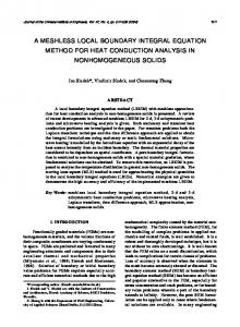
In contrast to temporal fixed stenoses, myocardial bridges are normal variants characterised by the compression of the coronary arteries due to myocardial muscle fibres overlying a segment of the artery. Myocardial bridges are most commonly found in the mid LAD, 1 mm to 10 mm below the surface of the myocardium with typical length of 10 mm to 30 mm. An angiogram of a myocardial bridge is shown in figure 2.5 (A). The major characteristics of myocardial bridges are: a phasic systolic vessel compression with a persistent diastolic diameter reduction, increased blood flow velocities, retrograde flow, and a reduced flow reserve [31]. Within the bridged segments permanent diameter reductions of 22 − 58 % were found during diastole, while in systole the diameters were reduced by 70 − 95 % [31]. A schematic drawing of the vessel compression and the mean pressure tracings within the bridge are given in figure 2.5 (B) and (C) respectively. The underlying mechanisms are fourfold. Firstly the discontinuity causes wave reflections, secondly the dynamic reduction of the vessel diameter produces secondary flow and thirdly there is evidence for flow separation in post stenotic regions [11, 15, 13]. Finally at severe deformations the artery may temporally collapse.

18


Figure 2.5: (A) Coronary angiogram of a myocardial bridge in the left anterior descending (LAD) branch in end systole. Compression of the artery during the heart’s contraction phase, i.e. systole, is a characteristic finding in myocardial bridging (see text for details). (B) Semi-schematic drawing illustrates end systolic lumen dimensions and (C) the measured pressure tracings proximal, within and distal the bridged segment. Picture taken from [31].

2.3. SIMPLIFICATIONS

2.3

19

Simplifications

Faced towards the overwhelming complexity of the human cardiovascular system we summarise the main simplifications made in one-dimensional blood flow simulations. In contrast to unsteadiness, several features of biological flows may be neglected in some situations. A list of common assumptions is given below: • blood is treated as incompressible Newtonian fluid • flow is assumed to be laminar • the heart is modelled by a volumetric inflow boundary condition • axial curvature of the vessels is neglected • arterial wall is assumed to be thin and incompressible • non-linear behaviour of the arterial wall is not considered • the effect of surrounding tissue and tethering is disregarded • the muscular activity of the blood vessels is neglected • only large arteries are accommodated in the network • branching angles in the vascular network are neglected • vessel geometry of the myocardial bridge is idealised • flexural rigidity of the vessel wall is neglected • deformation cross-section is simplified • the arteriolar and capillary circulation is comprised into a ”windkessel” boundary condition • chemical reactions and diffusion of materials are not considered • the auto-regulative feedback control is not considered • haemodynamic conditions are adjusted by parameter control

Although each is physiologically relevant, the analysis is greatly simplified when these can be evidentiary neglected, which is the case in most arterial flows. In spite of many simplifications made, the models are pre-eminently applicable to evaluate the dynamic behaviour of the blood flow in the cardiovascular system.

20

2.4


General fluid mechanical considerations

The mathematical description of the fluid mechanics involved in the circulation is challenging in many aspects, even under the above simplifications. However, one way to study this complex system is to consider flow in isolated segments with appropriate boundary and interface conditions. One can then hope that this description of vascular networks can explain the characteristic pulsatile shapes of pressure and flow in different locations.

2.4.1

Equations of motion

The equations of mass and momentum conservation fully describe the macroscopic behaviour of viscous flows. The equation of continuity states that the rate of mass accumulation is always equal to the difference between the rate of incoming and outgoing masses Dρ (2.4) + ρ (∇.~v ) = 0, Dt which for incompressible fluids simplifies to ∇.~v = 0.

(2.5)

The conservation of momentum follows from Newton’s second principle: Mass per unit volume times acceleration is equal to the sum of three volume forces: the pressure force, the viscous force and the external force D ~v ~ ~ − ∇.Γ ~ + ρ G. = −∇p (2.6) ρ Dt In these equations, D/Dt is the substantial derivative, ~v is the velocity vector of ~ is the external force. the flow field, p is the pressure, Γ is the stress tensor and G Assigning boundary conditions to the equations of motion yields a simplified set of equations, which is suitable for a specific type of flow problems. For example, the assumption of constant density and viscosity leads to the Navier-Stokes equations for incompressible Newtonian fluids D ~v 1~ ~ 2 ~v + G, ~ = − ∇p (2.7) +ν∇ Dt ρ ~ = 0, this reduces to the Euler equation and for negligible viscous effects, ∇.Γ D ~v 1~ ~ = − ∇p + G. Dt ρ

(2.8)

~ = 0. In this study we further assume that the external body force is zero, i.e. G The equations presented here are the fundamental equations used to derive the onedimensional model in chapter 3. In the following we briefly discuss the pressure and flow variables and their orders of magnitude.

2.4. GENERAL FLUID MECHANICAL CONSIDERATIONS

2.4.2

21

Pressure

In cardiovascular medicine the denotation of pressure is ambiguous. There is the transmural pressure, ptm , which is the pressure difference between the inside (pint ) and the outside (pext ) of a structure (ventricle, auricle or blood vessel) and the perfusion pressure, pperf , which is the difference in transmural pressure between two different sites (ptm1 , ptm2 ) in the vascular network. Perfusion pressure is also called the driving pressure. Mean aortic pressure minus mean venous pressure yields the mean perfusion pressure, which is responsible for the blood flow through the systemic circulation from the aorta to the vena cava. ptm = pint − pext

(2.9)

pperf = ptm1 − ptm2

(2.10)

20

Aorta

Left Ventricle

Left Atrium

Pulmonary Veins

Pulmonary Capillaries

Right Ventricle

Right Atrium

Vena Cavae

Large Veins

Small Veins

Venules

Arterioles

40

Small Arteries

60

Large Arteries

80

Capillaries

100

Aorta

Pressure [mmHg]

120

Pulmonary Arteries

The blood pressure is generally measured in mm of mercury (mmHg) 5 . Healthy young adults should have a systolic ventricular peak pressure of 16 kP a (120 mmHg), and a diastolic pressure of 10 kP a (80 mmHg). The pressure distribution in the vasculature is shown in figure 2.6.

0

Figure 2.6: Pressure distribution in the human vascular system redrawn from [14].

2.4.3

Flow rate

As well as the pressure the flow rate, q, is patient specific. However, the aortic pressure and flow waveforms under certain conditions are known from in vivo measurements. In our simulations, the flow rate is a synthetic waveform represented as 5

In Si-units 1 T orr ≡ 1 mmHg ≡ 133 P a.

22


exponential pulse wave with parameters for the amplitude and raising time. Frequently, we also use a synthetic oscillatory waveform of a measured pulse wave to reproduce experimental data. In each case the shape of the flow rate will be shown together with simulation results produced by it.

2.4.4

Dimensionless parameters

In order to simulate pulsatile flow in a model represented by segments of the cardiovascular system, a variety of similarity parameters characterise the flow behaviour in certain conditions. To investigate the importance of the pressure, viscous and transient forces, the following dimensionless numbers are defined: • The Reynolds number indicates the relative importance of the viscous forces compared to the inertial forces. It is defined as Re =

V` , ν

where ` is a characteristic length (such as the tube diameter), ν is the kinematic viscosity defined as ν = µ/ρ and V is the axial flow velocity 6 . Large Reynolds numbers indicate the dominance of convective inertia forces, while at low Reynolds numbers a strong influence of shear forces is observed. As already mentioned in the introduction the Reynolds number is a measure of turbulence. In circular tubes, three regions are recognised: laminar flow (0 < Re < 2300), transient flow (2300 < Re < 4000) and turbulent flow (Re > 4000). Since the geometry in the circulation is not √ regular, the characteristic length scale of the flow may also be defined as ` = A, where A is the cross-section of the vessel. Under resting conditions the typical Reynolds numbers in the circulation are: Re√A = 3800 in the ascending aorta, Re√A = 2800 in the abdominal aorta, Re√A = 450 in the coronary arteries, and can be as small as ten in small arteries. We note that, due to the complex geometry of the arterial system instabilities like flow mixing, vortex formation, reverse flow and turbulent behaviour may occur even at low Reynolds numbers. • The Womersley number is the ratio of the unsteady inertial forces to the shear forces. It is defined as r ω Wo = ` , ν where ω is the angular frequency, which for a harmonic oscillation with period T and frequency f = 1/T is defined as ω = 2πf . When the Womersley number 6

The Reynolds number may be also defined in terms of the average flow velocity.

2.4. GENERAL FLUID MECHANICAL CONSIDERATIONS

23

is small, viscous forces dominate, and as a consequence the velocity profiles are parabolic in shape [3, 4, 5]. At larger Womersley numbers the unsteady inertial forces dominate, and the flow shows relative flat velocity profiles. Typical values under resting conditions are W o√A = 33 in the abdominal aorta and W o√A = 4 in the coronary artery. As a consequence of increasing heart rate, the Womersley number increases under exercise. • The Strouhal number represents a measure of the ratio of unsteady inertial forces to the inertial forces which follow from changes in velocity from one point to another in the flow field. The definition is Sr =

ω` , V

which can be rewritten as Sr = W o2 /Re. It therefore combines the Reynolds and Womersley numbers. The Strouhal number is important for analysing unsteady, oscillating flow problems with moving walls. For small Strouhal numbers the influence of local acceleration on the flow is negligible so that the flow field can be assumed to be quasi-stationary, large values however require to specify the flow field in a temporal sense. Typical values in the circulation are Sr = 0.15 in the abdominal aorta and Sr = 0.08 in the coronary artery. • The speed index is analogous to the Mach or Froude number. It is defined as the ratio of local flow velocity to local wave speed S=

V , c

where c is the local wave speed. It determines the transition point from subcritical to supercritical flows. If the speed index S is less than 1 the flow is subcritical, a value of S > 1 indicates a supercritical flow.

There are numerous dimensionless parameters that are useful in fluid mechanics, however in this study we are concerned with the above mentioned.

24


Chapter 3 Averaged flow model

A

variety of blood flow models are based on the Navier-Stokes equation or emanate from simplifying assumptions. The following chapter starts with the axisymmetric Navier-Stokes equation for incompressible fluids and discusses the orders of magnitude for several terms in a non-dimensional manner. By asymptotic reduction and subsequent integration over the cross-section the system of non-linear equations is expressed in averaged flow variables (A, u, p). These equations are commonly accepted in quasi-one-dimensional models of the cardiovascular system [22, 23, 47, 18, 59, 118]. Essentially these models are based on five types of elements, namely, (i) quasi-onedimensional conduits, with lateral dimensions smaller than their length, (ii) locally restricted bifurcations, (iii) pathological segments (stenoses, aneurisms, stents, curved vessels), (iv) vascular termination (windkessel) and (v) aortic inflow condition. The main advantage of the quasi-one-dimensional formulation is that all important parameters can be identified by modern non-invasive measurement techniques, which is not the case for full three-dimensional models. The one-dimensional formulation, however, cannot resolve local blood flow patterns, e.g. flow and pressure distributions around stenoses or bifurcations, wall shear distributions, pressure drop or flow separation. As mentioned in chapter 2 the flow in the left main coronary artery is of entrance type and the vessel deformation in myocardial bridges is a spatiotemporal event. Constitutive relation between the pressure and cross-sectional area in time varying non-circular ducts needs to be derived in order to calculate the flows under these conditions. The assumption of large Reynolds number flow allows the approximate solution to this type of flow via a boundary layer formulation. For this purpose the flow is divided into two regions, one close to the walls, where the flow is viscous (boundary layer) and the other in the centre where the flow is mainly inviscid (core flow). We subsequently derive the boundary layer equations for axially symmetric flows and the Falkner-Skan similarity solution in a vessel with spatiotemporal dependent pressure gradient. The evolution of the boundary layer is assumed to be

25

26

CHAPTER 3. AVERAGED FLOW MODEL

quasi-stationary and the flow field is approximated by Hartree velocity profiles. Reasonable relations for viscous friction and momentum correction in the averaged flow equations are obtained from the von Kármán integral momentum equation. The chapter finishes with physiological conditions under which the considered model can give reasonable results.

3.1

Averaged flow equations

The following derivation is motivated by [48] , [49] and [50]. We consider the incompressible Navier-Stokes equations (2.7) in cylindrical coordinates (x, r, θ) with velocity components ~v (x, t) = (vx (x, t, θ), vr (x, t, θ), vθ (x, t, θ))T . We assume that all quantities are independent of the angular variable θ, so that the equations reduce to 2 ∂vx ∂ vx 1 ∂vx ∂ 2 vx ∂vx ∂vx 1 ∂p + vx + vr + =ν + + , (3.1a) ∂t ∂x ∂r ρ ∂x ∂r2 r ∂r ∂x2 2 ∂vr ∂vr 1 ∂p ∂ vr 1 ∂vr vr ∂ 2 vr ∂vr + . (3.1b) + vx + vr + =ν − 2+ ∂t ∂x ∂r ρ ∂x ∂r2 r ∂r r ∂x2 The continuity equation in cylindrical coordinates is given by ∂vx 1 ∂ + (rvr ) = 0. (3.2) ∂x r ∂r In flexible tubes the maximum value of the radial velocity, vr , is that of the wall, which is generally much smaller than the axial flow velocity, vx . The flow in the cardiovascular system is therefore essentially one-dimensional with its main flow direction along the axis of the tube. We define the dimensionless parameter E := and the dimensionless variables r x vx r∗ := , x∗ := , vx∗ := , R X Vx

Vr . Vx

vr∗ :=

vr , Vr

(3.3)

p∗ :=

p , ρ Vx2

t∗ :=

Vx t. X

(3.4)

For flow in large arteries like the aorta, carotid, or radial arteries the characteristic variables are typically Vx ≈ 0.5

m , s

Vr ≈ 5 ∗ 10−4

m , s

R ≈ 10−3 m,

ν ≈ 4 ∗ 10−6

m2 , s

(3.5)

so that the parameter E is of the order O(10−2 ). From the continuity equation (3.2) it follows that R Vx = X Vr , thus X = R/E ≈ 0.1 m. Insertion of the dimensionless variables (3.4) into the continuity equation (3.2) yields ∂ ∗ ∗ ∂ (r vx ) + ∗ (r∗ vr∗ ) = 0. ∗ ∂x ∂r

(3.6)

3.1. AVERAGED FLOW EQUATIONS

27

Expressing the first momentum equation (3.1a) in non-dimensional variables leads to 2 ∗ ∗ ∗ ∂vx∗ ∂p∗ 1 1 ∂ vx 1 1 ∂vx∗ ∂ 2 vx∗ ∗ ∂vx ∗ ∂vx + vx ∗ + vr ∗ + ∗ = + + E ∗2 , (3.7) ∂t∗ ∂x ∂r ∂x Re∗ E ∂r∗2 E r∗ ∂r∗ ∂x where Re∗ is the Reynolds number defined by Re∗ :=

Vx R , ν

(3.8)

which for typical characteristic variables is of the order O(102 ). The preceding factors on the right hand side of equation (3.7) favour the negligence of the last term involving E compared with E1 . Employing the continuity equation we obtain the first momentum equation in non-dimensional form ∗ ∂ ∗ ∗ ∗ ∂ ∗ ∗ 1 ∂ ∂ ∗ ∗ ∗ ∂vx (r vx ) + ∗ (r vx vr ) + ∗ (r p ) = r . (3.9) ∂t∗ ∂r ∂x E Re∗ ∂r∗ ∂r∗ Inserting the non-dimensional variables into the second momentum equation (3.1b) gives ∗ ∗ ∗ 2 ∗ ∂p∗ E ∂ 2 vr∗ 1 ∂vr vr 2 ∂vr ∗ ∂vr ∗ ∂vr 2 ∂ vr + vx ∗ + vr ∗ + ∗ = + − +E E (3.10) ∂t∗ ∂x ∂r ∂r Re∗ ∂r∗2 r∗ ∂r∗ r∗2 ∂x∗2 All terms except the pressure derivative on the left hand side of the above equation have a leading term of order O(10−4 ), so that in a first approximation the pressure does not change in radial direction, ∂p∗ = 0. ∂r∗

(3.11)

In the following the dimensionless continuity and momentum equation are integrated over the cross-section from r∗ = 0 to r∗ = R∗ . The integration of equation (3.6) leads to Z R∗ ∗ ∂ ∗ ∗ ∗ ∗ ∗ ∗ ∗ ∂r vx r dr − vx r + vr r = 0, (3.12) ∂x∗ 0 ∂x∗ r∗ =R∗ r∗ =R∗ and by the definition of the dimensionless mean flow in axial direction Z R∗ ∗ q := 2π vx∗ r∗ dr∗ ,

(3.13)

0

the continuity equation turns into ∗ 1 ∂q ∗ ∗ ∂R ∗ ∗ vx + R vr∗ = 0. −R ∗ ∗ 2π ∂x ∂x r∗ =R∗ r∗ =R∗

(3.14)

28


The integration of the first momentum equation (3.7) results in Z R∗ Z R∗ ∂R∗ ∗ ∗ ∂R∗ ∗2 ∗ ∂ ∂ ∗ ∗ ∗ ∗2 ∗ ∗ vx r dr − ∗ vx r vx r dr − + ∗ v r (3.15) ∂t∗ 0 ∂t ∂x 0 ∂x∗ x r∗ =R∗ r∗ =R∗ Z ∗ ∗ 1 ∂p∗ R ∗ ∗ ∂ ∗ ∗ ∗ ∗ ∂vx r dr = + vx vr r + ∗ r . ∂x 0 E Re∗ ∂r∗ ∂r∗ r∗ =R∗ r∗ =R∗ The kinematic boundary condition and the non-slip condition at the arterial wall state that the radial fluid velocity at the wall is tangential to the surface ∗ ∗ ∂r ∗ ∗ ∂r = vr + vx ∗ , (3.16) ∂t∗ r∗ =R∗ ∂x r∗ =R∗ r∗ =R∗ and that the axial fluid velocity, vx , at the wall is zero vx∗ = 0.

(3.17)

r∗ =R∗

Applied to the continuity equation this leads to ∂R∗ ∂q ∗ + ∗ = 0. ∂t∗ ∂x By defining another dimensionless parameter Z ∗ 2π 2 R∗2 R ∗ ∗2 ∗ ∗ r vx dr , χ := q ∗2 0 2πR∗

(3.18)

(3.19)

and using equation (3.16) and (3.17), the momentum equation (3.15) may be written as ∗2 ∗ ∗ ∂ 1 ∂ ∂q ∗ ∗ q ∗ ∂p ∗ ∂vx + ∗ χ ∗ +A = r . (3.20) ∂t∗ ∂x A ∂x∗ E Re∗ ∂r∗ ∂r∗ r∗ =R∗ The coefficient χ∗ is the ratio of momentum flux through a cross-section A∗ and the momentum flux with the average velocity through the same cross-section. It is constant if the velocity profile does not depend on x and is equal to one if vx∗ is independent of r (uniform velocity profile). The most general form of the cross-section averaged equations finally is ∂A∗ ∂q ∗ + ∗ = 0, ∂t∗ ∂x ∗2 ∗ ∗ q ∂q ∗ ∂ 1 ∂ ∗ ∗ ∂p ∗ ∂vx + ∗ χ ∗ +A = r . ∂t∗ ∂x A ∂x∗ E Re∗ ∂r∗ ∂r∗ r∗ =R∗

(3.21a) (3.21b)

These equations may be rewritten in terms of dimensional quantities through the definition of a dimensional volume flow Z R q := 2π vx r dr, (3.22) 0

3.1. AVERAGED FLOW EQUATIONS

29

which by definition leads to the expression q∗ =

q . Vx R

(3.23)

Finally the dimensional form of the one-dimensional equations for blood flow in arteries are ∂A ∂q + = 0, ∂x 2 ∂t ∂q ∂ q A ∂p + χ + = Fν , ∂t ∂x A ρ0 ∂x where the momentum correction, χ, is defined as Z R 2π v 2 r dr, χ := Au2 0 x

(3.24a) (3.24b)

(3.25)

and the viscous friction term

∂vx Fν := 2πνR ∂r

.

(3.26)

r=R

We finally rearrange the equations written in area and flow rate in terms of area and area-averaged axial flow velocity so that ∂Au ∂Ad ∂A0 =− + , (3.27a) ∂t ∂x ∂t ∂u u (χ − 1) ∂A u ∂ χu 1 ∂p Fν =− +u + + . (3.27b) ∂t A ∂x ∂x ρ0 ∂x A We have assumed that the total cross-sectional area is given by the equilibrium crosssectional area Ad and the pressure induced perturbation A0 , so that A = Ad + A0 . The derivative of Ad with respect to time on the right hand-side of equation (3.27a) is a prescribed function depending on the contraction of the cardiac muscles overlying the segment of the artery and is responsible for secondary fluid motion. Throughout this study we mainly discuss flow in specific arterial networks, so that the dimensional form of the equations is used. Closer attention reveals that the two equations posses three unknowns (A, u, p). To find a unique solution a third equation relating the pressure and cross-sectional area is required. This constitutive equation is the subject of the next Section.

30

3.2


Fluid structure interaction

As previously discussed arterial walls possess complex elastic behaviour, if the fluid is driven by an oscillating pressure gradient. Negligence of material nonlinearities and viscoelasticity simplifies the description, but nonetheless the equations are geometrically nonlinear – the diameter of the vessel varies with the pulsating pressure. In large vessels, such as the aorta, the carotid or the radial arteries, a maximum change of 10 % in the vessel diameter is expected. This results in the same change in the Womersley and Reynolds numbers. Even though a linearisation about an equilibrium cross-section is possible under these conditions, the cyclic deformation of the arterial wall in myocardial bridges is geometrically nonlinear and we dismiss this simplifying assumption. This section starts from a simplified geometry found in most myocardial bridges [119] and subsequently derives an analytical expression for the relation between the pressure and area of a non-circular tube. Finally the elastic properties and the wall thickness of vessels are related to their diameter by experimental findings.

3.2.1

Geometrical model

Our first geometrical simplification for modelling blood flow in arteries is that the axial curvature of the tube is assumed to be small everywhere, so that the problem can be defined in one space dimension along the x-axis. According to this we have simplified the anatomy of the myocardial bridge as shown in figure 3.1. The two arrows in figure 3.1 denote the location of either circular (B − B) or oval (C − C) cross-section of the tube. Due to the fact that the wall thickness, h0 , is small compared to the bending radius Rd (h0 /Rd 1), we assume that the bending stress inside the wall is negligible. Consequently the cross-section of a circular tube (figure 3.2 (left)) under deformation in z-direction, is given by the composition of a rectangle with two semicircular ends of bending radius Rd as illustrated in figure 3.2 (right). This is consistent with the predominately eccentric deformation of bridged segments found in [119, 29]. We note that negligence of bending stress causes the tube to collapse significantly earlier, i.e. the assumption is only satisfied if ptm ≥ 0. The deformation distance between the squeezing muscles and the width of the flat portion are denoted by D (x) and B (x, t) respectively. The equilibrium condition of the cylindrical tube figure 3.2 (left) is denoted by the inner radius, R0 , the circumference U0 = 2 π R0 and the cross-section A0 = π R02 . However, the equilibrium cross-sectional area of the deformed tube is Ad (x, t) (see figure 3.2 (right)). RThe total cross-sectional area in the yz-plane of the tube is defined by A (x, t) = A da and the actual circumference is Up (x, t). Consequently the average velocity is given by R 1 u (x, t) = A S ~vx da and the volume flux across a given section therefore is q (x, t) = A u.

3.2. FLUID STRUCTURE INTERACTION A−A

Ω1

usn (t)

Ω2

31

Ω3

Ω4

Ω5

5

5

5

5

5

4

4

4

4

4

3

3

3

3

3

2

2

2

2

2

1

1

1

1

1

0

0

0

0

0

-1

-1 -2

0

1

2

3

xs1

-2

4

lt1

1

2

3

4

-2

xs2

-1

-1

-1

0

0

1

2

3

4

-2

xs3

0

1

2

3

-2

4

xs4

0

1

2

3

4

xs5 w− ← pout (t) w+ →

−

w ← pin (t) w+ →

d

0

xt1 B−B

xt2

xt3

xt4

x

C −C

Figure 3.1: Schematic anatomy of a double myocardial bridge. The control segments Ωn are equally spaced. Observation locations for haemodynamic properties are in the centre of each segment at xsn , transitions between the segments are at xtn . The transition length between the segments is denoted by tln . The graphs above each segment illustrate the differences in flow velocity usn . To illustrate the deformation we have indicated two cross-sections B − B and C − C in the circular and non-circular segments respectively (see figure 3.2). The pressure at the inlet and outlet are given by pin and pout respectively, the characteristics ω + and ω − are discussed in chapter 4.

As shown in the angiography 2.5 and figure 3.1 the coronary arteries in myocardial bridges are structured by several wall deformations. Their number, degree and extension may independently vary with time, so that the axial curvature of the arterial wall for each of the n = 1...N myocardial bridges in series is characterised by N functions. The deformation is specified by a parameter ζ, defined as ζ = Rd /R0 , which is chosen in the stenosis n to vary with time as 1 ζn (t) = (ζdiastole − ζsystole ) (gn (t) + 1) + ζsystole , (3.28) 2 where gn (t) are periodic functions in t depending on the contraction of the muscle fibres. ζsystole and ζdiastole are fixed geometrical parameters between 0 and 1, specifying the degree of systolic and diastolic deformation respectively. We note that in the centre of the deformation ζ(x = xs2 ) = ζ0 , i.e. the degree of deformation increases with decreasing ζ0 and consequently ζsystole < ζdiastole . To represent the time dependence of the deformation found in intra-vascular ultra-sound (IVUS) measurements [120], a synthetic deformation waveform gn (t) given by m=1..3 sine/cosine harmonics is used. 3 X 0.8 gn (t) = sin(m ω (t − 4tn ) + φm ) m m=1

(3.29)

Here 4tn is the delay for each deformation with respect to the cardiac cycle (see figure 3.3) and φm are the phases in radian, chosen to be φ1 = 3.5, φ2 = 1.5, and

32

CHAPTER 3. AVERAGED FLOW MODEL C −C

B−B A0 (x, t) R(x, t)

h0

0.5 A0 (x, t)

z D(x)

Rd (x)

Ad (x)

y

A0 (x) Up (x, t) B(x, t)

Figure 3.2: The deformation geometry of a linear elastic circular tube under negligence of bending stress inside the wall. Cross-section B − B (left) shows circular expansion under pressure and the cross-section C − C illustrates the geometry under external deformation independent of z (right). The equilibrium cross-sectional area Ad is shaded in light grey, while the perturbation area A0 is shaded in dark grey. The dashed lines indicate expansion under pressure.

φ3 = 3.9. The axial curvature of each deformation is approximated by two hyperbolic tangent functions, so that N X

x − xtn+1 x − xtn − tanh , Rd (x, t) = R0 ζn tanh ltn ltn+1 n=1

(3.30)

where x is the axial coordinate and xtn are the transition locations. Equation (3.30) smoothes the transition between the segmental domains Ωn by a transition length ltn . The actual state of deformation can also be expressed by the ratio, ε, based upon the half-axes of the non-circular duct. ε(x, t) =

3.2.2

1 2

Rd B + Rd

(3.31)

The pressure-area relationship for non-circular crosssections

Due to its complicated structure, it is difficult to provide a synthetic mathematical description for the mechanical behaviour of vessel walls. Here, we focus on the most relevant structural features and the simplest mathematical model for arterial tissues and we subsequently derive an algebraic pressure-area relationship for a vessel under external deformation. In this context we characterise the relative change in crosssectional area with respect to the pressure increment according to A = A (Rd , p). Initially we assume that the actual behaviour of the arterial tissue for small deformations does not depend on the strain rate, and that the deformation is symmetric

3.2. FLUID STRUCTURE INTERACTION

33 2 4t

2

R d [mm]

R0

EKG

0

T P QRS

time [s]

0

1

Figure 3.3: The variation of the bending radius Rd (xs2 , t) in the centre of the deformation is plotted with respect to the cardiac cycle, represented by an EKG trace. The deformation function (solid line) is shifted with respect to the cardiac cycle by 4t = 0 ± 100 ms (dashed lines) to illustrate differences caused by the transit time of a pressure wave.

about the xy−plane. Under prior assumptions that the arterial wall is homogeneous and isotropic the theory of linear elastic shells is applicable [121]. The equation for R0 , the radial wall displacement of a infinite cylidrical shell is 2 0 ∂2 ∂ R Eh0 Θ 2 + 2 R0 = Φ, (3.32) 2 ∂x ∂x R where Φ is the total force per unit area acting in the radial direction including the stresses induced by the fluid. Henceforth we assume that Φ is equal to the transmural pressure ptm . The flexural rigidity Θ in equation (3.32) is given by Θ=

Eh30 , 12(1 − σ 2 )

(3.33)

where σ is Poisson’s ratio. The assumption of material homogeneity and isotropy indicates that E = Eθ = Ex and σ = σθ = σx , whereas typical values for biological tissues are 0.6 M P a and 0.5 respectively. The first term in the shell equation describes the effect of transverse shear, the second one the membrane force along the tangent to the cross-section. It was experimentally shown that the longitudinal motion of the arterial wall is very small [11, 15]. This behaviour is partially due to strong vascular tethering and partially due to the circumferential orientation of smooth muscles, through which the coupling of circumferential and longitudinal strain is minimised. Further we note that a thin shell has

34


little resistance to bending and the shear forces are small compared with the extensional ones, so that we can provide an explicit relation between the pressure and the vessel cross-sectional area A = π(R+R0 )2 . We denote the perturbation about the equilibrium area Ad (Rd ) by A0 (Rd , p), and hence the relation for the total cross-sectional area becomes dependent on Rd and we may write A (Rd , p) = A0 (Rd , p) + Ad (Rd ). Under the above assumptions the shell-equation (3.32) is p = E

h0 h0 = ςh , Rd Rd

(3.34)

where ςh is the hoop stress and is the circumferential strain given by =

U − U0 2πRd + 2B − 2 π R0 Rd B = = + − 1. U0 2πR0 R0 πR0

(3.35)

However if the tube is tethered against longitudinal displacements ξ, which is generally the case in the vasculature, a cancelling strain equal and opposite to ∂ξ σpR =− ∂x Eh0

(3.36)

must be supplied by applying longitudinal forces to the tube wall. The resultant longitudinal stress is comparable with the circumferential stress and produces just as that does, strains in perpendicular directions. The stress in a tethered tube is therefore given by Rd E , = (3.37) ςt = p h0 1 − σ2 Equation (3.35) and (3.37) lead to an expression for the pressure dependence of the width 1 − σ 2 Rd Rd B (Rd , p) = π R0 p+1− . (3.38) E h0 R0 The total cross-sectional area is A (Rd , p) = π Rd2 + 2 B (Rd , p) Rd .

(3.39)

In the unperturbed state, the cross-section is Ad (Rd ) = Rd U0 − π Rd2 .

(3.40)

We can finally write the pressure induced perturbation as A0 (Rd , p) = Rd2 U0 p

1 − σ2 . E h0

(3.41)

Application of equation (3.34) and (3.39) leads to the pressure-area relation for p ≥ 0 p (Rd , A) =

E h0 (π Rd2 + A − Rd U0 ) . (1 − σ 2 ) U0 Rd2

(3.42)


35

It should be noted that under the assumption of linear elastic material with constant elastic modulus, equation (3.39) and (3.41) have the property that the area increases linearly with excess pressure. Real arteries, however, resist over-expansion by having an incremental elastic modulus E() that increases with increasing strain [16]. It should be further noted that the area perturbation in equation (3.41) is not only dependent on pressure variation but also on the degree of deformation through Rd . This is due to the fact that the distensibility of the tube depends in some way on the wall geometry and its elastic properties. For a given cross-sectional area A it is defined as 1 ∂A DA := (3.43) , A ∂p A which according to equation (3.39) is 2 Rd ∂B (ζ, p) U0 Rd2 (1 − σ 2 ) = . A ∂p A E h0

(3.44)

The distensibility DA is directly related to the wave speed by 1 cA (x, t) = q , 1 ρ0 κ + D A

(3.45)

DA =

As previously discussed κ = 0 for incompressible fluids. The ζ0 -dependence of the above relations is shown in figure 3.4. At negative transmural pressure, however, the original shape buckles due to bending of the vessel wall and eventually collapses. To account for the strongly nonlinear behaviour another vessel wall parameter can be introduced to determine the linear/non-linear nature of elastic response $/2 U − U0 . (3.46) = U0 Linear behaviour is obtained for $ = 2, while for $ > 2 or $ < 2 the response is non-linear, i.e. stiffening or flagging of the wall. Consequently the width becomes " # 2/$ 1 − σ 2 Rd Rd B (Rd , p) = π R0 +1− p (3.47) E h0 R0 and the pressure area relation is E h0 p (Rd , A) = 1 − σ 2 Rd

(π (Rd )2 + A − Rd U0 ) Rd U0

$/2 .

(3.48)

Finally the distensibility is 4 R d A0 DA = p $ A R0

1 − σ 2 Rd p E h0

2/$ .

(3.49)

36


(a)

Compliance, area, wave and flow velocity versus deformation c, u ˆm˜

Ad [mm2 ]

s

35

25

30 20

dp

h dAd i kP a mm2

600

25

15

20

c (ζ0 )

400

Ad (ζ0 )

Ad (0)

15

10

dp dAd

(ζ0 )

10 5

u (ζ0 )

5

0

0 1

0.8

0.6

z

ζ0

0.4

0.2

200

0

0

(b) y

Figure 3.4: (a) Dependence of compliance, area, wave and flow velocity on deformation ζ0 . The gradient dp/dAd = DA1 Ad is the compliance per unit length. (b) d

Schematic illustration of the different stages of deformation.

3.2.3

Elastic modulus and wall thickness as a function of tube radius

As the model depends on the elasticity of the wall, their thickness and the vessel radius, we need to find a functional relation to measurements of the volume compliance given in [122]. The volume compliance is approximately given by Cvol =

dV 3A0 LR0 ≈ , dp 2Eh0

(3.50)

where V is the volume of a given segment and A0 is the average cross-sectional area. Following suggestions in [18] a relation for elastic properties is obtained by an


37

exponential curve fit to above data so that Eh0 = k1 exp (k2 R0 ) + k3 , R0

(3.51)

with the constants k1 , k2 , and k3 . With data for Cvol from Westerhof [26] , Stergiopulos [122], and Segers [123] (shown in figure 3.5) we obtain k1 = 2.0 ∗ 106 N m−2 , k2 = −2.253 ∗ 103 m−1 , and k3 = 8.65 ∗ 104 N m−2 . Elastic wall properties in dependence on vessel radius 0.8 curve fit data

Eh0/R0 [MPa]

0.6

0.4

Eh0 R0

= k1 exp (k2 R0 ) + k3

0.2

0

0

2

4

6

8 R0 [mm]

10

12

14

Figure 3.5: Curve fit (solid line) with a function of the form (3.51) to data [122] (crosses) converted by equation (3.50), both plotted over the tube radius R0 .

A functional relationship for the wall thickness of small to medium sized arteries subject to the vessel radius can be found in [124], where h0 = a R0b .

(3.52)

The parameters for a = 3.87 and b = 0.63 were obtained by a logarithmic fit to data including vessel radii between 100 µm and 3000 µm. For larger arteries the ratio of wall thickness and radius remained remarkably constant so that h0 /R0 ≈ 0.16 [125].

38


Both relations are shown in figure 3.6. We note that the wall thickness, the diameter and the elastic modulus of the vessel are difficult to measure because they change with pressure and age and show significant variation in different persons. For example the elastic modulus of the thoracic aorta varies between 0.036 M P a and 0.409 M P a; the lowest values were found in young people ( λ− , i.e. the characteristics of the system are discriminative and have opposite directions, which is indicated by the ± signs. Under prior assumptions the system is strictly hyperbolic and the wave speed of the nonlinear system, cA = √ρ01DA , is always positive and generally much larger than the velocity of blood. The characteristic variables are found by the √ ∂w± ∂w± integration of ∂∂W = L(M), i.e. that ρ0 DA . The explicit = 1 and = ±A ∂u ∂A U relation for the characteristic variables is obtained by subsequent introduction of the wave speed, so that Z u Z A 1 ± √ w (x, t) = du ± dA= (4.7) ud Ad A ρ0 DA p √ ρ0 DAd − ρ0 DA u − ud ± 2 p =u − ud ± 2 (cA − cAd ), √ ρ0 DAd ρ0 DA where cAd is the wave speed of the linearised system. The equilibrium condition (ud , Ad ) suggests that ud = 0 when A = Ad . A system of linearised equations can be written by introduction of perturbation variables A0 and u0 . The distensibility for the equilibrium condition is DAd =

U0 Rd2 (1 − σ 2 ) 2 Rd ∂L (ζ, p) , = Ad ∂p Ad E h0

(4.8)

and the pressure-area relationship in equation (3.48) reduces to p (Rd , A0 ) =

E h0 A0 . (1 − σ 2 ) U0 Rd2

The linearised system can be written as " # 0 0 Ad A ∂Ud ∂Ud A 0 = , + Md (Ud ) = 0 + 1 0 0 u x f u t ∂t ∂x ρ0 DAd Ad

(4.9)

(4.10)

with the following eigenvalues and eigenvectors of Md (Ud )   " ∂w+ ∂w− # p p √ 1 ρ0 DA Ad ρ0 DAd −Ad ρ0 DAd ∂Ad ∂Ad . λd (Md ) =  √ 1 d  , Ld (Md ) = = ∂w + ∂w − − ρD 1 1 ∂u0 ∂u0 0

Ad

(4.11)

56

CHAPTER 4. THEORETICAL ASPECTS

The characteristic equations for the linearised equations are found to be identical to those of the non-linear equations, however, the characteristic curves, along which the characteristic equations apply, are different. Z A 1 A0 A0 ± 0 p w (x, t) = u ± dA = u0 ± p = u0 ± cAd . (4.12) Ad ρ0 DAd Ad ρ0 DAd Ad Ad Here cAd = √ρ

1 0 DAd Ad

is the wave speed for the linearised system. Linearisation of the

equations therefore neglects the fluid velocity in the expression of the characteristic lines. Both systems are hyperbolic and subcritical, so that we require one boundary condition at each end of the tube. They are implemented through the characteristic system and use the following compatibility relations A0 =

Ad (w+ − w− ) , cAd 2

u0 =

(w+ + w− ) 2

(4.13)

for the linear system as initial guess to solve the nonlinear in- and outflow conditions.

4.3

Interface and boundary conditions

As mentioned earlier the human cardiovascular system is a closed system of tubular entities. Parameters and exact course of the major 175 arteries are found in table A.1 and figure A.1 in the appendix. The description as separate segments requires interface conditions at the bifurcations and physiological boundary conditions at places where the computational domain is terminated, i.e. in- and outflow conditions. These conditions are based on physical laws and physiological factors respectively. The implementation is based on the characteristic system. In the following section we will shortly discuss common conditions used in cardiovascular system dynamics.

4.3.1

Approximation of boundary characteristics

Different types of in/outflow conditions for the characteristics may be applied. Non-reflecting boundary conditions are useful to approximate the characteristics at the boundary. They are frequently implemented by one-way wave equations, which for the forward and backward travelling characteristics are given in (4.14) and (4.15) respectively. ∂ 1 ∂ ∂ 1 ∂ + + + w (x = L, t+δt) = + + w+ (x = L−δx, t) (4.14) ∂x λ ∂t ∂x λ ∂t ∂ 1 ∂ ∂ 1 ∂ − + w (x = 0, t+δt) = + w− (x = 0+δx, t) (4.15) ∂x λ− ∂t ∂x λ− ∂t

4.3. INTERFACE AND BOUNDARY CONDITIONS

57

This, however, assumes that the primary wave direction is normal to the boundary and that none of the discriminative characteristics w+ (x = 0, t) = 0 w− (x = L, t) = 0

(no right travelling wave), (no lef t travelling wave),

(4.16) (4.17)

enter the domain. We note that wave reflections will occur as those conditions are not satisfied. The above equations are used to implement both the in/outflow and branching conditions. The method of characteristics is used to approximate the characteristic variables w+ and w− at the boundary at x = 0 and x = L. As illustrated in figure 4.1, w+ characteristics leave the domain at x = L, while w− characteristics leave the domain at x = 0 as time increases. t

w−

w+

w−

w+ x

x=0

x=L

Figure 4.1: Plane of independent variables. Approximation of boundary characteristics by one-way wave equations. As time increases positive characteristics w+ leave the domain at x = L, while negative characteristics w− leave the domain at x = 0.

4.3.2

Inflow boundary conditions

The inflow boundary condition at the aorta is given by the flow velocity, the area, or a relation between them. The shape of the pulse wave in the ascending aorta is mainly generated by the aortic valve. The pressure-flow conditions are known from in vivo measurements, so that either a periodic extension of a measured flow wave or a synthesised wave in the exponential form −t2 −t2 t 2t 2 2 2 t t qin (t) = q0 exp r + exp r (4.18) tr tr is used. Here the amplitude of the exponential waveform is q0 , while tr is the rising time. For reasons that the coronary flow is primarily driven by the aortic pressure,

58


the pulsatile boundary condition to the left main coronary artery was represented by a periodic extension to a synthetic pressure wave in the exponential form pin (t) = ps + p0

−t2 t exp 2t2r , tr

(4.19)

where ps is the static pressure and p0 is the amplitude of the exponential waveform. The parameters used in the simulations are specified later in the text.

4.3.3

Interface conditions

The branching conditions for a bifurcation shown in figure 4.2 are physically motivated by the conservation of mass and the requirement of constant pressure at the branching point [23]. The subscripts p, d1 and d2 stand for the parent, 1st and 2nd daughter vessels respectively. The mass flux balance is qp = qd1 + qd2 , while the enptp = ptd1 = ptd2 qd1 qp qd2

Figure 4.2: Flow and pressure in a vascular bifurcation. The subscripts p, d1 and d2 stand for the parent, 1st and 2nd daughter vessels respectively. ergy conservation leads to continuity of total pressure pt , i.e. ptp = ptd1 = ptd2 . The interface conditions for the nonlinear system are therefore Ap up = Ad1 ud1 + Ad2 ud2 , 1 1 pp + ρ0 u2p = pd1 + ρ0 u2d1 , 2 2 1 1 pp + ρ0 u2p = pd2 + ρ0 u2d2 , 2 2

(4.20) (4.21) (4.22)

while the linear system has similar conditions except that the static pressure is continuous across the bifurcation [23].

4.3. INTERFACE AND BOUNDARY CONDITIONS

4.3.4

59

Outflow boundary conditions

There are several ways to account for peripheral reflections at the terminals starting from pure resistive load, where the outflow is proportional to the pressure over three and four-element windkessel models [14, 57] to a structured tree (fractal) outflow condition suggested in [59]. In the current simulations we have implemented a three-element windkessel model for the termination of the arterial network [25, 64]. The main advantage of this model is to consider the compliant-capacitive effects due to micro-vessels and arterioles. The lumped analogue electrical circuit is shown in w− ← w+ →

Rc Cp

Rp

ground Figure 4.3: Three-element windkessel analogue circuit. figure 4.3. According to [64] the differential equation in the time domain satisfied by the circuit is ∂q p q(Rp + Rc ) ∂p = Rc − + , (4.23) ∂t ∂t Rp Cp Rp Cp with Rp and Cp being the peripheral resistance and compliance respectively. However Rc is the characteristic impedance of the terminating vessel, which for large vessels is a real number and modelled by a resistor. The total peripheral resistance Rt = Rp + Rc for each of the terminals was estimated by the total arterial peripheral resistance and the distribution of flow through the various branches [122]. The ratio Rc /Rt was estimated in [134] by fit to data and found to be approximately 0.2. Finally, the arterial compliance Cp for each segment was estimated from the total volume compliance [26]. Parameter values for Rt and Cp found in [20, 122] are listed in table A.1 in the appendix.

60


Chapter 5 Numerical Aspects

S

everal numerical challenges must be overcome before an adequate solution to afore mentioned equations is obtained. Not only the complex dynamical behaviour and non-linearity of the system but also the difficulties in boundary and interface conditions of arterial networks have to be addressed. Due to the non-linear terms in equation (3.85) and (3.27b) the solutions for haemodynamically developing flows are generally more difficult to obtain than fully developed flows or oscillating flows with a frequency dependent Stokes boundary layer. Developing flows require simultaneous solution of the continuity equation (3.27a), the momentum equation (3.27b) and the integral momentum equation (3.85), together with the boundary conditions given in (4.18), (4.20 - 4.23) and (3.86). The momentum correction factor and the viscous friction in equation (3.27b) are given by the solution to the integral momentum equation (3.85) and the two curve fits to the Falkner-Skan equation in (3.94) and (3.95), i.e. through the solution of equation (3.102) and (3.103). A structogram of the algorithm can be found in figure 5.4 at the end of this chapter .

5.1

Choice of numerical method

A variety of numerical schemes were used in blood flow simulations. Besides finite difference and finite volumes schemes there is the branch of spectral methods and the method of characteristics. Finite difference schemes are constructed by replacing continuous derivatives with appropriate finite difference approximations defined by a set of discrete points. Further distinction is drawn between up/downwind and central differences. The oscillatory nature of (non-linear) hyperbolic equations is known to raise high frequency oscillations (with wavelength 2 dx), when centrally differenced, because the value of the slope estimated is independent of the value of the dependent variable at the mid-point. Those oscillations can be reduced by upwind methods, because disturbances in the flow regime that affect convective acceleration can not

61

62

CHAPTER 5. NUMERICAL ASPECTS

be propagated upstream. However they are generally only first-order accurate and in practical applications, the MacCormack scheme for the solution of the non-linear equations is recommended. Detailed comparison of finite difference schemes for nonlinear differential equations is presented in [102]. Higher order corrected schemes can be found in [103]. For simplicity we have chosen an explicit second-order MacCormack predictorcorrector method as the basic scheme to discretise the set of equations. The two-step algorithm contains a small amount of both numerical diffusion and dispersion, which makes it numerically stable. More importantly this scheme is non-linearly stable, and has been successfully used to solve similar equations [102]. Besides the ability to treat interface and boundary conditions of the arterial network the method is able to resolve regions where strong, sharp gradients exist. Throughout this chapter we use a regular grid with uniform temporal and spatial grid intervals. In this way consistency is automatically achieved, while stability is not guaranteed. The stability of linear hyperbolic equations discretised by explicit finite difference methods is generally given by the CF L condition (Courant, Friedrich, Levy, 1928). However, the averaged flow equations are non-linear, and a rigourous stability analysis for these equations is exceedingly difficult. Therefore, the CF L condition can only be considered as a general guideline here, and the maximum allowable time step (with respect to stability) for any particular problem will vary about the predicted value and is determined by numerical experimentation. All simulations where performed under those criterions and are found to be valid in the region of interest.

5.1.1

Discretisation of the averaged flow equations

Starting from the initial conditions at time level (n), the flow variables at the interior nodes are predicted from the initial boundary condition in equation (4.18) or (4.19) by a backward difference in space, while a forward difference in space of the predicted variables is used in the corrector step. The direction of both prediction and correction is alternated at each time step (wind averaging). The first prediction step was chosen in the direction of wave propagation, because the scheme produces better results. To calculate future values at (n + 1) the scheme requires values at (n). In the following discretisation the subscript i indicates the nodes along the axis of each segment, m, and the superscript n refers to the time level, i.e. the spatial grid in axial direction is given as 0 ≤ i ≤ I with step width dx, and the grid over time is 0 ≤ n ≤ N with step width dt. The variables u• , A• and p• are intermediate predicted values of u, A and p respectively. The corrector step provides the final value of u, A and p at time (n + 1). The discrete spatial operators for the predictor step for even time steps (n mod 2 = 0) can be written as dq dx

=

n qi+1 − qin , dx

5.1. CHOICE OF NUMERICAL METHOD

63

pn − pni dp = i+1 , dx dx (χ u)ni+1 − (χ u)ni d(χ u) = , dx dx while for odd time steps (n mod 2 6= 0) they are n q n − qi−1 dq = i , dx dx pn − pni−1 dp = i , dx dx (χ u)ni − (χ u)ni−1 d(χ u) = . dx dx

Discretisation of mass and momentum conservation with an Euler step yields dq (A0 )•i = (A0 )ni − dt − (Ad )n+1 − (Ad )ni , i dx n u(χ − 1) n dq d(χ u) 1 dp Fν n • . ui = ui − dt +u + − A dx dx ρ dx A i 0 i

(5.1) (5.2)

The discretised spatial derivatives of the corrector step for even time steps (n mod 2 = 0) are given by (q • )ni − (q • )ni−1 dq • = , dx dx (p• )ni − (p• )ni−1 dp• = , dx dx (χ u• )ni − (χ u• )ni−1 d(χ u• ) = , dx dx while for odd time steps (n mod 2 6= 0) they are (q • )ni+1 − (q • )ni dq • = , dx dx (p• )ni+1 − (p• )ni dp• = , dx dx (χ u• )ni+1 − (χ u• )ni d(χ u• ) = . dx dx Discretisation of mass and momentum conservation in the corrector step of the MacCormack scheme is accoring to [102] (A0 )n+1 i un+1 i

1 dq • 0 0• n = (A + A )i − dt − (Ad )n+1 − (Ad )ni , (5.3) i 2 dx • n • u (χ − 1) n dq • 1 dp• Fν 1 • n • d(χ u ) = (u + u )i − dt +u + − .(5.4) • 2 A dx ρ0 dx A• i i dx

64


Care must be taken while discretising squared variables, as they appear in conservative form (i.e. as in equation (3.24a) and (3.24b)), because the finite difference equation in conservative form loses information about the sign of the velocity. This is called weak numerical instability. The difficulty is solved by replacing (q 2 )ni+1 − (q 2 )ni by n n n n 0.5(qi+1 + qin )(qi+1 − qin ) and (q 2 )ni − (q 2 )ni−1 by 0.5(qin + qi−1 )(qin − qi−1 ) [102]. predictor

corrector

n mod 2 6= 0

n mod 2 = 0

n+1

n+1

n i-1

i

i+1

n i-1

i

i+1

n mod 2 6= 0

n mod 2 = 0 n+1

n+1

n

n i-1

i

i+1

i-1

i

i+1

Figure 5.1: Stencils for the wind averaging MacCormack scheme. Predictor and corrector stencils are given for even (n mod 2 = 0) and odd time steps (n mod 2 6= 0). Desired values at n + 1 are illustrated as ~, required values for the computation are illustrated as . We note that the averaged flow conditions are solved for all vessels in the network, before the boundary layer properties are determined. This is possible, because the averaged flow equations are only dependent on prior values of momentum correction factor and the viscous friction.

5.1.2

Discretisation of the von K´ arm´ an momentum equation

The integral boundary layer equation (3.85) is discretised by a first order upwind scheme, the resulting discrete equations are iteratively solved for δ ∗ . The spatial derivatives are δ∗ n n − θi−1 dθ H i = , dx dx

5.1. CHOICE OF NUMERICAL METHOD

65

n V n − Vi−1 dV = i , dx dx (rj )n − (rwj )ni−1 drwj = w i . dx dx

The discretisation of the stationary and transient integral momentum equation is j dθ 2 δ∗ drw ∗2 V + δ + 1+ f1 − vw − H ∗ f2 , 0= δ (5.5) j ν i dx H ν νHrw i i dx # " n j v n ∗ n dV ∗ )n 2 )n dθ c 2θ + δ θ dr (V δ (V w f w i + + − − dt.(5.6) (δ ∗ )n+1 = − n+1i i j dx V V 2 i Vin+1 Vi rw i dx i dx

∗V

We note that the closure relations in equation (3.94) and (3.95) restrict the rage 1 δ ∗2 ∂V of validity, firstly because 2.4 > −1 has to be satisfied in the former relation ν ∂x and secondly due to the singularity at H = 1, 0 in the latter relation. The interval of solutions for δ ∗ therefore is restricted to the range 2 < H < 20, where the curve fits to the Falkner-Skan equation provide good approximations. Because the NewtonRaphson iteration is inappropriate for this type of problem the solution is obtained by a combined root bracketing, interval bisection and inverse quadratic interpolation method of van Wijngaarden-Brent-Dekker. Detailed description of the method can be found in [135]. The confining upper and lower brackets of δ ∗ required by the algorithm are set by solving equation (3.94) with an adaptive forward and backward iteration until either H ≈ 2 and H ≈ 20 or the above restriction is reached. Blasius

F alkner − Skan

δ∗

i=0 i=3

x

Figure 5.2: The boundary condition in equation (3.86) is prescribed a few grid points downstream (at i = 3) by computing the Blasuis solution for i ≤ 3. Downstream marching of equation (3.85) leads to values of δ ∗ at grid points i > 3. The thick solid line indicates the curvature of the vessel wall, while the boundary layer is illustrated by a dotted line.

66


The entrance boundary condition in (3.86) is satisfied by the Blasius solution, which was shown to be the leading order term [80]. The computation is started a few grid points downstream from the inlet, where the Blasius solution provides values of the boundary layer thickness at each time step (see figure 5.2). We note that the vessel has to be uniform at the transition location Blasius/Falkner-Skan. The solution was applied to the steady integral momentum equation as boundary condition for δ ∗ . Downstream marching the solution by the above method leads to the values of boundary properties along the tube axis. Through equation (3.102) and (3.103) one obtains the required values for momentum correction and viscous friction in the averaged flow equations (3.27a) and (3.27b).

5.2

Numerical treatment of boundary conditions

To implement the boundary and interface conditions it is convenient to neglect viscous friction. As described in the previous chapter the implementation of boundary conditions at each vessel in- and outlet comprises the approximation of boundary characteristics together with the application of compatibility relations. Non-reflecting or open boundary conditions are implemented by using inward differences for discretisation of equation (4.14) and (4.15). By this method the outgoing characteristics do not notice the boundary at all, i.e. they leave the domain into an infinitely long tube with constant impedance. We note that great care needs to be taken with the boundary conditions to ensure that spurious solution modes do not lead to numerical instabilities. Therefore the upwind boundary is treated by upwind biased method, because the general non conservative second-order upwind scheme produces instability for explicit time differencing [136]. (w− )n+1 = (w− )n0 + (w− )n1 − (w− )n−1 − 0 1 dt − n λ− (w )1 − (w− )n0 − (w− )n−1 + (w− )n−1 , 2 1 dx (w+ )n+1 = (w+ )nI + (w+ )nI−1 − (w+ )n−1 I I−1 − dt + n−1 λ+ (w+ )nI − (w+ )nI−1 − (w+ )n−1 I−1 + (w )I−2 . dx

(5.7)

(5.8)

The flow variables at the boundaries and the characteristics that enter the domain are obtained by the application of a specific boundary condition (in-/outflow or interface condition) and the compatibility relations in equation (4.13). Non-reflecting boundary conditions therefore simply assume that (w− )ni=I = 0, i.e. no left travelling characteristic w− enters the right end of the tube. Other boundary conditions are easily implemented for different applications.

5.2. NUMERICAL TREATMENT OF BOUNDARY CONDITIONS w−

67

w+

n+1

n

n-1 i=0

i=1

i=2

i=3

i = I-3

i = I-2

i = I-1

i=I

Figure 5.3: Stencils for the for the approximation of boundary characteristics. Desired values at n+1 are illustrated as ~, required values for the computation are illustrated as .

5.2.1

Inflow condition

At the inlet boundary x = 0 the variation of A and u is known by equation (4.18) or (4.19), so that together with the compatibility relations in equation (4.13) the entrance characteristic w+ is easily determined. However the non-linear system requires subsequent Newton iteration for solution, because the boundary condition is non-linear.

5.2.2

Bifurcations

On the basis of above approximation the characteristics which enter the arterial − − are known quantities. The reflected and transmitted bifurcation, wp+ , wd1 and wd2 characteristics in each segment are obtained by the solution of the interface conditions in equation (4.20) - (4.22). Starting point for the solution to this non-linear boundary value problem is given by analytic solution to the linearised conditions. Subsequent Newton iteration gives the final results for A and u in parent and daughter vessels, which through equation (4.8) and (3.43) directly lead to the required characteristics in participating segments.

5.2.3

Outflow condition

The discretisation of the windkessel outflow boundary condition is taken into account by solution to equation (4.23). As before the boundary characteristics which leave the domain are known quantities, so that compatible characteristics which enter the domain are found by discretisation of equation (4.23) and iterative solution for A and u.

68


read simulation parameters and initialise computational grid for n (1) N while ∆ u < 10 -6 Solve inflow condition eqn. (4.18) or (4.19) compatibility conditions eqn. (4.13) for m (1) M for i (1) I predictor step eqn. (5.1) and (5.2) boundary characteristics eqn. (5.7) and (5.8) for m (1) M for i (1) I corrector step eqn. (5.3) and (5.4) boundary characteristics eqn. (5.7) and (5.8) for m (1) M while ∆ δ < 10-6 von Karmann integral eqn. (5.5) and (5.6) Curve fit to Falkner-Skan eqn. (3.94) and (3.95) displacement area eqn. (3.99) and (3.100) momentum correction coefficient eqn. (3.102) viscous friction term eqn. (3.103) for m (1) M satisfy boundary conditions: boundary characteristics eqn. (5.7) and (5.8) while ∆ p < 10-6 interface conditions eqns. (4.20) - (4.22) windkessel outflow condition eqn. (4.23) write simulation data to harddisc and generate simulation report N M I

: number of time steps : number of segments in the network : number of grid points in a segment

Figure 5.4: Structogram for the boundary layer algorithm.

Chapter 6 Simulation Results

B

ased on the arguments raised in the previous chapters, this chapter presents the simulation results of steady and unsteady flow in a model of the human vascular system as a typical haemodynamic application. The proposed boundary layer method to model viscous friction and momentum correction in the entrance region of a tube with varying cross-section was subsequently applied to a test geometry, which consists of a single elastic tube with either temporally fixed or dynamic indentations, and specific clinical situations of myocardial bridging in the LCA as described in [40]. The pressure drop characteristics, the mean fractional flow reserve and the wall shear stress are computed and results are compared to those available in the literature. The simulations were carried out in stenosis of different degree and extent. The Womersley and Strouhal number were around 4 and below 0.15 respectively, the Reynolds number in the stenosis varied from 850 to 1500. The wave velocity in those situations may take values as low as c = 5 m/s in uniform vessels, rising to values around c = 30 m/s in constricted vessels. Physiological peak flow velocities, V, are much smaller, generally around 0.5 − 1 m/s, but they can reach 2 − 3 m/s in parts of severe deformation. The spatial resolution of the grid was adjusted to represent the curvature of deformation, where 4 gird points per mm was reasonable in any of the cases, the time resolution was chosen accordingly and ranged between 5 µs and 10 µs. These resolutions are sufficient to avoid numerical instabilities at severe deformations. The computational time required, for the simulation of one pulsatile cycle in a network of coronary arteries, was about 22 min. on an Apple Power-Mac G5, 2 GHz. However simulations of the main 175 arteries require considerably more computational time (about 2 to 3 hours per pulsatile cycle). We note that at least three pulsatile cycles are required to obtain steady state conditions. Generally we found that under application of a uniform flow profile at the entrance the core velocity in the vessel increases gradually downstream, indicating the development of a parabolic flow profile. For a Reynolds number of 800 the distances over which the core velocity stabilised in the tube were very much shorter than at 69

70

CHAPTER 6. SIMULATION RESULTS

2000; fully in line with the dependence of the entrance length. However fully developed flow was not present in any of the cases. In the following we address the flow limiting effect by the assessment of the pressure derived fractional flow reserve in different stenotic environments (test geometry and LCA). Further, we will discuss the pressure drop ∆p, the flow separation, the wall shear stress and the influence of external wall deformation. In some of the graphs we have shown the interval of possible solutions that may occur during the pulsatile cycle, i.e. the upper and lower envelope denoted by M axenv (solid red line) and M inenv (solid blue line) respectively.

6.1

Modelling: test geometry

We have chosen the test geometry of the tube according to the size of the left main coronary artery with an internal diameter of 5 mm. To observe separation and reattachment we have adapted the length to the maximum extent of the recirculation zone, which was about 300 mm at 80% diameter deformation. At 20 mm downstream of the entrance, the diameter was abruptly decreased (tl = 4 mm) by 0−85%, with an extent of 30 mm (single stenosis), another constriction with the same length follows 30 mm further downstream (double stenosis). In addition the extent of the single stenosis (short) was varied by a factor of two (medium) and three (long), in the double stenosis we varied the separation distance between one and three dimensions of the stenosis. The region around the diameter transition in the test geometries is shown in detail in figure 6.1. The area perturbation A0 , shown on the top of each column, indicates that the arterial deformation caused by pulsatile pressure is much smaller in regions where the tube is squeezed (A0 /A = 1−2%), while in circular segments A0 /A = 8−9%. Due to incompressibility and mass conservation a sudden jump to a high velocity is seen at the narrowing. It appears that the stenosis influences the mean velocity only over a short distance upstream, while in the case of flow separation the core velocity slowly decays until reattachment, then it starts growing again until the flow is fully developed. The boundary layer separation in the post-stenotic region indicates an emerging top-hat velocity profile from the stenosis, with sideway counter-current flows. The decay in core flow velocity indicates shear widening of the top-hat until reattachment. Further downstream the core velocity is almost constant. It was found that the distance over which the outlet effect occurs is smaller for short stenosis with small deformation and small Reynolds number.

6.1. MODELLING: TEST GEOMETRY short (s)

71 long (l)

medium (m)

double (d)

u(x),V (x) [cm/s]

2

A'(x) [mm ]

3 2 1 0 250 200

V

150 100

u

50

Rest : 1412

Rest : 1088

Re st : 1112

Re st : 868

0

p(x) [kPa]

20 15 10 5

p1

p3

p3

0 0.1

p1 p3

p2

p3 Max env

0.08 cf (x)

p1

p1

Min env

0.06 0.04 0.02

∗ δ /R(x),χ (x)

WSS(x) [Pa]

0 60 40 20 0 5 4 3 2 1 0 10

H(x)

8 6

sep.

H0 = 2.59 reat.

4 2

Rd(x) [mm]

0

2.5 0 -2.5 0 0.06 0.12 0.18 0.24 0.3 0 0.06 0.12 0.18 0.24 0.3 0 0.06 0.12 0.18 0.24 0.3 0 0.06 0.12 0.18 0.24 0.3 Axial vessel position x [m] Axial vessel position x [m] Axial vessel position x [m] Axial vessel position x [m]

Figure 6.1: The area perturbation, flow velocity, pressure, friction coefficient, the wall shear stress, momentum correction factor, the normalised boundary layer thickness and the shape factor are plotted as a function of position in a vessel with fixed deformation of ζ0 = 0.2. Three stenoses of different extent (s), (m) and (l) and a series stenosis (d) are compared. To indicate the flow characteristics in the stenosis we have used the Reynolds number Rest inside the deformation.

72


u(x), V(x) [cm/s]

15

WSS(x) [Pa]

cf (x)

p(x) [kPa]

(a) 300 250 200 150 100 50 0 20

(b)

(c)

10 5 0 0.1 0.08 0.06 0.04 0.02 0

FFR : 0.71

FFR : 0.70

FFR : 0.68

Max env Min env

60 40 20 0

∗

δ /R0(x), χ (x)

4 3 2 1 0 8 H(x)

6 4 2

Rd (x) [mm]

0 2.5 0 -2.5 0

0.06 0.12 0.18 0.24 0.3 0 0.06 0.12 0.18 0.24 0.3 0 0.06 0.12 0.18 0.24 0.3 Axial vessel position x [m] Axial vessel position x [m] Axial vessel position x [m]

Figure 6.2: In columns (a), (b) and (c) we compare a series of two dynamic stenoses, which are separated by one, two and three stenosis dimensions respectively. From the top we illustrate the flow velocity, the pressure, the friction coefficient, the wall shear stress, the momentum correction coefficient and normalised boundary layer thickness, the shape factor and the actual geometry of the vessel. The boundary layer is illustrated as dashed lines. The FFR decreases with increasing distance between the stenoses.

6.1. MODELLING: TEST GEOMETRY

73

The core velocity influences the frictional losses and the extent of the separation zone in series stenoses, so that series stenoses cannot be represented by two similar building blocks. This becomes more evident through the fact that the entrance flow profile in the second stenosis changes, if the distance of the two stenoses is varied (see figure 6.2 (a – c)). In developing flow conditions the downstream deformation is generally dominant in wall shear stress and frictional forces as well as in the extent of the post-stenotic separation zone. Further, it is likely that a downstream stenosis with equal deformation collapses significantly earlier, because the core flow velocity is increased, so that the transition from subcritical flow (S < 1) to supercritical flow (S > 1) happens earlier. The following sections will discuss the major haemodynamic conditions in myocardial bridges with reference to figure 6.1 and 6.2 in further detail.

6.1.1

Pressure drop and flow limitation

Geometric influences on the pressure loss across series of stenoses have been studied in [74]. The authors found that the pressure drop across severe stenoses is little affected by the eccentricity of the stenosis, dominantly affected by the severity and length of the stenosis, and affected by the Reynolds number only at low Reynolds number. Further [65] found that the eccentricity of mild stenoses increases the likelihood of collapse of stenotic arteries, because the buckling pressure is reduced. As in [27, 34] we found that the pressure proximal to the deformation is increased if the degree of deformation or the length of deformation is increased (see figure 6.1). Compared to the mean reference pressure (no deformation) of 9.29 kP a, the mean pressure at the inlet for a deformation of ζ0 = 0.2 was 10.28 kP a, 11.53 kP a and 12.41 kP a in the cases (s), (m) and (l) respectively. Under these conditions the mean flow in the reference artery was 10.36 cm3 /s. For fixed deformation of ζ0 = 0.2 we found 8.43 cm3 /s, 6.38 cm3 /s, 4.94 cm3 /s and 6.66 cm3 /s in the short, medium, long and double stenosis respectively. The pressure drop for the medium sized stenosis was at 7.52 kP a just below that of the double environment with 7.78 kP a, the pressure drop across the short stenosis was 4.15 kP a and across the long stenosis 9.82 kP a. In double stenoses the pressure drop across the proximal stenosis was 3.28 kP a, which is markedly less than 4.4 kP a at the distal stenosis. Complementary the values for the dynamic case are generally less pronounced, they can be found in table 6.1. However, the translesional pressure drop in a series of two stenoses in the entrance region of a tube shows further remarkable effects. The simulations indicate that in general the pressure drop cannot be obtained by a summation of pressure drops for single stenosis, since the proximal and distal stenosis influence each other unless the spacing between them exceeds some critical distance, which depends on the Reynolds number and deformation. Therefore several consecutive stenoses along the same epicardial artery require separate determination of stenosis severity. We found that when two stenoses are close together, the pressure drop is approximately equal to that of a

74


Table 6.1: Mean flow quantities, pressure drop and fractional flow reserve for test geometry shown in figure 6.1 meas. p¯1 4p1−3 F F Rp q¯1 u¯1

unit kP a kP a % cm3 /s m/s

fixed (s) (m) (l) (d) 10.42 11.63 12.48 11.46 4.15 7.52 9.82 7.78 60 35 21 32 8.43 6.38 4.94 6.66 0.43 0.33 0.25 0.34

(s) 9.55 1.89 80 9.90 0.50

dynamic (m) (l) 9.84 10.07 2.74 3.47 72 65 9.40 9.01 0.48 0.46

ref (d) 9.80 2.87 70 9.46 0.48

9.29 1.23 86 10.36 0.53

stenosis with twice the length of a single stenosis (see table 6.1 and figure 6.1 (m) and (d)). This can be explained by the fact that the friction coefficient in the recirculation zone between the two stenoses is small and consequently the pressure loss over that region is small. However, when the stenoses are separated by more than the length of the stenosis the flow is hardly affected by the second stenosis, because the core flow velocity and likewise the frictional force are increased (see figure 6.2 (a – c)), even though the entrance flow conditions are preserved. Coexistent is the increased reduction in shape factor and momentum correction coefficient, suggesting the non-linear influence in that region. The pressure drop over the downstream deformation is generally pronounced, however the distance between the deformations further increases the pressure drop and consequently the mean FFR is reduced. The values for the cases (a) to (c) are 4pa = 3.45 kP a, 4pb = 3.64 kP a and 4pc = 3.89 kP a for the pressure drop over the downstream deformation and F F Ra = 71 %, F F Rb = 70 % and F F Rc = 68 % for the mean fractional flow reserve across the bridge. We note that these findings are based on the entrance type of flow, where the core flow velocity gradually changes and may not appear in fully developed flow, where the core flow velocity is a constant and identical to the maximum of Hagen-Poiseuille flow velocity.

6.1.2

Separation and reattachment

The core velocity in a uniform tube generally increases downstream of the entrance, however in presence of a stenosis the boundary layer thickness decreases at the inlet and rapidly increases in the diverging part of the constriction (see figure 6.1). Separation occurs under the development of a top hat profile with sideway counter-current flow. At the separation point (N) the boundary layer thickness increases and a sudden jump in χ is evident, because the integral of the actual velocity vx2 over the area of the recirculation is close to zero and in contrast to the mean flow velocity the core velocity is increased. Therefore the non-linear term is pronounced in the separation region, while it is close to unity in converging regions. We note that the momentum correction becomes markedly smaller than before the upstream stenosis. This indicates that the


75

entrance profile into the second stenosis is almost flat, but has increased core velocity, while the counter current flow at the wall has disappeared. The reattachment of the boundary layer (H) further downstream is caused by momentum diffusion from the inviscid core into the the recirculation zone and the friction between the shear layers. The widening of the central core reduces the flow velocity which causes the pressure to recover. If the core flow is close to the vessel wall it cannot draw fluid through the wall and the core flow itself is attracted towards the wall, attaching itself to the wall. A similar phenomenon occurs with boundary layers. In the theory of laminar boundary layers the condition for separation and reattachment is, as the shape factor H > 4 and as it drops below the critical value of 4 respectively. Due to the increased momentum correction in that region the pressure in the non-linear case recovers more rapidly than in linearised computations, which causes earlier reattachment and consequently slightly smaller recirculation zones. The extent of the recirculation zone is primarily dependent on vessel deformation and Reynolds number. The separation point moves upstream, while the reattachment point moves downstream if the Reynolds number or deformation increases. However, we found that the extent also correlates with the length of the constriction. Compared to the short deformation in figure 6.1 (s) the tail of the shape factor curve drops below the critical value of 4 (condition for reattachment) by a factor of about two and three later for the medium (m) and long (l) constriction respectively. In other words vessels with the same degree of stenosis, but with the stenosis having different curvatures and lengths, have recirculation regions that differ markedly in their extent. At deformations of 85% the recirculation zones had an extent of about 20 tube diameters in length. A particularity of series stenoses is that the extent of the recirculation zone in the interconnecting segment is reduced. This is due to early reattachment caused by fluid acceleration in the converging part of the distal stenosis. But nonetheless the core flow velocity and though the Reynolds number in the proximal stenosis is generally smaller than in the distal stenosis.

6.1.3

Wall shear stress and friction coefficient

Shear stress for a Newtonian fluid is conventionally estimated from gradients of measured or simulated velocity components, and the fluid viscosity. This process involves some approximations which may lead to underestimation on the order of 10% -45%, when the lumen is not circular [137]. This large error is claimed to be due to nonlinear velocity profile at the wall and ignorance of the radial derivatives. For steady flows the location of maximum wall shear is always upstream the neck of the stenosis (see figure 6.1), and moves upstream as the Reynolds number increases. In series stenoses the wall shear stress is significantly increased in the distal stenosis, while the friction coefficient is smaller there (see column (d)). Generally they have their maximum at the entrance of the stenosis and reduce towards the end of the stenosed section. Eventually they become negative after separation of the boundary

76


layer. The increased boundary layer thickness in the downstream stenosis suggests lower retarding forces, however, the core flow velocity is increased there so that pressure losses are dominant there. Consequently the second stenosis can be seen as the more vulnerable, in wall shear stress, frictional forces and consequently in flow limitation. Likewise the mean flow velocity in a pressure driven vessel is dependent on the total after-load, the maximum values of wall shear stress are found in short constrictions (see column (s)), because the after-load is smaller and fluid velocity is increased compared to long constrictions (column (l)). Although the wall shear is increased in short constrictions, we observe that the peak of the viscous friction coefficient increases if the length of the constriction is increased. In flow driven vessels however the peak values are independent of the extent, because the flow velocity is equal in all cases (not shown here). The wall shear stress is large in the entrance region of the deformation, fades towards the end and is negative in the separation region, so that the development of atherosclerosis is more likely in segments proximal to the deformation. Compared to wall shear stresses in non-diseased vessels (5 − 10 N/m2 ) vulnerable regions are endothelial cells in the throat of a strong deformation. They may experience wall shear stresses in excess of 60 N/m2 . In series stenoses the wall shear stress is largest in the downstream stenosis because the core flow velocity is increased there. Furthermore we note that the wall shear stresses are no longer likely to be distributed evenly around the circumference of the vessel and may be particularly focused on the most vulnerable shoulder regions, marking the transition from normal to diseased artery wall. Further improvements for the prediction of the wall shear stress may be obtained by the introduction of a shear dependent model to predict the local blood viscosity.

6.1.4

Unsteady solutions

Despite the assumption of strong coupling between the boundary layers and the core flow and the assumption of quasi-stationary evolution of the boundary layers, the time dependent motion of the wall under external deformation reproduces some remarkable characteristics of myocardial bridges. In figure 6.3 we have shown the effect of temporal deformation onto the pressure and flow in the segments Ωs1−s5 of a series of two myocardial bridges (see figure 3.1). The time dependence of the two separation zones, one between the two deformations and the other distal to the second deformation shows that separation occurs for deformations greater than about 40%. The separation cycle is present in the time interval of 0.1 s to 0.4 s. The maximum deformation during the cycle was 75% of R0 , which was reached at 0.3 s. It is seen that during deformation the separation point moves slightly upstream (lower part of the cycle), while the reattachment point (upper part of the cycle) of the boundary layer moves farther downstream. The upstream separation zone (turquoise cycle) is spread over a region of 49.94 mm to 80.83 mm, while the downstream separation zone

77 200

15

150

x (t) [mm]

20

10 5 0

0 3

10 5 0

0

0.2

0.4 0.6 time t [s]

0.8

1

Ω4 Ω5

50

20 15

Ω1 Ω2 Ω3

100

R d (t) [mm]

3

q(t) [cm /s]

p(t) [kPa]


2 ζ : 0.25

1

0

0 0

0.2

0.4 0.6 time t [s]

0.8

1

Figure 6.3: The temporal dependence of pressure and volume flow (left) and the separation cycle during deformation (right) of a series of two myocardial bridges given in figure 6.2 (a) are illustrated. The dashed lines represent flow variables in segments with deformation (Ωs2 (red) and Ωs5 (blue)), while solid lines show the flow variables in segments without deformation (Ωs1 (black) proximal, Ωs3 (green) in the centre and Ωs6 (yellow) distal to the stenoses). Separation and reattachment during the cardiac cycle was observed for severe deformation between 0.1 s and 0.4 s (right). (purple cycle) is from 109.98 mm to 193.32 mm. The extensions of the two zones differ, because the upstream reattachment point is forced early due to accelerating fluid at the inlet of the downstream deformation and because the core velocity is generally larger farther downstream. In each case however, a top-hat velocity profile develops in systole, producing large recirculation zones distal to the stenoses, which are delayed into diastole. The back-flow is developing earlier for severe deformation and is strongly dependent on deformation phase. For phase delayed deformation, say, by half the cycle time, the flow patterns are noticeably different (not shown here). The top-hat profile is now present in diastole, the peak velocities and the viscous friction are less pronounced and the reverse flow region is smaller and mainly present in the diastole. The mean FFR was increased to 0.65 compared to 0.6 of the zero phase case. This can be explained by the circumstance that for the phase delayed deformation no appreciable pressure drop was present at the downstream stenosis.

78


6.2

Modelling: physiological basis

Flow in the coronary arteries is complicated by several important features. Firstly, flow in the left main coronary artery is of entrance type, because the artery is relatively short. Secondly, the Womersley number is arround 5, so that the viscous forces do not dominate inertial forces and the assumption of Hagen-Poiseuille flow is not applicable. Thirdly, most of the volume flow in the left coronary artery occurs during diastole and high pressure in the myocardium may cause reverse flow during systole. And finally, the time dependent deformation in the myocardial bridge produces secondary flows during the cardiac cycle. The simulation results are based on a coronary network topology presented in [138, 139]. Parameters and exact course of the arteries are given in table A.1 and figure A.1 in the appendix. Synthetic inflow condition at the aorta

Synthetic pressure wave at the LMCA

400

20 baseline

18 pressure [kPa]

3

[cm /s]

300

q

aorta

200

100

dobutamine

16 14 12 10 8

0 0

1

2

time [s]

3

4

6

0

0.2 t r

0.4

time [s]

0.6

0.8

1

Figure 6.4: Physiological boundary conditions at the inlet are either represented by a synthetic flow wave (left) or by a pressure wave (right). The inflow condition at the aorta is modelled by equation (4.18) and the pressure condition at the inlet of the LMCA is modelled by equation (4.19). The parameters at baseline conditions (black line) and under dobutamine (red line) where chosen according to measurements in [40] and are given in the text.

The results were obtained for a specific set of parameters [40] under resting conditions (baseline) and conditions of physical exercise, which were provocated with dobutamine. The length of the myocardial bridge for the baseline and dobutamine case were 12 mm and 24 mm respectively. The values for the deformation were ζb = 0.54 and ζd = 0.32 (see figure 6.5). We note that as the degree of deformation increases a subsequent change in deformation length is observed in most patients [40]. In principle this property can be modelled, even though the relation is patient specific. In this principle study however, we assume that the deformation length is independent of severity. To assess the dynamics, more physiological waveforms were applied, either to

6.2. MODELLING: PHYSIOLOGICAL BASIS

79

the aorta (see figure 6.4 (left)) or to the inlet of the left main coronary artery (LMCA) (see figure 6.4 (right)). The peak Reynolds and Strouhal numbers in the myocardial bridge were 815 and 1069, and 0.021 and 0.016 for the baseline and dobutamine case respectively. The Womersley number was 4.11.

6.2.1

Mean pressure drop

The mean pressure drop was calculated by subtracting the average of a distal pressure wave, which was taken approximately 3 cm distal to the myocardial bridge, from the average inlet pressure at the LMCA. The proximal and distal pressure waves for the baseline and while dobutamine challenge are shown in figure 6.5 (b). It is seen that the baseline pressure is less affected, while the pressure under dobutamine challenge shows a pressure notch, which may appear if the deformation is dominant during systole (see earlier discussion on that in [99]). At baseline the mean pressure at the inlet was pp = 11.92 kP a and the mean distal pressure was pd = 10.67 kP a, so that the pressure drop was 4p = 1.25 kP a, which compares well with the value of measurements mentioned above, where 4p = 1.19 kP a. Under dobutamine challenge the corresponding values are pp = 9.64 kP a, pd = 8.1 kP a and 4p = 1.54 kP a, which however are close to the measured values, where 4p = 1.85 kP a. We note that at severe deformations the flow conditions may be turbulent, so that the pressure drop is underestimated. This would explain why the model reproduces the pressure drop at moderate deformations, while it performs worse at severe deformations. We have further compared the translesional pressure drop across a series of two myocardial bridges resulting from Hagen-Poiseuille and boundary layer computations in three time series (see figure 6.6), one as reference, without a stenosis (time series 1), one assuming a Hagen-Poiseuille flow with a series stenosis, each of length 8 mm and deformation ζ0 = 0.25 (time series 2) and the same series stenosis with the boundary layer method described here (time series 3). The instantaneous pictures where taken at four relevant times at 0.05 s, 0.25 s, 0.5 s and at 0.9 s. It is clearly seen that the systolic pressure in time series 1 is uniformly distributed and fades towards the terminals of the network. In time series 2 we notice that during systole the pressure drops in both of the stenoses, so that the LAD branch is less distributed. However the boundary layer computations in time series 3 show that the pressure drop by the assumption of fully developed flow was underestimated in the case of developing flow conditions.

6.2.2

Pressure-flow relation

The pressure-flow relations for different stenotic environments in the coronary arteries are shown in figure 6.7. We have applied a stationary flow rate qLM CA at the

80


(a) pproximal

pproximal

pdistal

pdistal

Baseline

(b)

Dobutamine

pressure [kPa]

18 14

pproximal pdistal

16 14

12

12

10

10

pproximal pdistal

8

8 1

1.5

2 time [s]

2.5

3

6

1

1.5

2 time [s]

2.5

3

Figure 6.5: (a) shows an angiographic image of a myocardial bridge in baseline conditions (left) and while dobutamine challange (right). Dobutamine produces conditions of maximum hyperemia where the peripheral resistance is minimised. The heart rate and contraction of the heart muscle are increased. The locations for pressure measurement proximal and distal to the myocardial bridge are shown. modified from [40]. (b) shows the simulation of intracoronary pressure at baseline and during dobutamine challenge. The proximal pressure, pproximal was taken from the inlet of the coronary tree (LMCA), the distal pressure, pdistal in a segment 3 cm distal to the myocardial bridge (see (a)). At baseline the mean FFR was 0.90, while during dobutamine challenge the mean FFR was 0.84. The corresponding pressure drops were 4p = 1.25 kP a and 4p = 1.54 kP a respectively.


time series 1

81

time series 2

time series 3

t = 0.05 s

t = 0.05 s

t = 0.05 s

t = 0.25 s

t = 0.25 s

t = 0.25 s

t = 0.5 s

t = 0.5 s

t = 0.5 s

t = 0.9 s

t = 0.9 s

t = 0.9 s

Figure 6.6: Time series of three simulations in the LCA. The pressure distribution in time series 1 is uniformly throughout the series (reference), while in time series 2 the pressure drops in a series of two myocardial bridges (Hagen-Poisuille). Developing flow conditions are illustrated in time series 3 (boundary layer theory). The pressure scale is in kP a.

82


Myocardial flow vs. pressure drop 2

∆ p [kPa]

1.5

D 12

ζ0 = 0.25

S 24 S 12

ζ 0 = 0.25 ζ0 = 0.25

S 12 S 12

ζ0 = 0.50 ζ0 = 0.75

1

0.5

0

2

5

3

2.5

q

3

MB

[cm /s] 7

6

q

LMCA

3

8

9

[cm /s]

Figure 6.7: The pressure-drop flow characteristics of stenoses with different degree and extent where obtained under stationary flow conditions. We compare two single dynamic stenosis of length 12 mm (S12) and 24 mm (S24) with a double stenosis with length of 12 mm each (D12). Further D12 is compared for three severities ζ0 = 0.25, 0.5 and 0.75. The relations are essentially linear, extrapolation to lower inflow values leads to the origin. entrance of the LMCA in the range between 4.5 cm3 /s and 9 cm3 /s. The resultant mean flow in the myocardial bridge, qM B was between 1.57 cm3 /s and 3.13 cm3 /s. The pressure-flow relations in this range are essentially linear and extrapolate to the origin at qLM CA = 0 and 4p = 0. This is consistent with the assumption of long waves in short tubes, where the pressure-drop is linearly dependent on the flow. The single deformation with length 12 mm is denoted by (S 12) and with length 24 mm by (S 24). We further show a double deformation with length 12 mm (D 12). In general it is seen that the pressure drop increases with severity and length of the deformation, however the difference between S 24 and D 12, which have essentially the same deformation length, result from inlet and outlet effects of the double environment.


6.2.3

83

Fractional flow reserve

The flow limitation caused by epicardial stenoses is generally expressed by the flow based FFR, which is the ratio of hyperaemic myocardial blood flow in the presence of a stenosis to hyperaemic flow in the absence of a stenosis, F F Rq = qs /qn , i.e. the flow based FFR is the fraction of hyperaemic flow that is preserved despite the presence of a stenosis in the epicardial coronary artery. However this definition is purely theoretical, because the flow without the stenosis is not known, so that for clinical purposes the ratio of hyperaemic flows with or without a single stenosis is derived from the mean distal coronary pressure, pd , to mean proximal pressure, pp , both recorded simultaneously under conditions of maximum hyperaemia. Neglecting correction terms the mean pressure-derived fractional flow reserve is F F Rp = pd /pp . Taking the pressure values resulting from boundary layer computations of the previous section, we obtain values for the mean pressure derived FFR of 0.90 and 0.84 for baseline conditions and under dobutamine challenge respectively. These values agree with the measurements in [40], where the values were 0.90 and 0.84 respectively.

Mean fractional flow reserve vs. deformation

Fractional flow reserve vs. deformation length

1

mean FFR

0.95 0.9

ζ0= 0.7 ζ0= 0.5 ζ0= 0.3

HP dyn HP fixed BLT dyn BLT fixed

0.85 0.8

“clinical cut-off”

0.75 0.7

0

0.2

0.4 0.6 deformation ζ 0

0.8

“clinical cut-off”

1

5

10

20 30 15 25 deformation length [mm]

35

40

Figure 6.8: The mean pressure derived fractional flow reserve of the baseline environment shown in figure 6.5 (a) is plotted as a function of deformation (left) defined in equation (3.30) and versus the segment length (right). The computations via the boundary layer theory (BLT) are compared to Hagen-Poiseuille (HP) flow profile (γ = 2). It is seen that the mean pressure derived fractional flow reserve is overestimated under the assumption of fully developed flow. Generally the mean FFR is larger in the dynamic case (dashed lines), because the pressure recovers during the relaxation phase. The segment length of three dynamic lesions at a deformation of ζ0 = 0.7, 0.5 and 0.3 was varied in a physiological range between 5 mm and 40 mm. The relation is essentially linear, which indicates that for the observed deformations the losses are mainly viscous and that the non-linear term plays a minor role.

84


In figure 6.8 we have shown the coronary pressure-derived fractional flow reserve for the baseline case as a measure of coronary stenosis severity (left) and in dependence on deformation length (right). In both plots we have used baseline inflow conditions with either fixed (solid lines) and dynamic walls (dashed lines). Initially we found that in developing flow conditions the FFR is overestimated by the assumption of Hagen-Poiseuille flow (HP), and, as expected, that the mean FFR in dynamic lesions is much larger than in fixed stenotic environment, because the distal pressure recovers during relaxation phase. The graph at the right shows that the mean FFR depends essentially linearly on deformation length for different severities, ζ0 = 0.7, 0.5, 0.3, suggesting that the losses are mainly viscous and that the non-linear term plays a minor role for observed deformations. The values indicate that the FFR depends on the degree and length of the stenosis. As mentioned earlier the losses in fixed environments are more pronounced. Further, we point out that series stenoses separated by more than the length of the stenosis drop below the cut-off value of 0.75 markedly earlier than single stenosis with the same degree and extent. In the case of two consecutive stenoses, however, the fluid dynamic interaction between the stenoses alters their relative severity and complicates determination of the FFR for each stenosis separately from a simple pressure ratio as in a single stenosis. Consequently the FFR determined for single stenosis is unreliable in predicting to what extent a proximal lesion will influence myocardial flow after complete relief of the distal stenosis and vice versa.

6.2.4

Influence of wall velocity

In contrast to fixed stenoses, the velocity of the wall vw 6= 0 in a dynamic environment, i.e. positive during compression and negative while relaxation. At the bottom of figure 6.9 we compare the thickness of the boundary layer during inward (left) and outward motion (right) of the wall to fixed deformations (dashed line). The situation depicts two different states where the influence is close to its maximum. Compared to fixed deformations (vw = 0) the boundary layer thickness in systole is increased in the entrance region of the deformation, while it is decreased in the outlet region, and the situation is vice versa in diastole. In fact this is due to an additional pressure gradient, which causes fluid acceleration or deceleration depending on axial position in the constriction and whether the wall moves inwards or outwards. For example during inwards motion of the wall the fluid is decelerated at the entrance and accelerated at the outlet of the deformation, while the situation is opposite if the vessel wall moves outwards. Due to the symmetry of the indentation there is no additional acceleration or deceleration in the centre of the deformation. The influence of the wall velocity onto the boundary layer properties is more pronounced if vVw is reasonably large, i.e. if the deformation that the axial flow experiences during passage of the constriction is comparable to the radius of the tube.

6.2. MODELLING: PHYSIOLOGICAL BASIS inward motion

0.2

cf (x)

0.15

85 outward motion

t = 0.009 s

t = 0.39 s

0.1 0.05 0

WSS(x) [Pa]

60

vw = 0

vw = 0 Maxenv Minenv

40 20 0

* d /R0 (x)

0.5 0.4 vw = - 6.8 mm/s

vw = 5.1 mm/s

0.3 0.2 0.1 0

0

0.004 0.008 0.012 Axial vessel position x [m]

0.016

0

0.004 0.008 0.012 Axial vessel position x [m]

0.016

Figure 6.9: The bottom figure shows the normalised thickness of the boundary layer during in- (left) and outward motion (right) of the wall in the dynamic configuration presented in the third animation. Compared to zero wall velocity the boundary layer thickness in systole (vw = 5.1 mm/s) is increased in the entrance region of the deformation while it is decreased in the outlet region, in diastole (vw = −6.8 mm/s) the situation is vice versa. The influence on viscous friction and wall shear stress is small and thus the difference in pressure loss over the deformation compared to vw = 0 is small (δp ≈ 1% of 4p).

6.2.5

Wall shear stress oscillation

Wall shear stress oscillations for baseline conditions and under dobutamine challenge have been observed for various downstream locations. In fixed stenosis the amplitude of the oscillation is much smaller than in dynamic lesions, even though the peak values for fixed lesions are larger (compare envelopes in figure 6.10).

86

CHAPTER 6. SIMULATION RESULTS Baseline

15

reference

10 5

reference

10 5

25

15

WSS(x) [Pa]

fixed

10 5

20

15 5

0

20

25

15

dynamic

10 5 0

0.004 0.008 0.012 0.016 Axial vessel position [m]

0.02

fixed

10

0

WSS(x) [Pa]

WSS(x) [Pa]

20

WSS(x) [Pa]

15

0

0

0

Dobutamine

20 WSS(x) [Pa]

WSS(x) [Pa]

20

20

dynamic

15

10

5

0

0

0.0064 0.0128 0.0192 0.0256 0.032 Axial vessel position [m]

Figure 6.10: Axial wall shear stress distributions at baseline conditions (left) and under dobutamine challenge (right). In the deformation the amplitude of wall shear stress is larger in dynamic lesions (compare envelopes). Observation locations for the oscillations in figure 6.11 are given by coloured •’s.

As previously observed the vulnerable regions are in entrance region of the deformation and fade towards the end of the constriction. Eventually they become negative in the outlet region, as the flow separates (dobutamine). We have marked physiological relevant observation locations by coloured •’s. The amplitude of oscillation depends strongly on the axial position and the actual state of deformation (see figure 6.11). The wall shear stress oscillation is large in the entrance of the deformation, while it is small and negative in outlet regions where the flow tends to separate. The amplitudes in wall shear stress for fixed and dynamic lesions are 9.94 P a, 12.58 P a and 13.87 P a, 20.46 P a for baseline and dobutamine respectively. The peak values are 15.97 P a, 15.50 P a and 22.80 P a, 22.83 P a respectively. Values for the reference LAD are below 10 P a in both cases.

6.3. HUMAN ARTERIAL TREE Baseline

20 15

reference

WSS(t) [Pa]

WSS(t) [Pa]

87

10 5

fixed

10 5

WSS(t) [Pa]

15

25 20 15 10 5 0 25 20 15 10 5 0

0

WSS(t) [Pa]

20

15

dynamic

10 5 0

0

0.5

1

time [s]

1.5

25 20 15 10 5

WSS(t) [Pa]

WSS(t) [Pa]

20

2

Dobutamine reference

fixed

dynamic

0

0.5

1

time [s]

1.5

2

Figure 6.11: Wall shear stress oscillations for several axial positions where recorded at baseline conditions (left) and under dobutamine challenge (right). They are increased in the entrance of the deformation and may be negative in outlet regions where the flow separates.

6.3

Human arterial tree

The general application of the averaged flow equations is to simulate the major arteries in the cardiovascular system [140, 59, 23] and to understand vascular dysfunction’s. The reason to investigate not only parts of the vasculature (like the coronary arteries) is because the boundaries of the network alter the haemodynamic conditions considerably and the choice for inflow is crucial. In contrast the inflow condition to the aorta can be well approximated by equation (4.18) (see figure 6.4). We applied an exponential flow wave with amplitude of 400 cm3 /s and raising time of tr = 0.25 s to the aorta, resulting in a total cardiac output (CO) of 4.893 l/min. Due to deficiency of relations for the boundary layer across bifurcation’s the frictional term in equation (3.27b) was modelled either by equation (3.55) (Hagen-Poiseuille flow) or by a linear relation for the Stokes boundary layer given in equation (3.62). The momentum correction coefficients were consequently modelled either by equation (3.56) or (3.63).

88


[kPa] 3

p(t) [kPa]

q(t) [cm /s]

ascending aorta (1) 20

pmean: 9.76 [kPa] qmean: 81.55 [cm^3/s] umean: 0.12 [m/s] Remax: 3830.94 Womax: 33.54 5 Srmax: 2.94e-01

15 10 5 0

3

4

3.5

l_subclavian (23)

4.5

pmean: 9.77 [kPa] qmean: 6.71 [cm^3/s] umean: 0.12 [m/s] Remax: 1382.23 Womax: 9.65 Srmax: 6.75e-02

40 30 20 10

0

3

4

3.5

4.5

5

LAD III (64) r_radial (12) 20 15 5 0

3

3.5

4

1.5 1


10

4.5


2

0.5 0

3

4

3.5

4.5

5

abdominal II (39)

200 150 100 50

0

3

3.5

4

4.5

5


r_femoral (56) 30 25 20 15 10 5 0

3

4

3.5

4.5


5

30 20 10

0

r_dorsalis pedis (155) 20 15 10 5 0

3

3.5

4

4.5


l_femoral (50)

40

6 5 4 3 2 1 0

3

3.5

4

4.5

5


l_tibial_anterior (53)

3

3.5

4

4.5


Figure 6.12: The illustration shows the major 175 arteries of the human cardiovascular system. The tubular entities are coloured according to the actual pressure distribution at t = 0.22 s, the unit of the colour bar is kP a. The temporal dependence of pressure and flow waves at various locations are shown.

6.4. LEFT CORONARY ARTERIES

89

The results are based on the network topology mentioned in [20] and a topology of the major 48 coronary arteries presented by [139, 138]. The main palmar arteries of the hand and foot were included, whereas the dimensions and exact course are taken from [141, 142, 143, 144, 145]. The parameters for the major 175 arteries and there course are given in table A.1 and figure A.1 in the appendix. The windkessel parameters for the terminals of the network are found in table A.2. The simulation results are presented in figure 6.12. They show the pressure distribution, pressureflow waveforms and several mean quantities of the haemodynamic conditions in the network. We note that in the present 1D approximation the arterial tree is composed of tubular entities. The branching angles in figure 6.12 serve artistic purposes only.

6.4

Left coronary arteries

In the following we use the flow conditions at the LMCA produced by the simulation of the arterial tree in the previous paragraph as a boundary condition to the LCA to determine the influence of a myocardial bridge in the mid LAD. We observe conditions were the phase and degree of the deformation function, the constriction length and the terminal resistance are varied in a physiological range, and we discuss potential flow limitation due to vessel collapse. The flow velocity, pressure, volume flow and deformation of the myocardial bridge are plotted in relation to a reference EKG (figure 6.13). The thick solid line in (IV) indicates the reference of a normal LAD having peak flow velocities of 30 cm/s, remaining dashed lines are values taken within the myocardial bridge. Published data from patient studies and experiments in [31, 32, 120] show good qualitative and quantitative agreement to our simulations.

6.4.1

Pressure notch

Linearised equations are only valid for small deformations, because the flow velocity is small in that case (us2,s4 < 1 m/s). However for stronger lumen reduction the flow velocity is significantly increased during deformation and hence the nonlinear term becomes more pronounced. This becomes evident in the characteristic pattern of flow velocity (velocity peak) and pressure (pressure notch) in figure 6.13 (I). The depth of the pressure notch increases with flow velocity and is therefore not persistent during phases of small deformation. Compared to the pressure of the normal LAD the depth of the notch is of the order 1.5 kP a ≤ 4p ≤ 8 kP a for diameter reductions between 81 % and 96 %. For higher deformations (> 98%) the depth of the notch exceeds the intraluminal pressure, i.e. negative transmural pressure is observed, which would generally cause the vessel to collapse. We note that the present model is only valid if the pressure remains positive, which is satisfied for deformations smaller 98%, however estimation of occlusion time may indicate the upper border of flow limitation.

90


(I) severity

(II) time shif t 64 % 81 % 90 % 96 %

(III) length -0.1 s 0.0 +0.1 s

(IV) termination 10 mm 20 mm 30 mm

high normal low Ref LCA

300

300

300

0

0

0

0

15

15

15

15

5

5

5

4

4

4

4

0 R0

0 R0

0 R0

0 R0

0

0

0

0

300

p (t) [kPa]

u(t) [cm/s]

velocity peak

pressure notch

reference EKG

Rd (t) [mm]

3

q (t) [cm/s]

5

2 4t

T

T P

T P

QRS

QRS

0

time [s]

1

T P

P

QRS

0

time [s]

1

QRS

0

time [s]

1

0

time [s]

1

Figure 6.13: The flow velocity, pressure, volume flow and deformation of the myocardial bridge are plotted in relation to a reference EKG. Relaxation following asymmetric compression is delayed into diastole. The reference of a normal LAD (thick solid line in (IV)) is compared to the values taken within the myocardial bridge (dashed lines). In (I) we compare bridges of different severity. During deformation the peak flow velocity is increased (velocity peak) and in the nonlinear case a pressure notch is found. (II) illustrates the effect of time shifting the deformation with respect to the cardiac cycle. Further we change the length of the stenosis in (III) and the peripheral resistance in (IV).

6.4. LEFT CORONARY ARTERIES

6.4.2

91

Vessel collapse and reopening

The vessels in the circulatory system are collapsible under several circumstances: Firstly, the transmural pressure can cause significant collapse of the vessel especially in the downstream region, where the intraluminal pressure may drop below the extramural pressure [65, 66, 67, 68]. In such cases, the flow through the tube is no longer dependent upon the difference in pressure between the inlet and outlet, but also on transmural pressure. At negative values the vessel walls cave in, further reduction may cause complete occlusion of the vessel. Due to frictional forces the flow velocity decreases and the kinetic energy will be converted to pressure, which again reopens the artery. Periodic vessel collapse and reopening is known as arterial flutter. Secondly, elevated flow conditions in severe stenosis may reduce transmural pressure, so that the stenosis will collapse [69]. This results in additional flow choking. The critical degree of stenosis where the stenosis will collapse depends on flow rate. As the results in the previous section, it was shown in [69] that the reduction of local pressure is more than 7.5 kP a in a 80% stenosis and that the flow will be choked at a velocity of 3 m/s. Thirdly, increased eccentricity caused by cyclic deformation of the vessel increases the likelihood of collapse, because the buckling pressure is temporally reduced. This situation may contribute significantly to flow limitation, so that we will shortly discuss the expected influence. From dynamic simulations we see that severe deformations are present between 0.2 s and 0.4 s. If the deformation during this period is above 80%, elevated flow conditions may cause temporal vessel collapse, which limits the total flow by up to 20%. We note that we have neglected the flexural rigidity in the vessel wall, so that the vessel collapses significantly earlier, i.e as the transmural pressure equals zero. These values are just estimations for the upper limit in flow chocking and may reduce by the introduction of bending resistance of the vessel wall.

6.4.3

Flow velocity pattern

To reproduce the characteristic flow velocity pattern found in myocardial bridges we have used a set of parameters given in [31]. The intracoronary Doppler flow velocity pattern given in figure 6.14 was taken within a myocardial bridge. The maximum peak flow velocity in the measurements lies in the range of us2,s4 = 85 cm/s−105 cm/s. The peak flow velocities in our simulations show good quantitative agreement to the measurements. They are us1 = 24.2 cm/s proximal, us2,s4 = 86 cm/s within, and us5 = 26.5 cm/s distal the bridge. Besides the peak flow velocities the Doppler flow velocity tracing within a myocardial bridge is characterised by an abrupt early diastolic flow acceleration, a rapid mid-diastolic deceleration, and a mid-to-late-diastolic plateau [120]. The mean flow velocity pattern obtained by the simulation agrees well with the in vivo measurements (see overlay in figure 6.14). The acceleration of the fluid is caused by rapid reduction of the cross-sectional area of the vessel during the

92


contraction phase, while a rapid deceleration is caused during relaxation. By comparison to static stenosis we found that the anomalous accelerations are dependent on the phase and degree of the deformation function. Maximum peak flow velocities are observed for deformation gradients having opposite phase with respect to the fluid acceleration caused by the pressure gradient, i.e. for maximum deformation during the systole.

(d) (a)

(d) relaxation

(a) compression ∂p ∂x

∂u ∂x

>0

∂p ∂x

0

∂u ∂x

1) happens earlier. Wall shear stress

In steady flow conditions the location of maximum wall shear is always upstream the neck of the stenosis, and moves upstream as the Reynolds number increases. Generally the maximum is at the entrance of the stenosis and fades towards the end of the stenosed section. Eventually it becomes negative after separation of the boundary layer. In series stenoses the wall shear stress is significantly increased in the distal stenosis. Consequently the second stenosis can be seen as the more vulnerable, in wall shear stress, frictional forces and consequently in flow limitation. Compared to wall shear stresses in non-diseased vessels (5 − 10 N/m2 ) vulnerable regions are endothelial cells in the throat of a strong deformation. They may experience wall shear stresses in excess of 60 N/m2 . Flow separation

The boundary layer separation in the post-stenotic region indicates an emerging top-hat velocity profile from the stenosis, with sideway counter-current flows. The

7.1. SUMMARY OF THE RESULTS

97

decay in core flow velocity indicates shear widening of the top-hat until reattachment. It was found that the distance over which the outlet effect occurs is smaller for stenosis with small deformation and small Reynolds number. The extent of the recirculation zone is primarily dependent on vessel deformation and Reynolds number. The separation point moves upstream, while the reattachment point moves downstream if the Reynolds number or deformation increases. However, we found that the extent also correlates with the length of the constriction. In other words vessels with the same degree of stenosis, but with the stenosis having different curvatures and lengths, have recirculation regions that differ markedly in their extent. During a cyclic compression of the artery the separation point moves slightly upstream, while the reattachment point of the boundary layer moves farther downstream. A particularity of series stenoses is that the extent of the recirculation zone in the interconnecting segment is reduced. This is due to early reattachment caused by fluid acceleration in the converging part of the distal stenosis. The non-linear term is pronounced in the separation region, while it is close to unity in converging regions. We note that the momentum correction becomes markedly smaller than before the upstream stenosis (below unity). This indicates that the entrance profile into the second stenosis is almost flat, but has increased core velocity, while the counter current flow at the wall has disappeared. Influence of wall velocity

Compared to fixed deformations (vw = 0) the boundary layer thickness in systole is increased in the entrance region of the deformation, while it is decreased in the outlet region, and the situation is vice versa in diastole. In fact this is due to an additional pressure gradient, which causes fluid acceleration or deceleration depending on axial position in the constriction and whether the wall moves inwards or outwards. For example during inwards motion of the wall the fluid is decelerated at the entrance and accelerated at the outlet of the deformation, while the situation is opposite if the vessel wall moves outwards. Due to the symmetry of the indentation there is no additional acceleration or deceleration in the centre of the deformation. The influence of the wall velocity onto the boundary layer properties is more pronounced if vVw is reasonably large, i.e. if the deformation that the axial flow experiences during passage of the constriction is comparable to the radius of the tube. The influence of wall velocity on viscous friction and wall shear stress is small and thus the difference in pressure loss over the deformation with vw 6= 0 compared vw = 0 is small (δp ≈ 1%). Vessel collapse

Flow limitation due to vessel collapse is possible if the intraluminal pressure falls below the extramural pressure. The characteristic flow velocity acceleration and deceleration in myocardial bridges, i.e. the velocity peak causes congruent pressure drop,

98

CHAPTER 7. DISCUSSION, CONCLUSION AND OUTLOOK

i.e. a pressure notch. The depth of the pressure notch increases with flow velocity and is therefore not persistent during phases of small deformation. Compared to the pressure of the normal LAD the depth of the notch is of the order 1.5 kP a ≤ 4p ≤ 8 kP a for diameter reductions between 81 % and 96 %. For higher deformations (> 98%) the depth of the notch exceeds the intraluminal pressure, i.e. negative transmural pressure is observed, which would generally cause the vessel to collapse. We found that if elevated flow conditions are present during one fifth of the pulsatile cycle, temporal vessel collapse may limit the total flow by up to 20%. To obtain these estimates we have neglected the flexural rigidity of the vessel wall, so that the vessel collapses significantly earlier, i.e as the transmural pressure equals zero. These values are just estimations for the upper limit in flow chocking and may reduce by the introduction of bending resistance of the vessel wall.

7.2

Discussion

The results have demonstrated that the formation and development of flow separation and reattachment in the post-stenotic region of a time dependent constriction are very complicated, especially secondary fluid motion in the systolic deceleration phase can cause situations of reverse flow. We found that the post-stenotic flow is influenced by a number of factors, including the degree of stenosis, the flow and deformation waveform, and the geometry of the constriction. The calculations in the previous chapter suggest that the degree of deformation of the stenosis alone does not adequately characterise the flow through myocardial bridges, and that geometric and physiological features such as the curvature, extent, and asymmetry of the stenosis, and the shape of the pulsatile waveform have substantial effects on the haemodynamic conditions. The variety of model parameters complicates the analysis and convenient simplification was required. We found that the major contribution to the losses across myocardial bridges is caused by viscous forces, so that the total perfusion to the myocardium is strongly dependent on the Reynolds number, the severity and length of the muscle bridge. The separation vortex in the post stenotic region, however, has small influence for observed deformations, so that the accurate determination of wall shear stress and consequently viscous friction leads to reasonable results for the pressure drop. At severe deformations further examination is required to determine if the turbulent character of the flow increases percentage contribution to the losses. Various steady and unsteady numerical simulations were performed, all yielding excellent agreement with available experimental data. The predicted values of fractional flow reserve in dynamic lesions agree well with the clinical findings in [40], however, further quantification in more defined geometries is required. We could also confirm the velocity peak found in qualitative analysis of the Doppler flow profiles within the myocardial bridge [31]. The velocity pattern is characterised by an abrupt early diastolic flow acceleration, a rapid mid-diastolic deceleration, and a mid-to-late-

7.3. CONCLUSION

99

diastolic plateau [120]. The acceleration of the fluid is caused by rapid reduction of the cross-sectional area during the contraction phase, while a rapid deceleration is caused during relaxation. By comparison to static stenosis we found that the anomalous accelerations are dependent on the phase and degree of the deformation function. Maximum peak flow velocities are observed for deformation gradients having opposite phase with respect to the fluid acceleration caused by the pressure gradient, i.e. for maximum deformation during the systole. Anyhow we found that the peak pressure values are not consistent with the findings in [31], where a high pressure chamber in the centred segment (Ω3 ) of a series stenoses was observed. We suppose that the pressure catheter was entrapped during the measurement or that this effect is only observed for total occlusion or collapse of the muscle bridge. Regarding the wall shear stresses and the development of atherosclerosis the findings are consistent with [27], where the proximal segment is more susceptible to the development of atherosclerotic lesions. As previously noted [34] found that the pressure proximal to the myocardial bridge was higher than the aortic pressure, and concluded that the disturbance of blood flow and high wall shear stress proximal to the myocardial bridge was the main contributor to the development of atherosclerosis in the proximal segment. The observed wall shear stress distributions in this study indicate that the proximal segment is more susceptible to the development of atherosclerosis, firstly because the pressure is increased there and secondly because the wall shear stress oscillations are maximum in the entrance region of the deformation. In contrast bridged segments are relatively spared, because the wall shear stress fades towards the end of the deformation. In a series of myocardial bridges it is likely that the segment between the deformations and distal to the myocardial bridge are protected from atherosclerosis, because the wall shear stress is very low and negative in separated flow regions. Due to the assumptions made in the boundary layer model, the approximation fails for the prediction of reverse flow and flow where the boundary layers merge or detach, i.e. fully developed flow. Under these aspects severe deformations cannot be calculated, because the boundary layers merge and detach during compression and relaxation of the vessel respectively. Further, the length of the computational domain is restricted by the entrance length, which depends on Reynolds number. The model also fails to describe conditions where the transmural pressure becomes negative, i.e. flow limitation due to vessel collapse. And finally the pulsatile frequency and the frequency of wall motion has to be sufficiently low (a few Hz), so that the approximation of quasi-stationary evolution of the boundary layers is satisfied.

7.3

Conclusion

In the present study we have presented a method for simulation of unsteady blood flow in a time dependent vessel geometry using an integral boundary layer method.

100

CHAPTER 7. DISCUSSION, CONCLUSION AND OUTLOOK

The strong interaction of the viscous boundary layer and the inviscid core flow proposed by Veldman [83, 84] models the pressure and the extent of the separation region under the assumption of self-similar Falkner-Skan flow profiles. The equations were modified to the flow situation under consideration, capabilities and shortcomings of the method were discussed. Numerical simulations were performed for idealised stenosis geometries with a time dependent, smooth wall contour, but with a physiologically realistic coronary artery flow waveform. It was demonstrated that the proposed method is able to reproduce several important features found in myocardial bridges. The results indicate that physiological consequences may be reproduced also in a clinical setting, however, this remains to be confirmed by in vivo studies. The comparison of our findings with the published data from patient studies in [120, 40] supports a potential clinical relevance of our simulation. Moreover, the model was found to be a robust and accurate numerical method to simulate a variety of entrance flow conditions in the cardiovascular system. Besides the advantage of computational time taken for the simulation, the choice of parameters, such as location, length and severity of the lesion are easily determined by coronary angiography. Clinical application may reduce invasive intervention, because the flow limiting effect of different haemodynamic conditions is easily calculated from aortic pressure conditions.

7.4

Outlook

The presented boundary layer model for one-dimensional arterial blood flow opens several possibilities for future research. Those are situated in either model validation in defined fluid dynamical conditions (or in vivo), or enhancement of the present model by the formulation of branching conditions to represent vascular networks. The former is followed by diagnostic and clinical activities, i.e. patient specific modelling of myocardial bridges, while the latter enables realistic one-dimensional modelling of losses and wall shear stresses across bifurcations. On that account the method should comprise the following additional features: (i) possibility to simulate fully developed flow conditions, i.e. merging boundary layers, so that the entrance length or severity of the deformation do not restrict the computations, (ii) extension of the boundary layer approach by time dependent similarity solutions may improve the model at high Womersley and Strouhal numbers, because a time dependent similarity solution of the boundary layer equations includes the Stokes layer, (iii) branching conditions for boundary layer properties at bifurcations, (iv) other types of flows like sources and sinks, i.e. blowing/sucking of the boundary layer, (v) approximation of flexural rigidity of the vessel wall by a non-linear pressure area relation would address losses due to vessel collapse at severe deformations, (vi) shear dependent viscosity may improve predictions of the wall shear stress and consequently frictional losses and finally (vii) inclusion of a turbulence model may extend the range of validity at severe deformations.

Bibliography [1] Reyman HC: Disertatio de vasis cordis propriis. PhD thesis, University Göttingen 1737. ¨ [2] Prandtl L (Ed): Uber Fl¨ ussigkeitsbewegung bei sehr kleiner Reibung, Verh. III. Int. Math. Kongr., Heidelberg: Teubner Verlag Leipzig 1905. [3] Womersley J: Flow in the larger arteries and its relation to oscillating pressure. J Physiol 1954, 124:31–32. [4] Womersley J: Oscillating flow in arteries: effect of radial variation in viscosity on the rate of flow. J Physiol 1955, 127:38–39. [5] Womersley J: Method for the calculation of velocity rate of flow and viscous drag in arteries when the pressure gradient is known. J Physiol 1955, 127:553–563. [6] Womersley J: Oscillatory motion of viscous liquid in a thin-walled elastic tube: I. The linear approximation for long waves. Phil Mag 1955, 46:553–563. [7] Lighthill J: Waves in Fluids. Scientific Computation, Cambridge Mathematical Library 2001. [8] Bergel DH: Cardiovascular Fluid Dynamics I. Academic Press London 1972. [9] Bergel DH: Cardiovascular Fluid Dynamics II. Academic Press London 1972. [10] Bertram C: Biological Fluid Dynamics. Springer-Verlag Berlin 1995. [11] Caro CG, Pedley TJ, Schroter RC, Seed WA: The mechanics of the circulation. Oxford University Press 1978. [12] Dinnar U: Cardiovascular Fluid Dynamics. CRC Press Inc. 1981. [13] Fung YC: Biodynamics Circulation. Springer-Verlag New York 1984. [14] Noordergraaf A: Circulatory System Dynamics. Academic Press London 1978. 101

102

BIBLIOGRAPHY

[15] Pedley TJ: The fluid dynamics of large blood vessels. Cambridge University Press 1980. [16] Zamir M: The Physics of Pulsatile Flow. Biological Physics Series, SpringerVerlag Heidelberg 2000. [17] Formaggia L, Lamponi D, Tuveri M: Numerical Modelling of 1D Arterial Networks Coupled with Lumped Parameters Description of the Heart 2000. [18] Olufsen MS: Structured tree outflow condition for blood flow in larger systemic arteries. Am Physiol Soc 1999, 45:H257–H268. [19] Olufsen MS, Nadim A: On deriving lumped modells for blood flow and pressure in systemic arteries. Math Biosci Eng 2004, 1:61–80. [20] Olufsen MS: Modeling the arterial System with Reference to an Anestesia Simulator. PhD thesis, IMFUFA Roskilde University 1998. [21] Peterson LH: The Dynamics of Pulsatile Blood Flow. Circ Res 1954, 2(127-139). [22] Sherwin S, Formaggia L, Peiro J, Franke V: Computational modelling of 1D blood flow with variable mechanical properties and its application to the simulation of wave propergation in the human arterial system. Int J Numer Meth Fluids 2003, 43:673–700. [23] Sherwin SJ, Franke V, Peiro J: One-dimensional modelling of a vascular network in space-time variables. J Eng Math 2003, 47:217–250. [24] Westerhof N, Bosman, DeVries CJ, Noordergraaf A: Pressure and flow in the systemic arterial system. J Biomech 1972, 5:629–641. [25] Westerhof N, Elzinga G, Sipkema P: An artificial arterial system for pumping herarts. J Appl Physiol 1971, 31:776–781. [26] Westerhof N, Bosman F, De Vries CJ, Noordergraaf A: Analog studies of the human systemic arterial tree. J Biomech 1969, 2:121–143. [27] Alegria JR, Herrmann J, Holmes DR, Lerman A, Rihal CS: Myocardial bridging. Eur Heart J 2005, 26:1159–1168. [28] Bourassa MG, Butnaru A, Lesperance J, Tardif JC: Symptomatic Myocardial Bridges: Overview of Ischemic Mechanisms and Current Diagnostic and Treatment Strategies. J Am Coll Cardiol 2003, 41(3):351–359.

BIBLIOGRAPHY

103

[29] Angelini P, Tivellato M, Donis J: Myocardial Bridges: a review. Prog Cardiovasc Dis 1983, 26:75–88. [30] de Winter RJ, Kok WEM, Piek JJ: Coronary atherosclerosis within a myocardial bridge, not a benign condition. Heart 1998, 80:91–93. [31] Klues H, Schwarz E: Disturbed intracoronary hemodynamics in myocardial bridging. Circ 1997, 96(9):2905–2913. [32] Möhlenkamp S, Hort W, Ge J, Erbel R: Update on Myocardial Bridging. Circ 2002, 106(20):2616–2622. [33] Herrmann J, Higano ST, Lenon RJ, Rihal CS, Lerman A: Myocardial bridging is associated with alteration in coronary vasoreactivity. Eur Heart J 2004, 25:2134–2142. [34] Ge J, Jeremias A, Rupp A, Abels M, Baumgart D, Lui F, Haude M, Görge G, von Birgelen C, Sack S, Erbel R: New signs characteristic of myocardial bridging demonstrated by intracoronary ultrasound and Doppler. Eur Heart J 1999, 20:1707–1716. [35] White CW, Wright CB, Doty DB: Does visual interpretation of the coronary arteriogram predict the physiological importance of a coronary stenosis? N Engl J Med 1984, 310:819–824. [36] Vogel RA: Assessing stenosis significance by coronary angiography. Are the best variables good enough? J Am Coll Cardiol 1988, 12:692–693. [37] De Bruyne B, Bartunek J, Sys S: Simultaneous coronary pressure and flow velocity measurements in humans. Circ 1996, 94:1842–1849. [38] Pijls NHJ, Van Gelder B, Van der Voort P: Fractional flow reserve: a useful index to evaluate the influence of an epicardial coronary stenosis on myocardial blood flow. Circ 1995, 92:183–193. [39] De Bruyne B, Pijls N, Heyndrickx GR, Hodeige D, Kirkeeide R, Gould L: Pressure-Derived Fractional Flow Reserve to Assess Serial Epicardial Stenoses. Circ 2000, 101:1840–1847. [40] Escaned J, Cortes J, Flores A, Goicolea J: Importance of Diastolic Fractional Flow Reserve and Dobutamine Challenge in Physiologic Assessment of Myocardial Bridging. J Am Coll Cardiol 2003, 42(2):226–233. [41] Pijls NHJ, De Bruyne B, Peels K, Van der Voort P, Bonnier HJRM, Bartunek J, Koolen JJ: Measurement of Fractional Flow Reserve to asses the functional severity of Coronary-Artery Stenoses. N Engl J Med 1996, 334(26):1703–1708.

104

BIBLIOGRAPHY

[42] Siebes M, Chamuleau SAJ, Meuwissen M: Influence of hemodynamic conditions on fractional flow reserve: parametric analysis of underlying model. Am J Physiol Heart Circ Physiol 2002, 283:H1462 – H1470. [43] Pijls NHJ, De Bruyne B, Smith L, Aarnoudse W, Barbato E, Bartunek J, Bech GJW, van de Vosse FN: Coronary Thermodilution to Assess Flow Reserve. Validation in Humans. Circ 2002, :2482–2486. [44] Hau WK: Fractional flow reserve and complex coronary pathologic conditions. Eur Heart J 2004, 25:723–727. [45] Long Q, Xu XY, Ramnarine KV, Hoskins P: Numerical investigation of physiologically realistic pulsatile flow through arterial stenosis. J Biomech 2001, 34:1229–1242. [46] Tu C, Deville M, Dheur L, Vanderschuren L: Finite Element Simulation of Pulsatile Flow through Arterial Stenosis. J Biomech 1992, 25(10):1141– 1152. [47] Payne SJ: Analysis of the effects of gravity and wall thickness in a model of blood flow through axisymmetric vessels. Med Biol Eng Comput 2004, 42:799–806. [48] Canic S, Kim EH: Mathematical analysis of the quasilinear effects in hyperbolic model of blood flow through compliant axi-symmetric vessels. Math Meth Appl Sci 2003, 26(14):1161–1186. [49] Barnard ACL, Hunt WA, Timlake WP, Varley E: A Theory of Fluid Flow in Compliant Tubes. Biophys J 1966, 6:717–724. [50] Quarteroni A, Formaggia L: Handbook of Numerical Analysis: Computational Models for the Human Body. Elsevier Amsterdam 2004. [51] Drzewiecki G, Field S, Moubarak I, Li JKJ: Vessel growth and collapsible pressure-area relationship. Am J Physiol 1997, 42:H2030–H2043. [52] A two-Layer Model of the Static Behaviour of Blood Vessel Walls. 2004. [53] Veress AI, Vince DG, Anderson PM, Cornhill JF, Herderick EE, Klingensmith JD, Kuban BD, Greenberg NL, Thomas JD: Vascular mechanics of the coronary artery. Z Kardiol 2000, 89(2):II/92–II/100. [54] Vito RP, Dixon SA: Blood Vessel Constitutive Models–1995-2002. Annu Rev Biomed Eng 2003, 5:413–439.

BIBLIOGRAPHY

105

[55] Remington JW, Wood EH: Formation of Peripheral Pulse Contour in Man. J Appl Physiol 1956, 9:433–442. [56] Berger DS, Li JKJ, Noordergraaf A: Differential effects of wave reflections and peripheral resistance on aortic blood pressure: a model-based study. Am J Physiol 1994, 266:H1626–H1642. [57] Stergiopulos N, Westerhof BE, Westerhof N: Total arterial inertance as the fourth element of the windkessel model. Am J Physiol 1999, 276:H81– H88. [58] Wang TJ, Flewitt JA, Shrive NG, H PK, Tyberg JV: Systemic venous circulation. Waves propagating on a windkessel: relation of arterial and venous windkessels to systemic vascular resistance. AJP Heart 2006, 290:154–162. [59] Olufsen MS, Peskin CS, Larsen J: Numerical Simulation and Experimental Validation of Blood Flow in Arteries with Structured-Tree Outflow Conditions. Ann Biomed Eng 2000, 28:1281–1299. [60] Cameron JD, Dart AM: Exercise training increases total systemic arterial compliance in humans. Am J Physiol 1994, 266(H693-H701). [61] Laskey WK, Parker HG, Ferrari VA, Kussmaul WG, Noordergraaf A: Estimation of total systemic arterial compliance in humans. J Appl Physiol 1990, 69(112-119). [62] LIU Z, BRIN KP, YIN CFP: Estimation of total arterial compliance: an improved method and evaluation of current methods. Am J Physiol Heart Circ Physiol 1986, 251:H588–H600. [63] Quick CM, Berger DS, A N: Apparent arterial compliance. AJP Heart 1998, 274(1393-1403). [64] Stergiopulos N, Meister JJ, Westerhof N: Evaluation of methods for estimation of total arterial compliance. Am J Physiol 1995, 268:H1540–H1548. [65] Akoi T, Ku DN: Collapse of diseased arteries with eccentric cross section. J Biomech 1993, 26(2):133–142. [66] Heil M: Stokes flow in collapsible tubes: computation and experiment. J Fluid Mech 1997, 353:285–312. [67] Ku DN: Blood Flow in Arteries. Ann Rev Fluid Mech 1997, 29:399–434.

106

BIBLIOGRAPHY

[68] Pedley TJ: Modelling Flow and Oscillations in Collapsible Tubes. Theo Comp Fluid Dyn 1998, 10:277–294. [69] Downing JM, Ku DN: Effects of Frictional Losses and Pulsatile Flow on the Collapse of Stenotic Arteries. J Biomech Eng 1997, 119:317–324. [70] Berger SA, Jou LD: Flows in Stenotic Vessels. Annu Rev Fluid Mech 2000, 32:347–382. [71] Sud VK, Srinivasan RS, Charles JB, Bungo MW: Mathematical modelling of the human cardiovascular system in the presence of stenosis. Phys Med Biol 1993, 38:369–378. [72] Young DF: Fluid mechanics of arterial of stenoses. J Biomech Eng 1979, 101:439–448. [73] Pijls N, De Bruyne GJW Band Bech, Liistro F, Heyndrickx GR, Bonnier HJRM, Koolen JJ: Coronary Pressure Measurement to Assess the Hemodynamic Significance of Serial Stenoses Within One Coronary Artery. Circ 2000, 102:2371–2377. [74] Seely BD, Young DF: Effect of geometry on pressure losses across models of arterial stenoses. J Biomech 1976, 9:439–448. [75] Schlichting H, Gersten K: Boundary-Layer-Theory. Springer-Verlag Berlin, 8 edition 2003. [76] White FM: Viscous Fluid Flow. McGraw-Hill International Editions, London 1991. [77] Lorzhois S, Lagree PY, Marc-Vergnes JP, Cassot F: Maximum Wall Shear Stress in Arterial Stenoses: Application to the Internal Carotid Arteries. J Biomech Eng 2000, 122:1–6. [78] Provenzano PP, Rutland CJ: A boundary layer model for wall shear stress in arterial stenosis. Biorheol 2002, 39:743–754. [79] Reese JM, Thompson DD: Shear stress in arterial stenoses: a momentum integral model. J Biomech 1998, 31(11):1051–1057. [80] Kalse SGC, Bijl H, van Oudheusden BW: A One-Dimensional ViscousInviscid Strong Interaction Model for Flow in Indentet Channels With Seperation an Reattachment. J Biomed Eng 2003, 125:355–362. [81] Morgan BE, Young DF: An integral method for the analysis of flow in arterial stenoses. Bull Math Biol 1974, 36:39–53.

BIBLIOGRAPHY

107

[82] Ikeda T, Matsuzaki Y: A One-Dimensional Unsteady Seperable and Reattachable Flow Model for Collapsible Tube-Flow Analysis. J Biomech Eng 1999, 121:153–159. [83] Veldman AEP: New, Quasi-simultaneous Method to calculate Interacting Boundary Layers. AIAA Journal 1981, 19:79–85. [84] Veldman AEP: A numerical Method for calculation of Laminar, Incompressible, Boundary Layers With Strong Viscous-Inviscid Interaction. Tech. Rep. 79023U, Dutch National Aerospace Laboratory (NLR) 1979. [85] He DN: Unsteady Entrance Flow Development in a Straight Tube. J Biomech Eng 1994, 116:355–360. [86] Smith FT, Purvis R, Dennis SCR, Jones MA, Ovenden NC, Tadjfar M: Fluid flow through various branching tubes. J Eng Math 2003, 47:277–298. [87] Cave FD, Charlesworth D: Arterial stenosis: an experiment to determine how best to quantify the hydraulic effects of a stenosis. Phys Med Biol 1981, 26(6):1087–1097. [88] Bhatti MS: Laminar flow in the entrance region of elliptical ducts. Am Soc Mech Eng 1983, 105:290–296. [89] Theoretical Fluid Mechanics Meeting, 2nd, Albuquerque, NM, June 15-18: Modeling friction factors in non-circular ducts for developing laminar flow., AIAA 1998. [90] Fleming DP, Sparrow EM: Flow in the Hydrodynamic Entrance Region of Ducts of Arbitrary Cross Section. J Heat Trans 1969, 91:345–354. [91] Shah RK: A Correlation for laminar Hydrodynamic Entery Length Solutions for Circular and Non-Circular Ducts. J Fluids Eng 1978, 100:177– 179. [92] Sparrow EM, Lin SH: The Developing Laminar Flow and Pressure Drop in the Entrance Region of Annular Ducts. J Basic Eng 1964, 86:827–834. [93] Yilmaz T: General Equations for Pressure Drop for Laminar Flow in Ducts of Arbitrary Cross Sections. Transactions of the ASME, J Energ Res Tech 1990, 112(220-223). [94] Lui H, Yamaguchi T: Computer modeling of fluid dynamics related to a myocardial bridge in a coronary artery. Biorheol 1999, :373–390.

108

BIBLIOGRAPHY

[95] Pedley TJ, Stephanoff KD: Flow along a channel with a time-dependent indentation in one wall: the generation of vorticity waves. J Fluid Mech 1985, 160:337–367. [96] Ralph WE, Pedley TJ: Flow in a channel with moving indentation. J Fluid Mech 1988, 190:87–112. [97] Ralph WE, Pedley TJ: Flow in a channel with a time-dependent indentation in one wall. J Biomech Eng 1990, 112:468–475. [98] Matsuzaki Y, Matsumoto T, Ikeda T, Kitagawa T: Experiments on Steady and Oscillatory Flows at Moderate Reynoldsnumbers in a Quasi TwoDimensional Channel with a Throat. J Biomech Eng 1998, 120:594–601. [99] Cances E, Gerbeau JF (Eds): Oscillatory flow in a tube with time-dependent wall deformation and its application to myocardial bridges, Volume 14, ESAIM: Proceedings 2005. [100] Bernhard S, Möhlenkamp S, Tilgner A: Transient integral boundary layer method to calculate the pressure drop in a time dependent vessel geometry applied to myocardial bridges. Biomedical Engineering online 2006. [101] Bessems D, Rutten MCM, van de Vosse FN: A wave propagation model of blood flow in large vessels using an approximate velocity profile function. 2006. [(submitted)]. [102] Mendez-Nunez LR, Carroll JJ: Comparison of Leapfrog, Smolarkiewicz, and MacCormack Schemes Applied to Nonlinear Equations. Monthly Weather Rev 1993, 121(2):565–578. [103] Hixon R: Evaluation of a High-Accuracy MacCormack-Type Scheme Using Benchmark Problems. NASA 1997. [104] Fung YC: Biomechanics Mechanical Properties of Living Tissues. SpringerVerlag, Heidelberg 1981. [105] Waters SL, Pedley TJ: Oscillatory flow in a tube of time-dependent curvature. Part 1. Perturbation to flow in a stationary curved tube. J Fluid Mech 1999, 383:327–352. [106] Waters SL, Pedley TJ: Flow in a tube with non-uniform, time-dependent curvature: governing equations and simple examples. J Fluid Mech 1996, 32:237–265.

BIBLIOGRAPHY

109

[107] Abe H, Hayashi K, Sato M: Data Book on Mechanical Properties of Living Cells, Tissues, and Organs. Springer-Verlag Heidelberg 1996. [108] KJ G, CJ T: Mechanical Forces: Their Effects on Cells and Tissues. SpringerVerlag Berlin Heidelberg 1997. [109] Hasegawa H, Kanai H, Hoshimiya N, Koiwa Y: Evaluating the regional elastic modulus of a cylindrical shell with nonuniform wall thickness. J Med Ultrasonics 2004, 31:81–90. [110] Findley WN, Lai SL, Onaran K: Creep and Relaxation of Nonlinear Viscoelastic Meterials. Dover Publications, Inc. 1989. [111] Zang L: Die arterielle Sofortdehnung. PhD thesis, Universität Regensburg 1999. [112] Wootton DM, Ku DN: Fluid Mechanics of Vascular Systems, Diseases, and Thrombosis. Annu Rev Biomed Eng 1999, 1:299–329. [113] Chaitman BR, Fisher LD, Bourassa MG, K D, Rogers WJ, Maynard C, Tyras DH, Berger RL, Judkins MP, Ringqvist I, Mock MB, Killip T: Effect of coronary bypass surgery on survival patterns in subsets of patients with left main coronary artery disease. Report of the Collaborative Study in Coronary Artery Surgery (CASS). Am J Cardiol 1981, 48(4):765–777. [114] Gould KL: Quantification of coronary artery stenosis in vivo. Circ Res 1985, 57:341–353. [115] Gould KL: Pressure-flow characteristics of coronary stenoses in unsedated dogs at rest and during coronary vasodilation. Circ Res 1978, 43:242–253. [116] Yearwood TL, Misbach GA, Chandran KB: Experimental fluid dynamics of aortic stenosis in a model of the human aorta. Clin Phys Physiol Meas 1989, 10:11–24. [117] Mates RE, Gupta RL, Bell AC, Klocke FJ: Fluid dynamics of coronary artery stenosis. Circ Res 1978, 42:152–162. [118] Pontrelli G, Rossoni E: Numerical modelling of the pressure wave propagation in the arterial. Int J Numer Meth Fluids 2003, 43:651–671. [119] Ge J, Erbel R, Rupprecht HJ, Koch J, Kaerney P, Gorge G, Haude M, Meyer J: Comparison of intravascular ultrasound and angiography in the assessment of myocardial bridging. Circ 1994, 89:1725–1732.

110

BIBLIOGRAPHY

[120] Möhlenkamp S, Eggebrecht H, T E, M¨ unzberger S, Schweizer T, Quast B, Erbel R: Muskelbru ogliche isch¨ amierelevante ¨ cken der Koronararterien: m¨ Normvarianten. Herz 2005, 30:37–47. [121] Timoshenko SP, Woinowsky-Kriger S: Theory of Plates and Shells. McGrawHill, New York 1959. [122] Stergiopulos N, Young DF, Rogge TR: Computer simulation of arterial flow with applications to arterial and aortic stenosis. J Biomech 1992, 25:1477–1488. [123] Segers P, Dubois F, Wachter D, Verdonck P: Role and relevancy of a cardiovascular simulator. J Cardiovasc Eng 1998, 3:48–56. [124] Podesser BK, Neumann F, Neumann M, Schreiner W, Wollenek G, Mallinger R: Outer Radius-Wall Thickness Ratio, a Postmortem Quantitative Histology in Human Coronary Arteries. Acta Anat 1998, :63–68. [125] McDonald D: Blood Flow in Arteries. Edward Arnold, second edn edition 1974. [126] Pedersen EM, Shung HW, Burlson AC, Yoganathan AP: Two-dimensional velocity measurements in a pulsatile flow model of the normal abdominal aorta simulating different hemodynamic conditions. J Biomech 1993, 26(10):1237–1247. [127] Ludlow DK, Clarkson PA, Bassom AP: New similarity solutions of the unsteady incompressible boundary-layer equations. J Mech appl Math 2000, 53(2):175–206. [128] Hartree DR: On an equation occurring in Falkner and Skan’s approximate treatment of the equations of the boundary layer. Proc Camb Phil Soc 1937, 33:223–239. [129] Hartmann M: Zeitlich modulierte Statistik der periodisch gest¨ orten turbulenten Kanalstr¨ omung. PhD thesis, Universität Göttingen 2001. [130] Bodley WE: The Non-Linearities of Arterial Blood Flow. Phys Med Biol 1971, 16(4):663–672. [131] Wibmer M: One-dimensional Simulation of Arterial Blood Flow with Applications. PhD thesis, Technische Universität Wien 2004. [132] Streeter VL, Keitzer WF, Bohr DF: Pulsatile Blood Flow. New York: McGrawHill 1964.

BIBLIOGRAPHY

111

[133] Garabedian PR: Partial Differential Equations. New York: John Wiley and Sons 1964. [134] Raines J, Jaffrin M, Shapiro A: A computer simulation of arterial dynamics in the human leg. J Biomech 1974, 7:77–91. [135] Press WH, Teukolsky SA, Vetterling WT, Flannery PB: Numerical Recipes in C. Cambridge University Press 1992. [136] Roache J: Fundamentals of Computational Fluid Dynamics. Hermosa Publishers, 2 edition 1998. [137] Luo Z, Yang WJ, Stein DP: Errors in the estimate of arterial wall shear rated that result from curve fitting of velocity profiles. J Biomech Eng 1993, 26:383–390. [138] Dodge JT, Brown BG, Bolson EL, Dodge HT: Intrathoracic Spatial Location of Specified Coronary Segments of the Normal Human Heart. Circ 1988, 78(5):1167–1180. [139] Dodge JT, Brown BG, Bolson EL, Dodge HT: Lumen Diameter of Normal Human Coronary Arteries. Circ 1992, 86:232–246. [140] Kumar K: Anatomy of the Human Coronary Arterial Pulsation. J Anat Soc India 2003, 52:24–27. [141] Fazan VPS, Borges CT, da Silva JH, Caetano AG, Filho OAR: Superficial palmar arch: an arterial diameter study. J Anat 2004, 204:307–311. [142] Gelberman RH, Panagis JS, Taleisnik J, Baumgaertner M: The arterial anatomy of the human carpus. PartI: The extraosseous vascularity. J Hand Surg 1983, 8:367–375. [143] Lippert H: Variabilit¨ at der Hand- und Fußarterien. Handchir 1984, 16:254–258. [144] Mezzogiorno A, Passiatore C, Mezzogiorno V: Anatomic Variations of the Deep Palmar Arteries in Man. Acta Anat 1994, 149:221–224. [145] Yamada T, Gloviczki P, Bower TC, Naessens JM, Carmichael SW: Variations of the Arterial Anatomy of the Foot. Am J Surg 1993, 166:130–135.

112

BIBLIOGRAPHY

Appendix A Cardiovascular system parameters

T

he network topology used throughout this study is based on the major 55 arteries mentioned in [20] and a topology of the major 48 coronary arteries presented in [139, 138]. Further the main palmar arteries of the hand and foot were included, whereas the dimensions and exact course are taken from [141, 142, 143, 144, 145]. In figure A.1 we show the arteries of the human cardiovascular system (top left) and the major arteries used in the model (top right). We give the mean transit time to various locations of the vasculature. For example wave reflections caused by the microvasculature in the feet are delayed by about half a period, when they arrive at the heart. The normal anatomic distribution of the coronary arteries (bottom) are based on 83 angiographies presented by Dodge et al. They proposed a terminology, which we used for our model of the coronary arteries. The left coronary arteries (LCA) are essentially composed of the left main coronary artery (LMCA), which bifurcates into the left anterior descending artery (LAD) and the left circumflex artery (LCxA). The main branches of the LAD include the 1st , 2nd and 3rd diagonal branch (D1, D2, D3) and the 1st , 2nd and 3rd septal branch (S1, S2, S3). The main branches of the LCxA include the 1st and 2nd obtuse marginal branches (OM1, OM2) and the serial node artery (SN). The single trunk of the right coronary arteries (RCA) branches into the conus branch (CB), the serial node (SN), the right ventricle (RV), the acute marginal (AM), the posterior descending artery (PD) and the atrioventricular node ablation (AVNA). The exact intrathoratic location and course of each one of the 48 arterial segments and branches of the coronary arteries are illustrated at the bottom of the figure. The parameters for each vessel segment can be found in table A.1, the parameters for the windkessel boundary conditions are listed in table A.2.

113

114

APPENDIX A. CARDIOVASCULAR SYSTEM PARAMETERS 1

1

16 17

10

8

36

37 40

12

14

39

32

16

38

14

47

12 0m

27

46

26

28

49

54

12

0 ms

6

55

15

25

22

42 45

43

7

14

9

31

33

41

23

2

13 35

15

40 ms

24 19

18

30

0 34

44

6

3

8

13

7

5

4

1

65 ms

20

21

9

11

5

transit time

1

10

10

2

1

2

29

48

12

80 ms

95 ms

5

9

s

57

51

50 56

11

52

58 59

53

3

3

101

86

100

2

CB

103

90

A

93

26

21

20

94

SN

19

76

LMCA

AVNA

96

97

19

AM

95

17

65

63

77

S1

LCX

79 80

81

23

OM1

D2

67

68

S2

23

69

25

23

83 82

70

PD 22

84

balanced coronary circulation

71

72

OM2

18

18

25

S3 21

18

98

RCA (LAO view)

LAD 64

61

85

24

62

D1

LCxA 19

60

75

78

92

RV

SN

88

87

91

26

89

26

102

model arterial system

4

99

220 ms

4

4

human arterial system

120 ms

11

74

22

LCA (RAO view)

73

D3

22

Figure A.1: The illustration shows the major arteries of the human cardiovascular system (top left). The model arterial system (top right) shows the location and exact course of the major arteries given in table A.1 and terminals in table A.2. The topology of the right and left coronary arteries is given on the bottom of the figure.

115 Table A.1: Parameters of the major 175 arteries in the human cardiovascular system (compare to figure A.1). No.

Name

0 1 2 3 4 5 6 7 8 9 10 11 12 13 14 15 16 17 18 19 20 21 22 23 24 25 26 27 28 29 30 31 32 33

left ventricle ascending aorta I LMCA ascending aorta II RC I ascending aorta III aortic arch I brachiocephalic r subclavian I r carotid r vertebral r subclavian II r radial r ulnar I r interosseous r ulnar II r int carotid r ext carotid aortic arch II l carotid l int carotid l ext carotid thoracic aorta I l subclavian I l vertebral l subclavian II l radial l ulnar I l interosseous l ulnar II intercostals thoracic aorta II abdomina lI celiac I

R0 [mm] 20.00 14.70 2.25 14.40 2.0 14.10 13.53 6.20 4.23 3.70 1.88 4.03 1.74 2.15 0.91 2.03 1.77 1.77 13.0 3.70 1.77 1.77 11.94 4.23 1.88 4.03 1.74 2.15 0.91 2.03 2.0 10.71 8.61 3.90

h0 [mm] 1.98 1.63 0.50 1.61 0.46 1.59 1.55 0.95 0.75 0.68 0.45 0.72 0.43 0.49 0.28 0.47 0.43 0.43 1.51 0.68 0.43 0.43 1.43 0.75 0.45 0.72 0.43 0.49 0.28 0.47 0.46 1.34 1.17 0.71

l [mm] 20.0 10.0 17.0 10.0 12.0 20.0 30.0 35.0 35.0 177.0 148.0 423.0 235.0 68.0 80.0 173.0 178.0 178.0 30.0 174.0 178.0 178.0 60.0 35.0 148.0 422.0 235.0 68.0 80.0 173.0 80.0 95.0 53.0 15.0

E0 [M P a] 0.87 0.78 0.45 0.77 0.47 0.77 0.75 0.57 0.49 0.47 0.49 0.48 0.52 0.45 1.11 0.46 0.51 0.51 0.74 0.47 0.51 0.51 0.72 0.49 0.49 0.48 0.52 0.45 1.11 0.46 0.47 0.69 0.64 0.48

c [m/s] 7.39 7.39 7.91 7.39 8.28 7.39 7.39 7.39 7.40 7.41 8.54 7.40 8.93 8.04 14.74 8.23 8.84 8.84 7.39 7.41 8.84 8.84 7.39 7.40 8.54 7.40 8.93 8.04 14.74 8.23 8.28 7.39 7.39 7.41

Z [M P a s/m3 ] 6.21 11.49 524.86 11.97 695.43 12.49 13.56 64.59 138.87 181.86 811.51 153.07 990.41 583.97 5978.20 670.53 947.24 947.24 14.69 181.86 947.24 947.24 17.42 138.87 811.51 153.07 990.41 583.97 5978.20 670.53 695.43 21.65 33.49 163.52

116

APPENDIX A. CARDIOVASCULAR SYSTEM PARAMETERS

No.

Name

34 35 36 37 38 39 40 41 42 43 44 45 46 47 48 49 50 51 52 53 54 55 56 57 58 59 60 61 62 63 64 65 66 67 68 69 70 71

celiac II hepatic gastric splenic superior mesenteric abdominal II l renal abdominal III r renal abdominal IV inferior mesenteric abdominal V r common illiac l common illiac l external illiac l internal illiac l femoral l deep femoral l tibial posterior l tibial anterior r external illiac r internal illiac r femoral r deep femoral r tibial posterior r tibial anterior LAD I diagonal artery I LAD II septal artery I LAD III diagonal artery II LAD IV septal artery II LAD V septal artery III LAD VI diagonal artery III

R0 [mm] 2.20 2.20 1.80 2.75 4.35 7.72 2.60 7.56 2.60 7.40 1.60 6.01 3.68 3.68 3.47 2.0 2.99 2.55 2.47 1.30 3.47 2.0 2.99 2.55 2.47 1.30 1.90 1.10 1.80 0.70 1.70 0.95 1.50 0.55 1.20 0.55 1.0 0.80

h0 [mm] 0.49 0.49 0.44 0.57 0.76 1.09 0.55 1.07 0.55 1.06 0.40 0.93 0.68 0.68 0.66 0.46 0.60 0.54 0.53 0.35 0.66 0.46 0.60 0.54 0.53 0.35 0.45 0.32 0.44 0.24 0.42 0.29 0.39 0.21 0.34 0.21 0.30 0.26

l [mm] 10.0 65.0 70.0 63.0 60.0 10.0 33.0 70.0 33.0 60.0 50.0 70.0 58.0 57.0 145.0 50.0 443.0 125.0 343.0 330.0 145.0 50.0 443.0 125.0 343.0 330.0 8.0 35.0 16.0 12.0 16.0 28.0 5.0 14.0 12.0 12.0 6.0 12.0

E0 [M P a] 0.45 0.45 0.50 0.44 0.50 0.61 0.44 0.61 0.44 0.60 0.56 0.56 0.47 0.47 0.46 0.47 0.44 0.44 0.44 0.71 0.46 0.47 0.44 0.44 0.44 0.71 0.48 0.88 0.50 1.46 0.53 1.05 0.60 1.78 0.78 1.78 0.99 1.28

c [m/s] 7.97 7.97 8.75 7.57 7.40 7.39 7.63 7.39 7.63 7.39 9.44 7.39 7.41 7.41 7.43 8.28 7.49 7.66 7.71 11.06 7.43 8.28 7.49 7.66 7.71 11.06 8.49 12.68 8.75 17.77 9.06 14.26 9.88 20.51 11.80 20.51 13.69 16.22

Z [M P a s/m3 ] 553.13 553.13 906.90 335.95 131.29 41.66 379.21 43.44 379.21 45.34 1237.73 68.74 183.86 183.86 207.15 695.43 281.50 395.69 424.59 2196.77 207.15 695.43 281.50 395.69 424.59 2196.77 790.12 3517.99 906.90 12177.72 1052.84 5305.51 1475.35 22770.07 2752.34 22770.07 4597.96 8510.53

117 No.

Name

72 73 74 75 76 77 78 79 80 81 82 83 84 85 86 87 88 89 90 91 92 93 94 95 96 97 98 99 100 101 102 103 104 105 106 107 108 109

LAD VII LAD VIII diagonal artery IV LCX I Sinuatrial artery LCX II LACX LCX IV marginal artery I LCX V marginal artery II LCX VI marginal artery III LCX VII RC II RC III SN I SN II SN III RV I RC IV AI RC V AM RC VI AVNA PD I CB I CB II CB III RV II RV III LUA LRA LSPA I LDPA I LSPA VI LDPA III

R0 [mm] 0.85 0.70 0.65 1.80 0.75 1.70 0.65 1.60 1.05 1.30 1.0 1.0 0.85 0.70 1.90 1.85 0.55 0.45 0.40 1.0 1.20 0.80 1.10 0.65 1.0 0.40 0.45 1.0 0.50 0.50 0.35 0.35 1.50 1.50 1.30 1.20 1.30 1.20

h0 [mm] 0.27 0.24 0.23 0.44 0.25 0.42 0.23 0.40 0.31 0.35 0.30 0.30 0.27 0.24 0.45 0.44 0.21 0.18 0.17 0.30 0.34 0.26 0.32 0.23 0.30 0.17 0.18 0.30 0.19 0.19 0.16 0.16 0.39 0.39 0.35 0.34 0.35 0.34

l [mm] 13.0 10.0 8.0 7.0 30.0 8.0 30.0 5.0 35.0 17.0 32.0 5.0 22.0 10.0 5.0 12.0 30.0 10.0 10.0 25.0 10.0 22.0 15.0 30.0 12.0 10.0 13.0 18.0 9.0 7.0 10.0 12.0 40.0 38.0 20.0 40.0 20.0 40.0

E0 [M P a] 1.19 1.46 1.56 0.50 1.36 0.53 1.56 0.56 0.93 0.71 0.99 0.99 1.19 1.46 0.48 0.49 1.78 2.01 2.13 0.99 0.78 1.28 0.88 1.56 0.99 2.13 2.01 0.99 1.89 1.89 2.25 2.25 0.60 0.60 0.71 0.78 0.71 0.78

c [m/s] 15.52 17.77 18.62 8.75 16.97 9.06 18.62 9.44 13.17 11.06 13.69 13.69 15.52 17.77 8.49 8.62 20.51 22.65 23.83 13.69 11.80 16.22 12.68 18.62 13.69 23.83 22.65 13.69 21.55 21.55 25.08 25.08 9.88 9.88 11.06 11.80 11.06 11.80

Z [M P a s/m3 ] 7213.59 12177.72 14803.17 906.90 10130.13 1052.84 14803.17 1237.73 4010.02 2196.77 4597.96 4597.96 7213.59 12177.72 790.12 845.36 22770.07 37568.24 50016.06 4597.96 2752.34 8510.53 3517.99 14803.17 4597.96 50016.06 37568.24 4597.96 28945.74 28945.74 68756.97 68756.97 1475.35 1475.35 2196.77 2752.34 2196.77 2752.34

118


No.

Name

110 111 112 113 114 115 116 117 118 119 120 121 122 123 124 125 126 127 128 129 130 131 132 133 134 135 136 137 138 139 140 141 142 143 144 145 146 147

LSPA II LDIG II LDIG I LDPA II LSPA III LDIG III LDIG IV LDPA IV RUA RRA RSPA I RDPA I RSPA VI RDPA III RSPA II RDIG II RDIG I RDPA II RSPA III RDIG III RDIG IV RDPA IV l plantaris lateralis I l dorsalis pedis l plantaris lateralis II l plantaris lateralis III l plantaris lateralis IV l metatarseae plantaris I l metatarseae plantaris II l digitales communes I l metatarseae plantaris III l digitales communes II l metatarseae plantaris IV l digitales communes III l metatarseae plantaris V l digitales communes IV l dorsal metatarsal I l arcuate I

R0 [mm] 1.0 0.60 0.60 0.80 1.0 0.60 0.60 0.80 1.50 1.50 1.30 1.20 1.30 1.20 1.0 0.60 0.60 0.80 1.0 0.60 0.60 0.80 2.20 1.30 0.80 1.90 1.10 1.25 1.15 0.60 1.15 0.60 1.15 0.60 1.15 0.60 1.20 1.60

h0 [mm] 0.30 0.22 0.22 0.26 0.30 0.22 0.22 0.26 0.39 0.39 0.35 0.34 0.35 0.34 0.30 0.22 0.22 0.26 0.30 0.22 0.22 0.26 0.49 0.35 0.26 0.45 0.32 0.35 0.33 0.22 0.33 0.22 0.33 0.22 0.33 0.22 0.34 0.40

l [mm] 16.0 20.0 25.0 22.0 7.0 20.0 25.0 22.0 40.0 38.0 20.0 40.0 20.0 40.0 7.0 20.0 25.0 22.0 7.0 20.0 25.0 22.0 20.0 63.0 30.0 40.0 15.0 10.0 10.0 15.0 10.0 15.0 10.0 15.0 12.0 15.0 12.0 10.0

E0 [M P a] 0.99 1.66 1.66 1.28 0.99 1.66 1.66 1.28 0.60 0.60 0.71 0.78 0.71 0.78 0.99 1.66 1.66 1.28 0.99 1.66 1.66 1.28 0.45 0.71 1.28 0.48 0.88 0.75 0.83 1.66 0.83 1.66 0.83 1.66 0.83 1.66 0.78 0.56

c [m/s] 13.69 19.54 19.54 16.22 13.69 19.54 19.54 16.22 9.88 9.88 11.06 11.80 11.06 11.80 13.69 19.54 19.54 16.22 13.69 19.54 19.54 16.22 7.97 11.06 16.22 8.49 12.68 11.41 12.22 19.54 12.22 19.54 12.22 19.54 12.22 19.54 11.80 9.44

Z [M P a s/m3 ] 4597.96 18224.85 18224.85 8510.53 4597.96 18224.85 18224.85 8510.53 1475.35 1475.35 2196.77 2752.34 2196.77 2752.34 4597.96 18224.85 18224.85 8510.53 4597.96 18224.85 18224.85 8510.53 553.13 2196.77 8510.53 790.12 3517.99 2453.09 3103.53 18224.85 3103.53 18224.85 3103.53 18224.85 3103.53 18224.85 2752.34 1237.73

119 No.

Name

148 149 150 151 152 153 154 155 156 157 158 159 160 161 162 163 164 165 166 167 168 169 170 171 172 173 174 175

l arcuate II l dorsalis pedis I l arcuate III l dorsalis pedis II l dorsalis pedis IV l dorsalis pedis III r plantaris lateralis I r dorsalis pedis r plantaris lateralis II r plantaris lateralis III r plantaris lateralis IV r metatarseae plantaris I r metatarseae plantaris II r digitales communes I r metatarseae plantaris III r digitales communes II r metatarseae plantaris IV r digitales communes III r metatarseae plantaris V r digitales communes IV r dorsal metatarsal I r arcuate I r arcuate II r dorsalis pedis I r arcuate III r dorsalis pedis II r dorsalis pedis IV r dorsalis pedis III

R0 [mm] 1.40 0.60 1.20 0.60 0.60 0.60 2.20 1.30 0.80 1.20 0.60 1.25 1.15 0.60 1.15 0.60 1.15 0.60 1.15 0.60 1.20 1.60 1.40 0.60 1.20 0.60 0.60 0.60

h0 [mm] 0.37 0.22 0.34 0.22 0.22 0.22 0.49 0.35 0.26 0.34 0.22 0.35 0.33 0.22 0.33 0.22 0.33 0.22 0.33 0.22 0.34 0.40 0.37 0.22 0.34 0.22 0.22 0.22

l [mm] 10.0 15.0 10.0 15.0 20.0 15.0 20.0 63.0 30.0 40.0 15.0 10.0 10.0 15.0 10.0 15.0 10.0 15.0 12.0 15.0 12.0 10.0 10.0 15.0 10.0 15.0 20.0 15.0

E0 [M P a] 0.65 1.66 0.78 1.66 1.66 1.66 0.45 0.71 1.28 0.78 1.66 0.75 0.83 1.66 0.83 1.66 0.83 1.66 0.83 1.66 0.78 0.56 0.65 1.66 0.78 1.66 1.66 1.66

c [m/s] 10.42 19.54 11.80 19.54 19.54 19.54 7.97 11.06 16.22 11.80 19.54 11.41 12.22 19.54 12.22 19.54 12.22 19.54 12.22 19.54 11.80 9.44 10.42 19.54 11.80 19.54 19.54 19.54

Z [M P a s/m3 ] 1785.43 18224.85 2752.34 18224.85 18224.85 18224.85 553.13 2196.77 8510.53 2752.34 18224.85 2453.09 3103.53 18224.85 3103.53 18224.85 3103.53 18224.85 3103.53 18224.85 2752.34 1237.73 1785.43 18224.85 2752.34 18224.85 18224.85 18224.85

r = right, l = left, int = internal, ext = external, Latin numbers denote the segment number.

120


Table A.2: Parameters for the windkessel boundary conditions at the terminals of the vascular system (affiliations to terminals in figure A.1). No. 1 2 3 4

5 6 7 8 9 10 11 12 13 14 15 16 17 18 19 20 21 22 23 24 25 26

group name

affiliations

Rt −1

−4

C [m s2 /kg] 1.34 ∗ 10−11 0.22 ∗ 10−11 3.33 ∗ 10−11 4

[kg s m ] carotid 16, 17, 20, 21 13.90 ∗ 109 interosseous 14, 28 8.43 ∗ 109 tibial anterior 149, 151, 152, 153, 5.59 ∗ 109 171, 173, 174, 175 tibial posterior 134, 136, 139, 141, 4.77 ∗ 109 3.90 ∗ 10−11 143, 145, 156, 158, 161, 163, 165, 167 radial 115, 116, 129, 130 5.28 ∗ 109 3.52 ∗ 10−11 intercostals 30 1.39 ∗ 109 13.38 ∗ 10−11 9 inferior mesenteric 44 6.88 ∗ 10 2.70 ∗ 10−11 gastric 36 5.41 ∗ 109 3.44 ∗ 10−11 9 ulner 111, 112, 125, 126 6.01 ∗ 10 3.10 ∗ 10−11 vertebral 10, 24 5.28 ∗ 109 3.52 ∗ 10−11 femoral 51, 57 4.77 ∗ 109 3.90 ∗ 10−11 9 iliac 49, 55 7.94 ∗ 10 2.34 ∗ 10−11 hepatic 35 3.63 ∗ 109 5.13 ∗ 10−11 9 renal 40, 42 1.13 ∗ 10 16.46 ∗ 10−11 splenic 37 2.32 ∗ 109 8.02 ∗ 10−11 superior mesenteric 38 0.93 ∗ 1011 20.0 ∗ 10−11 11 AM 95 1.49 ∗ 10 1.80 ∗ 10−11 OM 80, 82, 84 9.66 ∗ 109 0.11 ∗ 10−11 SN 76, 78, 85 6.9 ∗ 109 1.40 ∗ 10−12 10 AVNA 97 1.36 ∗ 10 5.2 ∗ 10−13 D, A 71, 93 3.83 ∗ 1010 2.6 ∗ 10−13 10 LAD, PD 73, 74, 98 7.47 ∗ 10 2.2 ∗ 10−13 S 63, 67, 69 1.0 ∗ 1011 3.3 ∗ 10−13 RV 102, 103 2.05 ∗ 1011 2.9 ∗ 10−14 10 D 61, 65 1.13 ∗ 10 7.9 ∗ 10−13 SN, CB 89, 90, 100, 101 3.52 ∗ 1010 5.9 ∗ 10−14

Lebenslauf Stefan Bernhard

Pers¨ onliche Angaben Name: Geburtstag: Geburtsort: Nationalität: Geschlecht: Familienstand: Kinder: Mutter: Vater:

Stefan Bernhard 8. Dezember, 1975 Darmstadt deutsch männlich verheiratet mit Regina Simon geb. 15.12.2004 Brigitte Bernhard geb. Kamleiter Prof. Dr. Wilfred Bernhard

Ausbildung 1982 - 1985 1985 - 1986 1986 - 1992 1992 - 1993 1. 8. 1993 1994 - 1998 18. 7. 1997 25. 6. 1998 1998 - 2000 5. 8. 2000 2000 - 2001 1. 6. 2001 2001 - 2002 15. 11. 2002 15. 2. 2003

Grundschule Altbach Grundschule am Gautor Oppenheim Gymnasium zu St. Katharinen Oppenheim Alexander-von-Humboldt Schule R¨ usselsheim Mittlere Reife Berufsbildende Schule I Mainz - Fachoberschule Industriemechaniker in Geräte- und Feinwerktechnik Fachhochschulreife in Metalltechnik Studium der Physikalischen Technik an der FH-Wiesbaden Vordiplom Physikalische Technik (FH) Auslandsstudium University of Central Lancashire UK Abschluss B.Sc. (Hons) Physics UCLA UK Studium an der Göttingen Graduate School of Physics Examen Master of Science in Physik Promotionsstudium in Strömungsmechanik

Göttingen, 19th October 2006

Transient integral boundary layer method to simulate entrance flow ...

Transient integral boundary layer method to simulate entrance flow ...

Suggest Documents

A BOUNDARY INTEGRAL METHOD FOR A DYNAMIC, TRANSIENT

Boundary-integral method for poloidal

boundary element approach to simulate

Implicit Finite Volume Method to Simulate Reacting Flow

AN EFFICIENT BOUNDARY-INTEGRAL METHOD ...

a meshless local boundary integral equation method

A BOUNDARY INTEGRAL METHOD FOR COMPUTING THE

A SINGULAR FUNCTION BOUNDARY INTEGRAL METHOD FOR

Separation Points of Magnetohydrodynamic Boundary Layer Flow ...

Separation Points of Magnetohydrodynamic Boundary Layer Flow ...

Separation Points of Magnetohydrodynamic Boundary Layer Flow

Separation Points of Magnetohydrodynamic Boundary Layer Flow ...

Separation Points of Magnetohydrodynamic Boundary Layer Flow

FLOW N96-13156 CHARACTERISTICS IN BOUNDARY LAYER ...

Separation Points of Magnetohydrodynamic Boundary Layer Flow

Separation Points of Magnetohydrodynamic Boundary Layer Flow

Separation Points of Magnetohydrodynamic Boundary Layer Flow ...

Separation Points of Magnetohydrodynamic Boundary Layer Flow

Boundary layer flow of magneto-micropolar nanofluid

Separation Points of Magnetohydrodynamic Boundary Layer Flow

Spectral Entropy in a Boundary-Layer Flow

Hydromagnetic Boundary Layer Flow and Heat ...

MHD Boundary Layer Flow due to Exponential Stretching Surface with

A high-order numerical method to study hypersonic boundary-layer ...