Transient Modeling of Arbitrary Pipe Networks by a Laplace-Domain Admittance Matrix Aaron C. Zecchin1; Angus R. Simpson2; Martin F. Lambert3; Langford B. White4; and John P. Vítkovský5 Abstract: An alternative to the modeling of the transient behavior of pipeline systems in the time-domain is to model these systems in the frequency-domain using Laplace transform techniques. Despite the ability of current methods to deal with many different hydraulic element types, a limitation with almost all frequency-domain methods for pipeline networks is that they are only able to deal with systems of a certain class of configuration, namely, networks not containing second-order loops. This paper addresses this limitation by utilizing graph theoretic concepts to derive a Laplace-domain network admittance matrix relating the nodal variables of pressure and demand for a network comprised of pipes, junctions, and reservoirs. The adopted framework allows complete flexibility with regard to the topological structure of a network and, as such, it provides an extremely useful general basis for modeling the frequency-domain behavior of pipe networks. Numerical examples are given for a 7- and 51-pipe network, demonstrating the utility of the method. DOI: 10.1061/共ASCE兲0733-9399共2009兲135:6共538兲 CE Database subject headings: Pipe networks; Hydraulic transients; Frequency response.
Introduction Modeling of the transient behavior of fluid transmission line 共pipeline兲 networks is of interest in many applications including hydraulic and pneumatic control systems 共Boucher and Kitsios 1986兲, biological systems 共e.g., arterial blood flow兲 共John 2004兲, and pipeline distribution systems 共e.g., gas, petroleum, and water兲 共Fox 1977; Chaudhry 1987; Wylie and Streeter 1993兲. Two approaches for modeling such systems are discretized time-domain methods 共e.g., the method of characteristics 共MOC兲 共Wylie and Streeter 1993兲 or linearized frequency-domain 共or Laplacedomain兲 methods. The focus of this paper is on the latter of the two methods. A pipeline network’s transient behavior can be completely described in the frequency-domain by the frequency dependent distribution of magnitude and phase of the fluid variables 共the variables of interest are typically pressure and flow兲, as opposed to the time-domain representation of temporal fluctuations in these variables. Frequency-domain models are used to compute the relationship between the frequency distribution of the transient fluid variables at any points of interest within the system. 1
Postgraduate Student, School of Civil and Environmental Engineering, Univ. of Adelaide, Adelaide, Australia 共corresponding author兲. E-mail:
[email protected] 2 Professor, School of Civil and Environmental Engineering, Univ. of Adelaide, Adelaide, Australia. 3 Professor, School of Civil and Environmental Engineering, Univ. of Adelaide, Adelaide, Australia. 4 Professor, School of Electrical Engineering, Univ. of Adelaide, Adelaide, Australia. 5 Graduate Hydrologist, Dept. of Natural Resources and Mines, Water Assessment Group, Indooroopilly, Queensland, Australia. Note. This manuscript was submitted on September 7, 2007; approved on November 25, 2008; published online on May 15, 2009. Discussion period open until November 1, 2009; separate discussions must be submitted for individual papers. This paper is part of the Journal of Engineering Mechanics, Vol. 135, No. 6, June 1, 2009. ©ASCE, ISSN 07339399/2009/6-538–547/$25.00.
Frequency-domain models are given by the solution of the Laplace transform of the linearized underlying fluid equations. An advantage of frequency-domain methods is that the true distributed space/continuous time nature of the system is retained and analytic relationships between system components and the transient behavior of system can be derived. It is this latter point of the amenability of frequency-domain methods to analytic work that has seen its emergence in the field of pipe leak and blockage detection 共e.g., Lee et al. 2005; Mohapatra et al. 2006兲. The analytic nature of frequency-domain methods means that they are extremely computationally efficient in comparison to their costly numerical time-domain counterparts 共Zecchin et al. 2005兲. Additionally, the absence of discretization schemes by these methods means that complications with organizing the computational grid to satisfy the Courant condition are avoided 共Kim 2007兲. The two main approaches used to construct frequency-domain representations of pipeline systems are the transfer matrix method 共Chaudhry 1970, 1987兲 and the impedance method 共Wylie 1965; Wylie and Streeter 1993兲. The transfer matrix method is extremely versatile as it can be applied to a broad class of systems involving many different hydraulic elements. However, despite this utility, a limitation is that it is only able to deal with networks of a certain class of configuration, namely systems containing only first-order loops 共Fox 1977兲 共explained later兲. The impedance method can, theoretically, be applied to any system 共comprised of elements for which impedance relationship exist兲, but the algebraic nature of the method has seen its application to only relatively simple first-order systems. Recently, Kim 共2007兲 presented a method for systematically organizing the impedance equations into a matrix form to facilitate the application of the impedance method to systems of an arbitrary configuration called the impedance matrix method. Within this paper, an alternative systematic approach to developing a frequency-domain model of a pipe network of arbitrary configuration is developed. The arbitrary network is posed in a graph-theoretic framework 共similar to that used with the treatment of steady state pipe networks 共Collins et al. 1978兲 and transient electrical circuits 共Desoer and Kuh 1969; Chen 1983兲 from which
538 / JOURNAL OF ENGINEERING MECHANICS © ASCE / JUNE 2009
Downloaded 10 Jun 2009 to 129.127.78.235. Redistribution subject to ASCE license or copyright; see http://pubs.asce.org/copyright
matrix relationships are derived, relating the unknown nodal pressures and flows to the known nodal pressures and flows. As such, an admittance matrix characterization of the network is achieved. This work focuses only on networks comprised of reservoirs, junctions, and pipes. The importance of this work is that it provides a systematic, analytic model of pipe networks that is not limited in the class of network configuration that can be addressed.
Background Fluid Line Network Equations Given a network comprised of a set of nodes N = 兵1 , 2 , . . . , nn其 and fluid lines ⌳ = 兵1 , 2 , . . . , n其, the network problem involves the solution of the distributions of pressure p j and flow q j along the lines j 苸 ⌳ subject to the boundary conditions at the nn nodes. Eqs. 共1兲–共7兲 outline the network equations, and can be divided into the following four groups: 共1兲 and 共2兲 are the fluid dynamic equations of motion and mass continuity for each fluid line; 共3兲 and 共4兲 are the nodal equations of equal pressures in pipe ends connected to the same node for junctions 共nodes for which the inline pressure is the free variable兲 and reservoirs 共nodes for which the outflow is the free variable兲, respectively; 共5兲 and 共6兲 are the nodal equations of mass conservation for junctions and demand nodes; and 共7兲 is the initial conditions. The network problem can be stated as the solution of the distributions p j , q j , j 苸 ⌳ for time t 苸 R+ where
q j A j p j + + j共q j兲 = 0, t x p j c2j q j + = 0, t A j x p j共 j,i,t兲 = pk共k,i,t兲, p j共 j,i,t兲 = r,i共t兲,
兺
q j共 j,i,t兲 −
j苸⌳d,i
兺
x 苸 关0,l j兴,
j苸⌳
共1兲
x 苸 关0,l j兴,
j苸⌳
共2兲
j,k 苸 ⌳i,
i 苸 N/Nr
共3兲
j 苸 ⌳ i,
q j共 j,i,t兲 = 0,
i 苸 Nr
共4兲
i 苸 N/共Nd 艛 Nr兲
共5兲
j苸⌳u,i
兺 j苸⌳
q j共 j,i,t兲 −
d,i
p j共x,0兲 = p0j 共x兲,
兺 j苸⌳
q j共 j,i,t兲 = d,i共t兲,
i 苸 Nd
共6兲
u,i
q j共x,0兲 = q0j 共x兲,
x 苸 关0,l j兴,
j苸⌳
共7兲
where the symbols are defined as follows: for the fluid lines x = axial coordinate; = fluid density; c j = fluid line wave speed for pipe j; A j = cross-sectional area; j = cross-sectional frictional resistance, and l j = pipe length. For the nodes, ⌳i = set of pipes connected to node i; ⌳u,i 关⌳d,i兴 = set of pipes for which node i is upstream 关downstream兴; r,i = controlled 共known兲 temporally varying reservoir pressure for the reservoir nodes in the reservoir node set Nr; d,i = controlled 共known兲 temporally varying nodal demand for the demand nodes in the demand node set Nd; p0j and q0j = initial distribution of pressure and flow in each pipe j 苸 ⌳; and j,i = special function, defined on ⌳i, to indicate the end of pipe j that is incident to node i, that is
j,i =
再
0 if j 苸 ⌳u,i l j if j 苸 ⌳d,i
冎
关Note that in Eqs. 共3兲 and 共5兲, a slash denotes the minus operation for sets.兴 Basic Laplace-Domain Transmission Line Equations To achieve the requirement of linearity and homogeneous initial conditions, the standard approach for Laplace-domain methods is to linearize the system 共1兲–共6兲 about the initial conditions 共7兲 共Chaudhry 1987; Wylie and Streeter 1993兲 and consider the transient fluctuations in p j and q j about these values. The nonlinearities arise in the frictional loss term j in Eq. 共1兲 for turbulent flows only. As with many systems of partial differential equations 共PDEs兲 that describe wave propagation, the linearized equations 共1兲 and 共2兲 can be expressed as the transformed telegrapher’s equations 共Brown 1962; Stecki and Davis 1986兲 Zs,j共x,s兲Q j共x,s兲 = −
P j共x,s兲 x
共8a兲
Y s,j共x,s兲P j共x,s兲 = −
Q j共x,s兲 x
共8b兲
on x 苸 关0 , l j兴, where s = Laplace variable 共s 苸 C, where C = set of complex numbers兲; P j = transformed pressure; Q j = transformed flow; Zs,j = series impedance per unit length 共describes the effect of mass flow on the pressure gradient兲; and Y s,j = shunt admittance per unit length 共describes the compressibility effect in the flow driven by the pressure兲. Despite the simplicity of Eq. 共8兲, as Zs,j and Y s,j are transforms of linear operators, Eq. 共8兲 can be used to describe a range of fluid line types including unsteady friction and compressible flows 共Stecki and Davis 1986兲. For a uniform line, an elegantly simple expression for wave propagation results from Eq. 共8兲, namely ˜
˜
P j共x,s兲 = A j共s兲e−⌫ j共s兲x + B j共s兲e⌫ j共s兲x ˜
˜
Q j共x,s兲 = 共A j共s兲e−⌫ j共s兲x − B j共s兲e⌫ j共s兲x兲Z−1 c,j 共s兲
共9a兲 共9b兲
on x 苸 关0 , l j兴, where ˜⌫ j共s兲 = 冑Y s,j共s兲Zs,j共s兲 = propagation operator 共Brown 1962; Stecki and Davis 1986兲 which essentially describes the frequency-dependent attenuation and phase change per unit length that a traveling wave experiences; Zc,j共s兲 = 冑Zs,j共s兲 / Y s,j共s兲 = characteristic impedance of the pipeline, which describes the phase lag and wave magnitude of the flow traveling wave that accompanies a pressure traveling wave; and A j共s兲 and B j共s兲 = positive and negative traveling wave forms that are dependent on the boundary conditions to fluid line j. Within a network setting, explicit boundary conditions A j and B j to a pipe cannot be specified, as the boundary conditions are comprised of the interactions of the variables of coincident pipes as governed by the node equations 共3兲–共6兲. Therefore, to determine the distributions of P j and Q j along each line in a network, methods are required to describe the interaction of the pipes at their endpoints. The existing methods that address these issues are surveyed in the following. JOURNAL OF ENGINEERING MECHANICS © ASCE / JUNE 2009 / 539
Downloaded 10 Jun 2009 to 129.127.78.235. Redistribution subject to ASCE license or copyright; see http://pubs.asce.org/copyright
Fig. 1. Example of a first-order looped network without the dashed link, and a second-order looped network with the dashed link
Previous Work on Frequency-Domain Methods for Networks Classical Methods for Restricted Types of Pipe Networks The transfer matrix method 共Chaudhry 1970兲, one of the classical methods for pipeline system modeling, utilizes matrix expressions for each pipe 共or hydraulic element兲 that relate the pressure and flow at the upstream and downstream ends. The resulting end to end transfer matrix of a hydraulic system is achieved by the ordered multiplication of the hydraulic element matrices. An advantage of the transfer matrix method is that it can incorporate a whole range of hydraulic elements 共e.g., valves, tanks, emitters, etc.兲. However, the main limitation is that it can only be applied to certain network structures, that is, systems with pipes in series, systems with branched pipes, and more generally, systems containing only first-order loops 共Fox 1977兲. First-order loops are loops that are either disjoint or nested in only one of the arcs of the outer loop. An example of first- and second-order looping is given in Fig. 1. The other classical method for the frequency-domain modeling of pipeline systems is the impedance method 共Wylie 1965兲. This approach adopts a system description in terms of the distribution of hydraulic impedance throughout the system, where the hydraulic impedance at a point is defined as the ratio of transformed pressure to transformed flow. Upstream to downstream impedance functions for each hydraulic element are used to describe the variation in impedance across each element. As with the transfer matrix method, a strength of the impedance method is that it can be generalized to be applied to any system involving arbitrary hydraulic elements. Theoretically, this method can be applied to networks of arbitrary configuration by simultaneously solving the nonlinear end to end impedance functions. However, the large algebraic effort required by the impedance method has traditionally seen its application to only simple first-order networks. Current Methods for Modeling Arbitrary Networks There has been limited application of Laplace-domain methods for modeling arbitrarily configured pipe networks, and these are briefly surveyed in the following.
In Ogawa 共1980兲, Ogawa et al. 共1994兲, system matrix transfer functions for pressure and velocity sinusoidal amplitude distributions were derived for arbitrary networks. In this work, spatial earthquake vibrations were the transient state driver for the system and, as such, the fluid line equations incorporated axial displacement terms. Ogawa 共1980兲, Ogawa et al. 共1994兲 reduce their model to a set of two unknowns for each pipe 共one coefficient for each pipe’s positive and negative traveling waves兲. Muto and Kanei 共1980兲 applied a transfer matrix type approach to a simple second-order looping system, however, no general approach for an arbitrary system was outlined in this work. Employing a modal approximation to the transcendental fluid line functions, Margolis and Yang 共1985兲 developed a rational transfer function bond graph approximation for a fluid line. This served as the basis for a network model, however, only tree networks were considered. Recently, John 共2004兲 applied an impedance-based method to a tree network model of the human arterial system. An alternative methodology of utilizing the frequency-domain pipeline transfer functions within a network setting was adopted by Reddy et al. 共2006兲. In this paper, Reddy et al. 共2006兲 analytically inverted the rational transfer function approximations proposed in Kralik et al. 共1984兲 to develop a discrete time-domain network model. Case study specific matrices were constructed to relate the fluid variables at the pipe end points. Boucher and Kitsios 共1986兲 and Wang et al. 共2000兲 employed a transmission line model to describe the pressure wave attenuation within an air pipe network. This work is a simplification of the original work done by Auslander 共1968兲, in that the pipes were modeled as pure time delays, and the resistance effects were lumped at the nodes. The variables within the system are the incident and emergent waves from the pipes to the nodes, for which a scattering matrix equation was set up that describes the relationship between these based on the nodal constraints. Kim 共2007兲 proposed a model to deal with an arbitrary network structure called the address oriented impedance matrix. This method starts from the basis of the set of link and node equations and follows through an algorithm to generate the address matrix that accounts for the network connectivity. All pressure heads are normalized by a reference flow rate and, as such, hydraulic impedance is the fluid variable adopted in this method. This method can be viewed as a systematic generalization of the impedance method to networks of a complicated configuration. Based on an impulse response method 共IPREM兲 type approach 共Suo and Wylie 1989兲, the method was successfully used to calibrate the unknown parameters of a hydraulic model to synthetically generated timedomain data 共Kim 2008兲. Despite the method’s ability to model networks, the algorithm for constructing the address matrix is quite involved and does not fully utilize the structure of the network to reduce the matrix size relating the network variables. The formulation presented in this paper differs from this past work in that a network admittance matrix is derived. This matrix maps from the network nodal pressures to the nodal outflows. Dealing purely with nodal variables provides a smaller system of equations than that achieved by dealing with wave form coefficients for each pipe. Additionally, graph theoretic concepts implemented in electrical circuit theory were adopted within this formulation. This facilitates a simple and systematic treatment of the network connectivity equations, thus avoiding the need for manual, or algorithm-based methods for constructing appropriate network matrices.
540 / JOURNAL OF ENGINEERING MECHANICS © ASCE / JUNE 2009
Downloaded 10 Jun 2009 to 129.127.78.235. Redistribution subject to ASCE license or copyright; see http://pubs.asce.org/copyright
Network Admittance Matrix Formulation The Laplace-domain admittance matrix equation for the solution of linearized network equations 共1兲–共6兲, subject to homogeneous initial conditions 共7兲, is presented in the following. This is the main result of the paper. For convenience the network is treated as a single component graph G共N , ⌳兲 of arbitrary configuration consisting of the node set N as defined previously and link set ⌳ which, in keeping with graph theory notation 共Diestel 2000兲, is redefined as ⌳ = 兵1,2, . . . ,n其 = 兵共i,k兲: ∃ a directed link between nodes i and k其 where each link describes the connectivity of a pipe and the directed nature of the link describes the sign convention for the positive flow direction. From Eq. 共9兲 it is clear that, for homogeneous initial conditions, the distributions of pressure and flow in a fluid line are uniquely determined by the boundary conditions. In the following it will be shown that the full state of the network 共i.e., the distributions of pressure and flow along each link兲 are uniquely determined by the nodal pressures and nodal outflows symbolized by the vectors ⌿共s兲 = 关⌿1共s兲 ¯ ⌿nn共s兲兴 , T
⌰共s兲 = 关⌰1共s兲 ¯ ⌰nn共s兲兴
T
respectively, where the nodal outflow is a generic term describing the controlled demand for a demand node, the free outflow into 共or out of兲 a reservoir at a reservoir node and zero for a junction. Further, it is shown that these nodal properties are related to each other by the simple equation Y共s兲⌿共s兲 = ⌰共s兲
共10兲
where Y共s兲 is an nn ⫻ nn symmetric matrix function that describes the dynamic admittance relationship between all the nodal pressures ⌿ and the nodal outflows ⌰. That is, the network admittance matrix Y determines the nodal outflows ⌰ that are admitted from an input of nodal pressures ⌿. Derivation of Network Matrix for an Arbitrary Network Configuration For each s 苸 C, the system state is given by the distributions of pressure and flow, P j共x j , s兲, Q j共x j , s兲, on x j 苸 关0 , l j兴 of each line j 苸 ⌳. These states can be represented as the n ⫻ 1 vectors P共x,s兲 = 关P1共x1,s兲 ¯ Pn共xn,s兲兴T Q共x,s兲 = 关Q1共x1,s兲 ¯ Qn共xn,s兲兴T where x = 关x1 , . . . , xn兴T = vector of spatial coordinates for all links. Using this notation, the matrix version of the telegrapher’s equations 共Elfadel et al. 2002兲 relating the states P j共x j , s兲 and Q j共x j , s兲 can be formulated. The matrix telegrapher’s equations are usually used for parallel multitransmission lines 共Elfadel et al., 2002兲 or multistate wave propagation lines 共Brown and Tentarelli 2001兲, where in such situations the axial coordinate is common to all states. Here the states represent those from different lines, and as such there is no common axial coordinate, but a vector of coordinates x. Therefore, the spatial differential operator takes the form of the diagonal matrix diag d / dx where d / dx = 关d / dx1 ¯ d / dxn兴. The telegrapher’s equations for a fluid line network are
Zs共s兲Q共x,s兲 = − diag
d P共x,s兲 dx
共11兲
Ys共s兲P共x,s兲 = − diag
d Q共x,s兲 dx
共12兲
where Zs and Ys are diagonal n ⫻ n series impedance and shunt admittance matrices whose entries correspond to the respective functions for each individual link. Eqs. 共11兲 and 共12兲 are not simply diagonal for other transmission line types where there is a greater interaction amongst the state variables. For example, for electrical transmission line networks 共Elfadel et al. 2002; Maffucci and Miano 1998兲, the electromagnetic field associated with the voltage and current on each individual line influences the state distributions on the other lines. Similarly, in the case of vibration analysis tubing systems 共Brown and Tentarelli 2001; Tentarelli and Brown 2001兲, the fluid states and many tube wall states are highly coupled through fluid–structure interactions 共e.g., Bourdon effect, frequency-dependent wall shear, Poisson coupling兲. Analogous to Eq. 共8兲, Eqs. 共11兲 and 共12兲 can be solved to yield ˜
˜
P共x,s兲 = e−⌫共s兲diag xA共s兲 + e⌫共s兲diag xB共s兲 ˜
共13兲
˜
−⌫共s兲diag x Q共x,s兲 = Z−1 A共s兲 − e⌫共s兲diag xB共s兲兴 c 共s兲关e
共14兲
where A , B are complex n ⫻ 1 vector functions whose elements depend on the boundary conditions on P and Q, and ˜ 共s兲 = 关Z 共s兲Y 共s兲兴1/2 = diag兵⌫ ˜ 共s兲, . . . ,⌫ ˜ 共s兲其 ⌫ s s 1 n Zc共s兲 = 关Zs共s兲Ys−1共s兲兴1/2 = diag兵Zc,1共s兲, . . . ,Zc,n共s兲其 are the propagation operator and characteristic impedance matrices, respectively. As expressed in Eqs. 共13兲 and 共14兲, for each link j 苸 ⌳, the distribution of the state on x j 苸 关0 , l j兴 is entirely dependent on the boundary conditions for the line. As was illustrated in the previous section, the full state of the line can be reconstructed by knowledge of any two of the line’s state variables at the line’s endpoints. Generalizing this statement to a network, it is seen that the full network state P共x , s兲, Q共x , s兲, x 苸 关0 , l1兴 ⫻ ¯ ⫻ 关0 , ln兴 can be constructed from the vector of the state values at the link’s upstream endpoints 关P共0 , s兲 and Q共0 , s兲兴 or the vector of the state values at the link’s downstream endpoints 关P共l , s兲 and Q共l , s兲兴, where, with the adopted notation, the upstream state values for a link occur at x = 0 and the link downstream state values occur at x = l = 关l1 , . . . , ln兴T. In an analogous manner to the single dimensional transfer matrix method 共Chaudhry 1987兲, Eqs. 共13兲 and 共14兲 can be solved to yield the following 2n dimensional transfer matrix equations between the upstream variables P共0 , s兲, Q共0 , s兲 and the downstream variables P共l , s兲, and Q共l , s兲. That is
冋 册冋
cosh ⌫共s兲 P共l,s兲 = −1 Q共l,s兲 − Zc 共s兲sinh ⌫共s兲
− Zc共s兲sinh ⌫共s兲 cosh ⌫共s兲
册冋 册 P共0,s兲 Q共0,s兲
共15兲 ˜ diag l, and the definition of the hyperbolic trigowhere ⌫共s兲 = ⌫ nometric operations on the matrices arises naturally from the definition of the matrix exponential 共Horn and Johnson 1991兲. Note that Eq. 共15兲 is simply a generalization of the standard 2 ⫻ 2 transfer matrix to n independent 共unjoined兲 links. Eq. 共15兲 represents the relationship between the endpoints of each individual link, but the boundary conditions on each link JOURNAL OF ENGINEERING MECHANICS © ASCE / JUNE 2009 / 541
Downloaded 10 Jun 2009 to 129.127.78.235. Redistribution subject to ASCE license or copyright; see http://pubs.asce.org/copyright
must be imposed to determine the relationship between the 4n state elements of the link endpoints. As expressed in Eqs. 共3兲–共6兲, the constraints on the link ends incident to common nodes are the continuity of pressure at the link endpoints attached to each node, and the conservation of mass at each nodal point. Given the vector of nodal pressures ⌿, the transform equivalent of Eqs. 共3兲 and 共4兲 in matrix form is
冋 册
P共0,s兲 = 关Nu P共l,s兲
Nd兴 ⌿共s兲
再
1 if j 苸 ⌳u,i 0 otherwise
冎
兵Nd其i,j =
再
1 if j 苸 ⌳d,i 0 otherwise
冎
共17兲 The sum Nu + Nd is the standard incidence matrix used to describe the connectivity of undirected graphs and Nu − Nd for directed graphs 共Diestel 2000兲. It is seen in Eq. 共16兲 that the 2n variables of upstream and downstream pressure are uniquely identified by the nn variables of nodal pressure. Similarly, given the vector of nodal outflows ⌰, the transform of the nodal continuity constraints 共5兲 and 共6兲 can be expressed in the following matrix form: 关− Nu
N d兴
冋 册
Q共0,s兲 = ⌰共s兲, Q共l,s兲
共18兲
which is equivalent to saying that the flow into the node 共from the downstream end of the relevant links, e.g., ⌳d,i兲 minus the flow out from the node 共into the upstream end of the relevant links, e.g., ⌳u,i兲 is equal to the nodal outflow ⌰i. By considering Eqs. 共15兲, 共16兲, and 共18兲, a full set of equations that govern the transient network state is achieved. Keeping in mind that the objective is to determine the admittance relationship between the nodal pressures ⌿ and the nodal outflows ⌰, it is convenient to express Eq. 共15兲 in the form of relating the link end pressures to the link end flows as
冋 册冋
Z−1 Q共0,s兲 c 共s兲coth ⌫共s兲 = −1 Q共l,s兲 Zc 共s兲csch ⌫共s兲
− Z−1 c 共s兲csch ⌫共s兲 −
Z−1 c 共s兲coth
⌫共s兲
册冋 册 P共0,s兲 P共l,s兲
共19兲 where coth A = 关tanh A兴−1 and csch A = 关sinh A兴−1. Combining Eq. 共19兲 with Eqs. 共16兲 and 共18兲 yields the following relationship between the nodal pressures and outflows ⌰共s兲 = 关Nu ⫻关Nu
N d兴
冋
− Z−1 c 共s兲coth ⌫共s兲
Z−1 c 共s兲csch ⌫共s兲
Z−1 c 共s兲csch ⌫共s兲
− Z−1 c 共s兲coth ⌫共s兲
Nd兴T⌿共s兲
兵Y共s兲其i,k
共16兲
T
where Nu and Nd = nn ⫻ n upstream and downstream topological matrices defined by 兵Nu其i,j =
2n link end flows to the nn nodal outflows, as in Eq. 共18兲. Eq. 共20兲 is also clearly symmetric. Expression 共20兲 can be reduced to the desired form of Y⌿ = ⌰, from Eq. 共10兲, where Y is the network matrix and is given by 共using the more common functions of tanh and sinh兲
册
共20兲
Expression 共20兲 has an elegant structure to it that is worth some discussion. The dynamics of the system 共i.e., the pressure to flow transfer functions for each link兲 are contained completely within the inner matrix, as the incidence matrices Nu and Nd are simply constant matrices with elements either 0 or 1. The connectivity constraints of the network are described by the pre- and postmultiplying of the block incidence matrix 关Nu Nd兴 and its transpose. The action of the postmultiplication by 关Nu Nd兴T can be seen as the mapping from the nn nodal pressures to the 2n link end pressures, as in Eq. 共16兲. The inner matrix in Eq. 共20兲 then maps from the link end pressures to the link end outflows, as in Eq. 共19兲. Finally, the premultiplication of 关Nu Nd兴 then maps from the
=
冦
1 if j = 兵共i,k兲,共k,i兲其 艚 ⌳i ⫽ 쏗 Z j共s兲sinh ⌫ j共s兲 −1 if k = i j苸⌳i Z j共s兲tanh ⌫ j共s兲
兺
0
otherwise
冧
共21兲
Details of the reduction of the matrix expression premultiplying ⌿ in Eq. 共20兲 to the form in Eq. 共21兲 are given in the Appendix. A brief discussion of the form of Eq. 共21兲 is in order. The first case in Eq. 共21兲 corresponds to all the off-diagonal elements 兵Y共s兲其i,k, i ⫽ k, for which there exists a link j between nodes i and k regardless of the links direction, 关i.e., either j = 共i , k兲 or j = 共k , i兲 for j 苸 ⌳i兴. Moreover, when there is a link between nodes i and k, the term 兵Y共s兲其i,k = 关Z j共s兲sinh共⌫ j共s兲兲兴−1, corresponds to the transfer function describing the contribution of the pressure at node k to the flow in link j at node i, and hence its contribution to the outflow ⌰i. The second case corresponds to all the diagonal terms in Y共s兲 where the summation is taken over the set ⌳i, which is the set of all links incident to node i. The terms in the summation −关Z j共s兲tanh共⌫ j共s兲兲兴−1 correspond to the transfer function for the contribution that the pressure at node i makes to the flow in link j at node i. Consequently, the sum of these individual functions correspond to the transfer function describing the contribution that the nodal pressure ⌿i makes to the outflow ⌰i. Connection of Network Matrix with Electrical Circuit Admittance Matrix The form of Eq. 共10兲 mirrors that seen in electrical circuits 共Monticelli 1999兲 where the nodal current injections I共s兲 are related to the nodal voltages V共s兲 共with respect to some reference node兲 via the relationship Y共s兲V共s兲 = I共s兲, where Y共s兲 = nodal admittance matrix. This representation of electrical circuits is achieved by the application of Kirchoffs current laws to the circuit nodes in conjunction with the end to end element dynamics. As such, the admittance matrix can be expanded as Y共s兲 = NYe共s兲NT 共Desoer and Kuh 1969兲, where N = Nu − Nd = node-link incidence matrix for a directed graph, and Ye = diagonal matrix of the individual element admittance functions. There are clearly links between Y in Eq. 共20兲 and Y, however, the fundamental difference is that the links in fluid networks are distributed, and the elements in electrical circuits are lumped. Each lumped electrical element has only two states 共current and voltage change兲 which are related by a single element admittance transfer function, therefore the network representation Y is much simpler. For the fluid lines, the upstream and downstream states are different and related via transfer matrices, which necessitates separate consideration of the upstream and downstream nodes as displayed in the division of the incidence matrix into Nu and Nd. Derivation of Input-Output Network Transfer Matrix The focus in this section is the derivation of an input–output matrix transfer function relating the unknown nodal heads and
542 / JOURNAL OF ENGINEERING MECHANICS © ASCE / JUNE 2009
Downloaded 10 Jun 2009 to 129.127.78.235. Redistribution subject to ASCE license or copyright; see http://pubs.asce.org/copyright
outflows to the known nodal heads and outflows. As specified in the network equations 共1兲–共7兲, there are three types of nodes, junctions, demand nodes 共controlled temporal demand d兲, and reservoirs 共controlled temporal nodal head r兲. As junctions are simply a special case of demand nodes 共i.e., d = 0兲, the network is assumed to consist entirely of demand nodes and reservoirs, that is N = Nd 艛 Nr. At these nodes, the nonspecified variable is free. That is, at a reservoir, the inflow or outflow is a free variable, and at a demand node, the nodal pressure is a free variable. Given a system with nr reservoirs, and nd demand nodes 共nn = nr + nd兲, the nodal variables ⌿ and ⌰ can be partitioned as follows:
& #
#"
%
$
(" &"
!"
'
'" (
)/+
# #"
(
&"
& %
."
!" .
$"
#$
#&
%$"
#,
&#"
&-"
%#
#%" #,"
#.
%("
#!
%&"
!
#%
#."
%,"
%#"
'" ##"
##
#'
%%"
'
#-"
#!"
#'"
%-"
%!"
%'"
&%"
%%(
#( %."
&$" %%
$
#-
#("
,
#&"
("
,"
%"
#$"
where the nodes are ordered so that the first nd are the demand nodes and the last nr are the reservoirs, 共i.e., ⌿d and ⌰d are nd ⫻ 1 vectors that correspond to the demand nodes, and ⌿ and ⌰r are nr ⫻ 1 vectors that correspond to the reservoirs兲. Using these partitioned vectors, the matrix equation 共10兲 can be expressed in the following partitioned form:
$"
%"
&("
%&
%'
&!"
%$
(#" &-
(-"
&'"
(%" (!"
&."
%! (("
(&"
&#
(."
('"
&&
(,"
&%
&&" %. ($"
$-"
$#"
%,
&,"
&( &$
)*+
Fig. 2. Example networks: 共a兲 Network 1 共6 nodes, 7 pipes兲; 共b兲 Network 4 共35 nodes, 51 pipes兲 from Vítkovský 共2001兲
共22兲 where Yd is a nd ⫻ nd system matrix for the subsystem comprised of the demand nodes; Yr is a nr ⫻ nr system matrix for the subsystem comprised of the reservoir nodes; and Yd−r 关Yr−d兴 are nd ⫻ nr 关nr ⫻ nd兴 partitions of the network matrix corresponding to the outflow contribution at the demand 共reservoir兲 nodes admitted from the nodal pressures at the reservoir 共demand兲 nodes. T Note that Yd and Yr are symmetric and Yd−r = Yr−d . From Eq. 共22兲, the unknown nodal pressures and outflows can be expressed as a function of the reservoir pressures and demands by reorganizing the matrix equation 共22兲 as
共23兲 for all s 苸 C for which Yd is nonsingular. So from Eq. 共23兲 it is seen that there exists an analytic transfer matrix relationship between the unknown nodal pressures and outflows and the known nodal pressures and demands for a fluid line network of an arbitrary configuration. The form of these equations can be explained in an intuitive manner as follows. Concerning the expression for ⌿d in Eq. 共23兲, which can be written as ⌿d = Y−1 d 关⌰d − Yd−r⌿r兴. The term Yd−r⌿r corresponds to the contribution of the outflow admitted from the demand nodes as a result of the pressures at the reservoir nodes. Therefore ⌰d − Yd−r⌿r is clearly the remaining outflow at the demand nodes resulting from the pressures at the demand nodes. Finally, Y−1 d is the map from this quantity 共the remaining outflow兲 to the pressure at the demand nodes ⌿d. A similar explanation can be given for the block matrix equation for ⌰r. From a computational perspective, an advantageous attribute about Eq. 共23兲 is that the nd unknowns ⌿d are uncoupled from the nr unknowns ⌰r. This means that the unknown nodal pressures ⌿r can be computed independently from the unknown nodal outflows ⌰r, thus reducing the order of the linear system to nd, the number of known nodal outflow nodes. Computing Eq. 共23兲 on
s 苸 I+ 共the positive imaginary axis兲 provides a frequency-domain model for such networks of arbitrary configuration and, as such, it is an important contribution of this paper.
Examples In the following, two network case studies are presented: Network 1, a 7-pipe/6-node network, and Network 2, a 51-pipe/35node network. The networks frequency response calculated by the network admittance matrix is compared to the frequency response calculated by the MOC. A turbulent flow state was assumed for both case studies, for which the time-domain frictionloss model and the transmission line parameters ⌫共s兲 and Zc共s兲 are given as
共q兲 =
f 0兩q0兩 q共t兲 + O兵q2共t兲其, 2rA
c Zc共s兲 = A
⌫共s兲 =
冑
l c
冑冉
s s+
冊
f 0兩q0兩 , 2rA
f 0兩q0兩 2rA s+ s
where r=pipe radius. As is nonlinear, these case studies provide an example of the utility of the admittance matrix method to approximate nonlinear systems. Small Network in Steady-Oscillatory State Network 1 of Fig. 2共a兲 is possibly the simplest example of a second-order system. Given the nodal and link ordering in Fig. 2共a兲, the upstream and downstream incidence matrices for this network are JOURNAL OF ENGINEERING MECHANICS © ASCE / JUNE 2009 / 543
Downloaded 10 Jun 2009 to 129.127.78.235. Redistribution subject to ASCE license or copyright; see http://pubs.asce.org/copyright
冤
1 0 0 Nu = 0 0 0
0 1 0 0 0 0
0 1 0 0 0 0
0 0 1 0 0 0
0 0 1 0 0 0
0 0 0 1 0 0
冥 冤
0 0 0 , 0 1 0
0 1 0 Nd = 0 0 0
0 0 1 0 0 0
0 0 0 1 0 0
0 0 0 1 0 0
0 0 0 0 1 0
0 0 0 0 1 0
0 0 0 0 0 1
冥
共recall that the rows correspond to nodes and the columns to links兲, the state vectors for the network are the pressures ⌿共s兲 = 关⌿1共s兲 ¯ ⌿5共s兲 : ⌿6共s兲兴T, and the nodal outflows ⌰共s兲 = 关⌰1共s兲 ¯ ⌰5共s兲 : ⌰6共s兲兴T 共the partitions correspond to the outflow control and pressure control nodes as in the previous section兲, and the network link matrices are ⌫共s兲 = diag兵⌫1共s兲 , . . . , ⌫7共s兲其, and Zc共s兲 = diag兵Zc,1共s兲 , . . . , Zc,7共s兲其. The network admittance matrix can be expressed as
共24兲
where t j共s兲 = 关Zc共s兲tanh ⌫ j共s兲兴−1 and s j共s兲 = 关Zc共s兲sinh ⌫ j共s兲兴−1 关the partitions correspond to the matrix partitioning from Eq. 共22兲兴. For the outflow control nodes, Node 1 is the only demand node 关i.e., ⌰i共s兲 = 0, i = 2 , 3 , 4 , 5兴, and at the only head control node 共reservoir兲 ⌿6共s兲 = 0. Therefore, from Eq. 共23兲, the unknown nodal heads and flows can be expressed as
共25兲 As seen in Eq. 共25兲, the computation of the unknown nodal values involves the inversion of a complex 6 ⫻ 6 matrix, of which only the first column is used. For the numerical studies of Network 1 the parameters were taken as pipe diameters= 兵60, 50, 35, 50, 35, 50, 60其 mm; pipe lengths= 兵31, 52, 34, 41, 26, 57, 28其 m; and the wave speeds and the Darcy-Weisbach friction factors were set to 1,000 m / s and 0.02, respectively, for all pipes. The demand at Node 1 was taken as a sinusoid of amplitude 0.025 L / s about a base demand level of 10 L / s. For the MOC model, a frequency sweep was performed for frequencies up to 15 Hz. Fig. 3 presents the amplitude of the sinusoidal pressure fluctuations observed at Node 1 computed by the Laplace-domain admittance matrix, and the discrete Fourier transform 共DFT兲 of the MOC in steady oscillatory state. Extremely good matches between the two methods are observed. Large Network in Transient State The original formulation for Network 2 was maintained 共Vítkovský 2001兲 with the following exceptions: pipe lengths were rounded to the nearest 5 m and the wave speeds were all made to be 1,000 m / s to ensure a Courant number of 1; the nodal de-
mands were doubled to increase the flow through the network. For brevity, the network details are not given here, but the range of network parameters are 关450, 895兴 m for pipe lengths, 关304, 1524兴 mm for pipe sizes, and 关80, 280兴 L / s for nodal demands 关for case study details, the reader is referred to Vítkovský 共2001兲兴. In order to avoid burdensome computational requirements, Network 2 was analyzed in the transient state as opposed to the steady-oscillatory state used for Network 1. This meant that the frequency response was computed from a single MOC simulation of the system excited by a finite energy input. The network was excited into a transient state by a pulse flow perturbation at nodes 兵14, 17, 28其 of duration 兵0.055, 0.025, 0.075其 s and of magnitude 兵70, 50, 100其 L / s. A plot of the frequency response at Node 25 for Network 2 is given in Fig. 4 共due to the densely distributed harmonics, only the range 0 – 2 Hz is shown兲. The DFT of the MOC pressure trace is almost indistinguishable from that of the admittance matrix model. This illustrates that even for a network of a large size, the linear admittance matrix model provides an extremely good approximation of the nonlinear MOC model.
Conclusions The majority of existing methods for modeling the frequencydomain behavior of a transient fluid line system have been limited to dealing only with certain classes of network types, namely, those that do not contain second-order loops. In this paper, a completely new formulation is derived that is able to deal with networks comprised of pipes, junctions, demand nodes, and reservoirs that are of an arbitrary configuration. The derived representation takes the form of an admittance matrix that maps from the nodal pressures to the nodal demands. The analytic nature of
544 / JOURNAL OF ENGINEERING MECHANICS © ASCE / JUNE 2009
Downloaded 10 Jun 2009 to 129.127.78.235. Redistribution subject to ASCE license or copyright; see http://pubs.asce.org/copyright
Fig. 3. Sinusoidal pressure amplitude response for 7-pipe network at Node 6 for the admittance matrix model 共solid line兲 and the method of characteristics in steady oscillatory state 共circles兲
this representation enables significant qualitative insight into the structure of a network, and the dependency of the relationship of the nodal states on the individual pipeline transfer functions. In addition to the qualitative insight, the admittance matrix serves as the basis for an efficient model for computing the frequency response of a network of unknown nodal states subject to known nodal inputs. The numerical examples have demonstrated that the method serves as an excellent linear approximation for a turbulent state pipeline network.
T 兵NdZ−1 c csch ⌫Nu 其i,k =
T 兵NuZ−1 c csch ⌫Nd 其i,k =
兵NdZ−1 c
coth
⌫NTd 其i,k
再 再
=
csch ⌫ j/Zc,j if j = 共k,i兲 苸 ⌳d,i otherwise 0 csch ⌫ j/Zc,j if j = 共i,k兲 苸 ⌳u,i otherwise 0
冦 兺 冦 兺 苸⌳ j
d,i
coth共⌫ jL j兲 if k = i Zc,j otherwise
0
Acknowledgments This research was supported by the Australian Research Council, Grant No. DP0450788.
Appendix. Reduction of Admittance Matrix Y„s… Multiplying through the block matrices in Eq. 共20兲 leads to the following expression for the matrix in Eq. 共10兲 that relates the nodal pressures to the nodal flows −1 T T Y共s兲 = − NuZ−1 c 共s兲coth ⌫共s兲Nu + NdZc 共s兲csch ⌫共s兲Nu −1 T T + NuZ−1 c 共s兲csch ⌫共s兲Nd − NdZc 共s兲coth ⌫共s兲Nd 共26兲
To determine the explicit form of Y, each matrix expression is considered separately. Based on a purely algebraic argument exploiting the structure of the incidence matrices Nu and Nd, and the diagonal nature of Zc, it can be found that
兵NuZ−1 c
coth
⌫NTu 其i,k
=
j苸⌳u,i
coth共⌫ jL j兲 if k = i Zc,j
0
otherwise
冎 冎
冧 冧
Finally, gathering all these matrices together, Eq. 共26兲 can be reexpressed as Eqs. 共10兲 and 共21兲.
Notation The following symbols are used in this paper: G共N , ⌳兲 ⫽ graph on node set N and link set ⌳; lk, l ⫽ length of kth pipe and the vector of the pipe lengths; N, Nd, Nr ⫽ set of all nodes, demand nodes and reservoir nodes; Nd, Nu ⫽ node link incidence matrices for downstream and upstream link ends; JOURNAL OF ENGINEERING MECHANICS © ASCE / JUNE 2009 / 545
Downloaded 10 Jun 2009 to 129.127.78.235. Redistribution subject to ASCE license or copyright; see http://pubs.asce.org/copyright
Fig. 4. Pressure frequency response magnitudes for 51-pipe network at Node 25 for the admittance matrix model 共solid line兲 and the DFT of the method of characteristics 共dots兲
P共x , s兲 ⫽ transformed pressure distribution along a line; Q共x , s兲 ⫽ transformed flow distribution along a line; s ⫽ Laplace variable; Y共s兲 ⫽ network admittance matrix; Yd共s兲, 关Yr共s兲兴 ⫽ partition of Y共s兲 corresponding to the connections between the demand 关reservoir兴 nodes; Yr-d共s兲, 关Yd-r共s兲兴 ⫽ partition of Y共s兲 corresponding to the outflow at the reservoir 关demand兴 nodes driven by the pressures at the demand 关reservoir兴 nodes; Y s共s兲, Ys共s兲 ⫽ shunt admittance, and shunt admittance matrix; Zc,j共s兲, Zc共s兲 ⫽ characteristic impedance for link j, and characteristic impedance matrix; Zs共s兲, Zs共s兲 ⫽ series impedance, and series impedance matrix; ⌫ j共s兲, ⌫共s兲 ⫽ propagation operator for link, and propagation operator matrix; ⌰共s兲, ⌰d共s兲, ⌰r共s兲 ⫽ transformed outflow for all network nodes, demand nodes, and reservoir nodes; ⌳, ⌳i ⫽ set of all links, and set of links incident to node i; ⌳d,i, 关⌳u,i兴 ⫽ set of links whose downstream 关upstream兴 node is node i; k ⫽ kth link in ⌳; and ⌿共s兲, ⌿d共s兲, ⌿r共s兲 ⫽ transformed pressure for all network nodes, demand nodes, and reservoir nodes.
References Auslander, D. 共1968兲. “Distributed system simulation with bilateral delay-line models.” ASME J. Basic Eng., 90, 195–200. Boucher, R. F., and Kitsios, E. E. 共1986兲. “Simulation of fluid network dynamics by transmission-line modeling.” J. Mech. Eng. Sci., 200共1兲, 21–29. Brown, F. 共1962兲. “The transient response of fluid lines.” J. Basic Eng., 84共3兲, 547–553. Brown, F. T., and Tentarelli, S. C. 共2001兲. “Dynamic behavior of complex fluid-filled tubing systems—Part 1: Tubing analysis.” J. Dyn. Syst., Meas., Control, 123共1兲, 71–77. Chaudhry, M. 共1970兲. “Resonance in pressurized piping systems.” J. Hydr. Div., 96共9兲, 1819–1839. Chaudhry, M. 共1987兲. Applied hydraulic transients, 2nd Ed., Van Nostrand Reinhold, New York. Chen, W. K. 共1983兲. Linear networks and systems brooks, Cole Engineering Division, Monterey, Calif. Collins, M., Cooper, L., Helgason, R., Kennington, J., and LeBlanc, L. 共1978兲. “Solving the pipe network analysis problem using optimization techniques.” Manage. Sci., 24共7兲, 747–760. Desoer, C. A., and Kuh, E. S. 共1969兲. Basic circuit theory, McGraw-Hill, New York. Diestel, R. 共2000兲. Graph theory, electronic Ed., Springer, New York. Elfadel, I. M., Huang, H. M., Ruehli, A. E., Dounavis, A., and Nakhla, M. S. 共2002兲. “A comparative study of two transient analysis algorithms for lossy transmission lines with frequency-dependent data.” IEEE Trans. Adv. Packag., 25共2兲, 143–153. Fox, J. 共1977兲. Hydraulic analysis of unsteady flow in pipe networks, The Macmillan Press, London. Horn, R. A., and Johnson, C. R. 共1991兲. Topics in matrix analysis, Cambridge University Press, Cambridge, New York. John, L. R. 共2004兲. “Forward electrical transmission line model of the human arterial system.” Med. Biol. Eng. Comput., 42共3兲, 312–321.
546 / JOURNAL OF ENGINEERING MECHANICS © ASCE / JUNE 2009
Downloaded 10 Jun 2009 to 129.127.78.235. Redistribution subject to ASCE license or copyright; see http://pubs.asce.org/copyright
Kim, S. 共2007兲. “Impedance matrix method for transient analysis of complicated pipe networks.” J. Hydraul. Res., 45共6兲, 818–828. Kim, S. H. 共2008兲. “Address-oriented impedance matrix method for generic calibration of heterogeneous pipe network systems.” J. Hydraul. Eng., 134共1兲, 66–75. Kralik, J., Stiegler, P., Vostry, Z., and Zavorka, J. 共1984兲. “Modeling the dynamics of flow in gas-pipelines.” IEEE Trans. Syst. Man Cybern., 14共4兲, 586–596. Lee, P. J., Vítkovský, J. P., Lambert, M. F., Simpson, A. R., and Liggett, J. A. 共2005兲. “Frequency domain analysis for detecting pipeline leaks.” J. Hydraul. Eng., 131共7兲, 596–604. Maffucci, A., and Miano, G. 共1998兲. “On the dynamic equations of linear multiconductor transmission lines with terminal nonlinear multiport resistors.” IEEE Trans. Circuits Syst., I: Fundam. Theory Appl., 45共8兲, 812–829. Margolis, D. L., and Yang, W. C. 共1985兲. “Bond graph models for fluid networks using modal approximation.” Trans. ASME, J. Dyn. Syst. Meas., 107共3兲, 169–175. Mohapatra, P. K., Chaudhry, M. H., Kassem, A., and Moloo, J. 共2006兲. “Detection of partial blockages in a branched piping system by the frequency response method.” ASME Trans. J. Fluids Eng., 128共5兲, 1106–1114. Monticelli, A. 共1999兲. State estimation in electric power systems: A generalized approach, The Kluwer International Series in Engineering and Computer Science, SECS 507, Power electronics and power systems, Kluwer Academic, Boston. Muto, T., and Kanei, T. 共1980兲. “Resonance and transient-response of pressurized complex pipe systems.” Bull. JSME, 23共184兲, 1610–1617. Ogawa, N. 共1980兲. “A study on dynamic water pressure in underground pipelines of water supply system during earthquakes.” Recent advances in lifeline earthquake engineering in Japan, Vol. 43, H. Shi-
bata, T. Katayma, and T. Ariman, eds., ASME, New York, 55–60. Ogawa, N., Mikoshiba, T., and Minowa, C. 共1994兲. “Hydraulic effects on a large piping system during strong earthquakes.” J. Pressure Vessel Technol., 116共2兲, 161–168. Reddy, H. P., Narasimhan, S., and Bhallamudi, S. M. 共2006兲. “Simulation and state estimation of transient flow in gas pipeline networks using a transfer function model.” Ind. Eng. Chem. Res., 45共11兲, 3853–3863. Stecki, J. S., and Davis, D. C. 共1986兲. “Fluid transmission-linesdistributed parameter models. 1. A review of the state-of-the-art.” Proc. Inst. Mech. Eng., Part A, 200共4兲, 215–228. Suo, L., and Wylie, E. 共1989兲. “Impulse response method for frequencydependent pipeline transients.” J. Fluid Mech., 111, 478–483. Tentarelli, S. C., and Brown, F. T. 共2001兲. “Dynamic behavior of complex fluid-filled tubing systems—Part 2: System analysis.” J. Dyn. Syst., Meas., Control, 123共1兲, 78–84. Vítkovský, J. 共2001兲. “Inverse analysis and modelling of unsteady pipe flow: Theory, applications and experimental verification.” Ph.D. thesis, Adelaide Univ., Adelaide, Australia. Wang, H., Priestman, G. H., Beck, S. B. M., and Boucher, R. F. 共2000兲. “Pressure wave attenuation in an air pipe flow.” Proc. Inst. Mech. Eng., Part C: J. Mech. Eng. Sci., 214共4兲, 619–632. Wylie, E. 共1965兲. “Resonance in pressurized piping systems.” J. Basic Eng., 87共4兲, 960–966. Wylie, E., and Streeter, V. 共1993兲. Fluid transients in systems, PrenticeHall, Englewood Cliffs, N.J. Zecchin, A. C., White, L. B., Lambert, M. F., and Simpson, A. R. 共2005兲. “Frequency-domain hypothesis testing approach to leak detection in a single fluid line.” CCWI2005, water management for the 21st century, Vol. 2, D. Savic, G. Walters, R. King, and S. T. Khu, eds., Exeter, U.K., 149–154.
JOURNAL OF ENGINEERING MECHANICS © ASCE / JUNE 2009 / 547
Downloaded 10 Jun 2009 to 129.127.78.235. Redistribution subject to ASCE license or copyright; see http://pubs.asce.org/copyright