Oct 1, 2013 - Fractional calculus approach ... Nevertheless, the Sher-Montroll version of DT for ... where g+(t; α) is the one-sided Lévy stable pdf [49], which can be determined by its Laplace .... experimentally [25, 12] that in the dispersive transport regime the following relationship ...... [62] Grünewald M., Thomas P.: Phys.
Transient processes in disordered semiconductor structures under dispersive transport conditions: Fractional calculus approach R. T. Sibatov, V. V. Uchaikin Ulyanovsk State University
arXiv:1310.0415v1 [cond-mat.dis-nn] 1 Oct 2013
Abstract We continue to develop a new approach to description of charge kinetics in disordered semiconductors. It is based on fractional diffusion equations. This article is devoted to transient processes in structures under dispersive transport conditions. We demonstrate that this approach allows us (i) to take into account energetic and topological types of disorder in common, (ii) to consider transport in samples with spatial distributions of localized states, and (iii) to describe transport in non-homogeneous materials with distributed dispersion parameter. Using fractional approach provides some specifications in interpretation of time-of-flight experiments in disordered semiconductors.
Keywords: dispersive transport, disordered semiconductor, fractional calculus, hopping, percolation, anomalous diffusion
1
Introduction
In disordered solids there are often observed significant deviations from classic transport laws [1, 2, 3, 4]. These phenomena covered by term anomalous or generalized transport are not compatible with the local equilibrium hypothesis. The non-Gaussian properties of the transport are observed in amorphous hydrogenated silicon [7, 2], amorphous selenium [12, 13], amorphous chalcogenides [14, 15], organic semiconductors, polymers, [16, 17, 18], porous solids [19, 20, 21], nanostructured materials [22], polycrystalline films [23], liquid crystals [24], etc. Investigation of such processes represents one of the main trends in contemporary non-equilibrium thermodynamics and statistical mechanics [5]. The results of the generalized transport theory are important for modern applications of disordered materials and mesoscopic systems [6, 8, 9, 10, 11]. Saying about anomalous transport (AT), we can mean an unusual value of diffusivity or its time- or space-dependence in the framework of the standard diffusion approach. When the diffusivity is highly irregular it is more convenient to interpret it as a random field and the process itself as a complex process consisting of many normal processes with wide distributions of their characteristics. These processes are denoted by the term dispersive transport (DT). Numerous experiments manifest the presence of universal DT properties which weakly depend on the detailed atomic and molecular structure of matter [25, 26]. Theoretical foundations of this approach were laid by Scher and Montroll (1975). Their model known as CTRW (Continuous Time Random Walk) has proved to be very fruitful for description of charge kinetics in disordered semiconductors and was followed by a series of articles that used the waiting time distributions of L´evy type [25]. From physical point of view, the dispersive transport may be explained by involving various mechanisms: multiple trapping of charge carriers into localized states distributed in the mobility gap, hopping conduction assisted by phonons, percolation through conducting states, etc. [25, 43, 3, 44, 45]. The variety of approaches reflects a complexity of the systems and processes under consideration. For this reason, the construction of a consistent dispersive transport 1
theory based on first principles is still an unsolved problem. Experimental data revealing universal behavior of some important characteristics of dispersive transport (e.g. time-behaviour of transient photocurrent) indicates predominance of statistical laws over dynamical ones. Interest in non-Gaussian transport theory has recently revived in connection with the observation of anomalous relaxation-diffusion processes in nanoscale systems: nanoporous silicon, glasses doped by quantum dots, quasi-1D systems, and arrays of colloidal quantum dots. These systems are very promising for applications in spintronics and quantum computing. They can also be useful for studying the fundamental concepts of physics of disordered solids: localization, nonlinear effects associated with long-range Coulomb correlations, occupancy of traps and Coulomb blockade. Due to the preparation method of colloidal nanocrystals, the energy disorder is always presented in these systems, which is confirmed by experiments on fluorescence blinking of single quantum dots (CdSe, CdS, CdSe/ZnS, CdTe, InP, etc). As shown in some recent papers [36, 37], the L´evy statistics plays a crucial role in the interpretation of experiments with charge transfer in QD arrays. It is reasonable to believe that kinetic equations describing such transport processes must have similar forms for different materials. Nevertheless, the Sher-Montroll version of DT for disordered systems is expressed in form of integral equations while the standard version for ordinary systems has form of partial differential equation. Embedding fractional derivatives in the theory [27, 28, 29, 30, 31, 32, 33, 34, 35] removed this unwanted feature and opened opportunities for the development of normal and anomalous kinetics in the framework of unified mathematical formalism. In this paper, we focus on a subclass of DT processes called fractional dispersive transport (FDT) characterized by involving differential equations of fractional orders [24], which produce long-tail distributions of the power type. We demonstrate some applications of fractional dispersive transport equations to transient processes in disordered semiconductor structures. In the next section, we list main modifications of the FDT-equation, which describe different situations. Then we briefly consider the time-of-flight methodic, the case of non-uniform distribution of localized states over the sample, and the case of medium with distributed dispersion parameter. We calculate transient process in the diode at dispersive transport conditions. Using fractional approach allows us to provide some specifications in interpretation of the time-of-flight experiment in organic semiconductors. To the end, we consider the influence of topological disorder and percolation on transient current curves.
2
The family of fractional dispersive transport equations
Here, we are listing some modifications of the fractional dispersive transport equation. They contain fractional Caputo and Riemann-Liouville derivatives [39, 40, 41] α 0 Dt n(r, t)
=
1 Γ(1 − α)
Z
0
t
∂n(r, t′ )/∂t′ ′ dt , (t − t′ )α
α 0 Dt =
1 ∂ Γ(1 − α) ∂t
Z
0
t
n(r, t′ ) ′ dt . (t − t′ )α
• The fractional Fokker-Planck equation1 for the total concentration of nonequilibrium carriers n(r, t) (see details in [4]): α 0 Dt n(r, t)
�
�
+ div K n(r, t) − C∇n(r, t) =
1
t−α n(r, 0) Γ(1 − α)
(1)
As known (see Ref. [42]) the fractional Fokker-Planck equation is consistent with the fluctuation-dissipation theorem and the generalized Einstein relation. In the absence of external fields, the dispersive diffusion packet spreads slower than in normal case: ∆ ∝ tα/2 (α < 1). The fractional time derivative caused by wide distributions of waiting times with power tails leads to additional dispersion of the particle coordinates.
2
can be used for hopping conduction over the Poisson ensemble of traps and for multiple trapping into band tail states with the exponential energy distribution [32, 35, 46]. Here, 0 < α ≤ 1 is the dispersion parameter, K ∝ E the anomalous advection coefficient, and C the anomalous diffusion coefficient. For the multiple trapping mechanism, the absolute value of K is expressed through microscopic parameters as K = cα l, where c = w0 [sin(πα)/πα]1/α , w0 is the capture rate of carriers into localized states, µ and D are mobility and diffusion coefficient of delocalized carriers, K = τ0 cα µE is a dispersive advection, C = τ0 cα D is an anomalous diffusion coefficient. Parameters τ0 and l are the average time and length of delocalization, respectively. For variable range hopping, c = ν0 [sin(πα)/πα]1/α , where ν0 is the characteristic rate of jumps between the traps. Solutions nα (r, t) of fractional equation (1) are expressed through the solutions n1 (r, t) of the ordinary Fokker-Planck equation by the relation [48, 32]: n(r, t) =
Z
t 0
(
dτ
�
ct τ ατ τ0
�−1/α
g+
�
τ ct τ0
�−1/α
!
)
(2)
; α n1 (r, τ ) ,
where g+ (t; α) is the one-sided L´evy stable pdf [49], which can be determined by its Laplace transform ∞ Z
α
e−λt g+ (t; α) dt = e−λ .
0
Eq. (2) allows to find analytical solutions in simple cases and to derive the general Monte Carlo algorithm [47]. • The equation for the density of delocalized carriers nd (r, t) in case of multiple trapping has the form �
�
∂nd (r, t) l α + 0 Dt nd (r, t) + div µE nd (r, t) − D∇nd (r, t) = 0. ∂t τ0 K
(3)
• The transport equation taking into account the recombination of localized carriers is derived [38, 4, 47] in the form: e−γt 0α Dt
γt
e
�
α
�
n(r, t) + (c τ0 )div µE n − D∇n = 0,
where γ is a recombination rate for localized carriers. • The fractional dispersive transport equation taking into account the monomolecular recombination of delocalized carriers is obtained in Ref. [47]: ∂n(r, t) τ0 K 1−α + 0 Dt ∂t l
"
�
div −µE δn(r, t) − D∇n(r, t)
�
#
δn(r, t) = 0, + τmr
(4)
where τmr is the monomolecular recombination time, and δn the concentration of nonequilibrium carriers. • The fractional formalism has allowed to derive the bipolar diffusion equation for dispersive transport in case of multiple trapping [47] �
�
δpd σn σp αp αn pd + µamb E ∇pd − Damb ∇2 pd + ∗ = 0. 0 Dt + 0 Dt σ σ τ
(5)
Here, σn = µn nd , σp = µp pd are conductivities of delocalized electrons and holes, σ = σn + σp ; µamb = µ∗p µ∗n (nd − pd )[µ∗n nd + µ∗p pd ]−1 is bipolar dispersive drift mobility, and Damb = (µ∗n nDp∗ + µ∗p pDn )(µ∗n n + µ∗p p)−1 bipolar diffusion coefficient. The fractional bipolar transport equation 3
contains two fractional derivatives of different orders in the general case. This is a particular case of distributed order equation. • In case of distributed dispersion parameter, the transport equation is of the form [47] ∂n(r, t) + ∂t
Z
1
0
div (−Kα δn − Cα ∇n) = 0. dα ρ(α) 0 D1−α t
(6)
Here, ρ(α) is the distribution density of dispersion parameter. • For exponentially truncated power law distributions of localization times in the generalized Scher-Montroll model, h i ∂n(r, t) γt + div e−γt 0 D1−α e (K n(r, t) − C ∇n(r, t)) = 0, t ∂t
(7)
where γ is a truncation parameter. In this case, localization (waiting) times have a finite variance, the Central Limit Theorem is applicable in this case, transport at large times is normal. The transition from the dispersive regime to the Gaussian one in the time-of-flight experiment is theoretically described on the base of the truncated L´evy statistics in Ref. [50]. • In frames of the multiple trapping model, the equation for the delocalized carrier concentration in case of arbitrary density of states ρ(ε) and percolative nature of conduction ways, is obtained in the form [4]: ∂nd (r, t) ∂ + τ0−1 τββ 0 Dβt nd (r, t) + τ0−1 ∂t ∂t
Z
0
t
′
′
dt nd (r, t − t )
Z
εg
0
�
�
dε ρ(ε) exp −wε t′ e−ε/kT + (8)
+ div[ µE nd (r, t) − D∇nd (r, t)] = 0.
The term with fractional derivative of order β is consistent with the comb model of a percolation cluster [51]. The constant τβ is the characteristic residence time in "dead bonds" of a percolation cluster. For hopping in a medium with the Gaussian energetic density of states, the equation for the carrier concentration neff (x, t) near the transport layer is as follows [4]: ∂ aβ β 0 Dt neff (x, t) + aα A β c ∂t
Zt 0
σ(t − t′ ) neff (x, t′ ) − exp (t − t′ )kT /σ 4kT
!kT /2σ
dt′ =
∂neff (x, t) ∂ 2 neff (x, t) − D∗ = 0. (9) ∂x ∂x2 The second term describes thermally activated hops between localized states distributed with Gaussian density, i.e. ∝ exp(−ε2 /2σ 2 ). =l
3
Photocurrent decay in the time-of-flight experiment
In classical “time-of-flight” experiments, electrons and holes are usually generated in a sample by a pulse of laser radiation from the side of the semitransparent electrode. The voltage applied to the electrodes is such that the corresponding electric field inside the sample is significantly stronger than the field of nonequilibrium charge carriers. The electrons (or holes, depending on the voltage sign) enter the semitransparent electrode, while holes (or electrons) drift to the opposite electrode. In the case of normal transport, drifting carriers in the field E give rise to a rectangular photocurrent pulse: I(t) ∝
(
const, t < tT , 0, t > tT , 4
α < 1,
(10)
where the time of flight tT is given by drift velocity vd and sample length L: tT = L/vd . Taken together, the scattering of delocalized carriers during the drift, trapping into localized states, and thermal emission of the carriers lead to packet spreading. Such a packet has a Gaussian √ shape with a mean value of hx(t)i ∝ t and width ∆x(t) ∝ t. In this case, the transient current I(t) remains constant until the leading edge of the Gaussian packet reaches the opposite edge of the sample. The current decrease takes a time of ∆x/hvd i. As a result, the right edge of the photocurrent pulse becomes smooth. Such a picture is typical for most ordered materials. However, when determining drift mobility in certain disordered (amorphous, porous, disordered organic, strongly doped, etc.) semiconductors, a specific signal of transient current I(t), is observed, having two regions with the power-law behavior of I(t) and an intermediate region: I(t) ∝
(
t−1+α , t < tT , t−1−α , t > tT ,
(11)
α < 1.
Exponent α, termed the dispersion parameter , depends on the medium characteristics and can vary with temperature. Parameter tT is called transient time (or time of flight) in analogy with normal transient processes, but has a different physical sense. It has been shown experimentally [25, 12] that in the dispersive transport regime the following relationship takes place: tT ∝ (L/U)1/α , (12) where U is the voltage. As noted in Refs. [25, 52] the shape of the transient current signal in the reduced coordinates lg[I(t)/I(tT )] – lg[t/tT ] is virtually independent of the applied voltage and sample size. This property, inherent in many (but not all: see [53]), materials, is referred to as the property of shape universality of transient current curves. Occurrence of these features in many disordered materials confirms the universality of transport properties. A large number of experimental observations of this universality were reported both in early and recent publications (see for details Refs. [2, 3, 25, 26, 16]). The transient photocurrent I(t) in a sample of the length L is determined through the conductivity current density as I(t) = (1/L)
Z
L
0
(13)
j(x, t)dx.
and related to the one-dimensional concentration of injected carriers n(x, t) by the following relation: ZL e d I(x, t) = (x − L) n(x, t)dx. (14) L dt 0
Rewriting equation (15) in the one-dimensional form and neglecting by the diffusion component, we arrive at the equation α 0 Dt n(x, t)
+K
∂ t−α n(x, t) = Nδ(x) , ∂x Γ(1 − α)
(15)
!
(16)
which has the following solution �
Nt x n(x, t) = αK K
�−1/α−1
5
g+
�
x t K
�−1/α
;α .
Figure 1: Transient current curves. Dashed lines are the solutions obtained within the Arkhipov-Rudenko τ -approximation, solid lines are the solutions of the Arkhipov-RudenkoNikitenko equation (digitized from Ref. [55]), dotted lines are calculated through the solutions (2) of Eq. (1). The parameters are specified in the text. Here, N is a surface density of injected carriers. Substituting the latter function into Eq. (14), we arrive at the expression for the transient current density: I(t) =
eKNα α−1 t L
Z
∞
ζ0
ζ −αg+ (ζ; α) dζ,
ζ0 = t (L/K)−1/α .
(17)
The transient current curves calculated by Eq. (17) are presented in Fig. 1 in comparison with solutions of the Arkhipov-Rudenko τ -approximation [54] and the Arkhipov-RudenkoNikitenko diffusion equation [55]. The following parameters have been taken for calculations: E = 5 · 105 V/cm, w0 = 106 c−1 , µ0 τ0 = 2.5 · 10−16 m2 /V, l = 12, 5 nm. Parameters of fractional equations: 1) α = 0.5, K = 8 µm/s0.5 , L = 75 µm; 2) α = 0.7, K = 73 µm/s0.7 , L = 50 µm; 3) α = 0.9, K = 343 µm/s0.9 , L = 25 µm. In case of truncated waiting time distributions, equation (7) leads to the following expression for the conduction current �
� �
x α j(x, t) = eN exp γ − γt K
x K
�−1/α
g+
�
x t K
�−1/α
!
;α ,
(18)
where γ is the truncation parameter. Transformation of transient current curves with an increasing L/l ratio is studied in [50]. If the transient time tT is much smaller than the truncation time γ −1 the transport remains dispersive and does not pass to Gaussian asymptotics. For tT ≫ γ −1 , transport in the long-time asymptotic regime becomes normal. Fig. 2 presents transient current curves, calculated by inserting function (18) into Eq. (13). This behavior can be caused by truncation of exponential density of localized states in the multiple trapping model. The comparison is presented in Fig. 2. Parameters of multiple trapping model: ε0 = 2kT , T = 295 K, L=100 µm. In case of non-truncated exponential density of localized states, dispersive transport (α = kT /ε0 = 0.5) is observed. The truncation of ρ(ε) at χε0 transforms transient current curves not only in the tail t ≫ tT , it can lead to the 6
Figure 2: Transient current curves in case of the bounded exponential spectrum of localized states. Points are the results of Monte Carlo simulation of multiple trapping, lines represents calculations according to Eqs. (13) and (18).
appearance of a plateau. In this case, the power law tail of current is not observed. We can meet another situation when the plateau and the power law tail are presented together in curves. This fact can not be explained by the boundedness of the band tail. Possible explanations are given below.
3.1
Non-uniform spatial distribution of localized states
Consider the case of inhomogeneous spatial distribution of localized states. When traps are distributed over a sample with the density ρ(x), the average number of localization events for Rx one carrier in a layer of thickness x is equal to k = 0 ρ(x)dx, and the conduction current density has the form j(x, t) = eN
�Z
x
�−1/α
ρ(x)dx
0
g+ ct
�Z
x
�−1/α
ρ(x)dx
0
!
(19)
;α .
Here c is the scale parameter of the localization time distribution: Prob(T > t) ∼ (ct)−α /Γ(1 − α), t → ∞. From the continuity equation ∂n(x, t) 1 ∂j(x, t) + = δ(x)δ(t), ∂t e ∂x one can find the total concentration of carriers, n(x, t) = −
1 ∂ e ∂x
Zt 0
j(x, t)dt = ct α−1
Zx 0
−1/α−1
ρ(x)dx
ρ(x)
x −1/α Z g+ ct ρ(x)dx ; α , 0
(20)
and the transient current, eN I(t) = L
Z
0
L
dx
�Z
x 0
�−1/α
ρ(x)dx
7
g+ ct
�Z
0
x
�−1/α
ρ(x)dx
!
;α .
Different types of spatial distribution of localized states are considered in Refs. [56, 4, 70]. Fractional approach confirms results obtained in [56]. Take a look at Fig. 3 showing the transient current curves in the case of surface layers depleted or enriched by traps, exponential distributions of traps over the sample have been taken. In the first case we observe the appearance of a maximum on the curves, in the second case we obtain a more diffuse characteristics than in the case of homogeneous distribution of traps in the sample. Analytical results are in accordance with the Monte Carlo simulation of the transport by multiple trapping.
Figure 3: a) Dispersive transient current curves (α = 0.5) in case of non-uniform spatial distribution of localized states ρ(x) ∝ exp(−x/b) for different b values. b) The same for ρ(x) ∝ exp[−(x − L)/b]. Points are the results of numerical simulation for b = 0.2L. The influence of surface layers can be analyzed by considering the three-layer structure [16]. The outer layers are surface layers and the main bulk of the material is located between them. Here, barrier effects are neglected, that is correct for large voltages applied to the structure. Calculation has been performed for the case of hopping in a material with Gaussian energetic disorder (ˆ σ = σ/kT ). Transient current in each layer can be found from Eqs. (9, 14), the total current is calculated as I1 (t) + I2 (t) + I3 (t). In Fig. 4, transient current curves generated by surface (time-of-flight method) and uniform injection of carriers into the three-layer system are presented. These calculations show that appearance of a hill on transient current curves can be explained by the presence of disordered surface layers. This result is consistent with the calculations in frames of the Arkhipov-Rudenko τ -formalism [16].
3.2
B¨ assler’s model of Gaussian disorder
The Scher-Montroll approach [25] and the Arkhipov-Rudenko theory [54] predict a transition to the Gaussian regime, when the dispersion parameter α tends to 1. In the framework of multiple trapping and thermoactivated hops, transition to the normal statistics is observed when temperature is increased. However, it should be noted that the model for hopping transport in organic semiconductors predicts the transition to the normal transport, when sample thickness is increased or applied voltage is decreased [17]. In other words, a change in transport statistics can be due to changes in macroscopic large-scale parameters. For small transient times, i.e. small values of sample thickness and/or high voltages, the normalized transient current curves are almost universal, and correspond to the dispersive mode of transport. In samples with 8
greater thickness, or at lower voltages, a plateau on the curves of I(t) is observed [17, 16], which indicates the Gaussian mode of transfer. This phenomenon demonstrating the spatiotemporal scale effect relates to the case with many low molecular weight, molecular-doped and conjugated polymers and can be described in terms of the theory of quasi-equilibrium transport [45]. B¨assler’s model assumes that the energy distribution of hopping centers involved in tunnelactivation transfer is described by the Gaussian function. In this case, waiting time distribution have truncated power law form. All moments of sojourn times are finite, and normal transport regime has to be observed at large times. Detailed analysis of the localization time distributions [4] shows that the complementary cumulative function Ψ(t) = Prob(τ > t) in the B¨assler model can be described by an inverse power function multiplied by a stretched exponential one. It is also important that the index of the stretched exponential function is not arbitrary: it is twice smaller than the power law index α1 = kT /σ: D
�
−ε/kT
Ψ(t) = exp −ν0 t e
�E
=
+∞ Z
−∞
�
as
�
�
g(ε) exp −ν0 t e−ε/kT dε �
≈ Ψ (t) ≡ At−kT /σ exp −(σt/4kT )kT /2σ . It is worth to note that waiting time distributions and transient current curves obtained in frames of the multiple trapping model are in agreement with the results of direct simulation for the hopping mechanism [61]. This means that in not too strong electric fields, the macroscopic manifestations of both mechanisms are indistinguishable, despite their significant physical difference. In the opinion of Hartenstein et al. [61], the cause of this lies in the existence of the transport energy level in the hopping model. The transport level plays a role of the mobility edge [62, 63, 64, 45].
Figure 4: Transient currents with taking into account surface layers of different thickness (T = 295 K, L = 20 mkm, E = 106 V/cm, σ ˆ = 4 is the parameter of Gaussian disorder of the bulk, and σ ˆ = 7 of the surface layers. b) Influence of surface layers on transient current curves in the time-of-flight method (near electrode generation of carriers), and in the case of uniform generation of carriers.
9
3.3
Distributed dispersion parameter
Transient current relaxation in certain disordered semiconductors, for example, porous silicon [57], assumes the form I(t) ∝
(
t−1+αi , t < tT , t−1−αf , t > tT ,
0 < αi 6= αf < 1.
(21)
The Scher-Montroll model of charge transport in disordered semiconductors leads to the current dependence (11), where αi = αf = α. As shown in Ref. [58], the value of α found from the dependence of carrier flight time in porous silicon on the electric field strength does not coincide with that determined from transient photocurrent curves. The authors explain this fact assuming additional dispersion in terms of carrier mobility in structurally inhomogeneous porous silicon samples. It seems quite natural to extend this idea by involving dispersion of the parameter α. As will be seen below, this assumption is enough to substantiate dependence (21), at least for the discrete spectrum {α1 , α2 , . . . , αm }. Let kj be a portion of traps that capture carriers for random time τ distributed according to an asymptotically power law with exponent αj . The distribution of waiting times averaged over α has the form X (bj t)−αj kj Ψ(t) ∼ 1 − , Γ(1 − αj ) j where bj are normalization constants. The relationship between concentrations of localized and quasi-free carriers takes now the form 1 X −αj ∂nt (r, t) αj c = 0 Dt nd (r, t), ∂t τ0 j j
cj = bj (kj )−1/αj .
(22)
Combined with the continuity equation, expression (22) gives the drift-diffusion equation for the concentration of delocalized carriers in the case of the discretely distributed dispersion parameter: ∂nd (r, t) 1 X −αj α + cj 0 Dt j nd (r, t′ )+ ∂t τ0 j �
�
+ div µE nd (r, t) − D∇nd (r, t) = n(r, 0) δ(t).
(23)
To calculate the transient current governed by the latter equation, we neglect diffusion, regard the electric field as being uniform, and align the x-axis along field E. Then, equation (23) can be rewritten as ∂nd (x, t) 1 X −αj ∂nd (x, t) α cj 0 Dt j nd (x, t) + µE + = Nδ(x) δ(t). ∂t τ0 j ∂x The Laplace transform
satisfies the equation
e d (x, s) = n
1 X s e d (x, s) + sn τ0 j cj
Z
∞ 0
!αj
dt nd (x, t) exp(−st)
e d (x, s) + µE n
10
e d (x, s) ∂n = Nδ(x), ∂x
Figure 5: Transient current curves for dispersive transport characterized by two dispersion parameters α1 = 0.5 and α2 = 0.75. µEτ0 = 10 nm, E = 106 V/cm. Fractions k1 of first kind traps (α1 = 0.5) are indicated in figure, k2 = 1 − k1 . Dashed lines corresponds to power laws with exponents determined by dispersion parameters, t−1±α . solution of which (for the case αj < 1) has the form
N x X s e d (x, s) = n exp − µEA µEτ0 j cj
!αj ,
µEτ0 = l,
with A standing for the sample area transverse to the electric field. On assumption that traps are uniformly distributed over the sample, the time transform of the total charge carrier density n(x, t) for x ≫ l is written as e (x, s) = n
� � xX NX αj (s/cj )αj exp − . (s/c ) j ls j l j
(24)
For the Laplace image of the transient current, we have: �
�
P
αj eNl 1 − exp −L j (s/cj ) /l e . I(s) = P αj L j (s/cj )
(25)
In order to see the long-time dependence of transient current, one should apply the Tauberian theorem, according to which the behavior of function I(t) for t ≫ c−1 is determined by j that of function (25) for s ≪ cj : eNl 2L e I(s) ∼ L
P
j
�
(s/cj )αj /l − −L 2
P
j
(s/cj )
P
j
(s/cj )αj /l
αj
�2
∼ eN −
eNL (s/bmin )αmin . 2l
Here αmin is the minimum value from the set {α1 , α2 , . . . , αm } and bmin is the corresponding value of the normalization constant. The inverse Laplace transformation leads to I(t) ∝ t−1−αmin , 11
t ≫ c−1 j .
In the case of s/cj ≫ (l/L)1/αj for all j, it follows that e I(s) ∼
L
P
eNl eNl , αj ∼ L(s/bmax )αmax j (s/cj )
s ≫ cj ,
where αmax is the maximum value from the set {α1 , α2 , . . . , αm } and bmax is the corresponding value of the normalization constant. Hence follows I(t) ∝ t−1+αmax ,
t ≪ c−1 j .
Thus, if the exponent in the carrier residence time distribution in traps takes on one of the values from an ordered set {α1 , α2 , . . . , αm } (discrete spectrum), the transient current behavior is determined by the maximum value of αmax = αm in the initial time segment, and by the minimum value of αmin = α1 6= αm (Fig. 5) in the terminal one, in agreement with the results of the aforementioned experiments. In Fig. 5, there are transient current curves for dispersive transport characterized by two dispersion parameters α1 = 0.5 and α2 = 0.75. µEτ0 = 10 nm, E = 106 V/cm. Fraction of the first type traps is k1 , k2 = 1 − k1 .
Figure 6: Transient current curves in the case of nonmonotonic density of localized states for different situations demonstrated in the insets. Nt and Nd are concentrations of native localized states with exponential density and defects characterized by delta-shaped or Gaussian density, respectively. 12
In Fig. 6, transient current curves are shown for the case of non-monotonic density of localized states. Details are indicated in the insets. These curves are calculated by the fractional diffusion equation with distributed orders. These calculations confirm the results obtained in Ref. [59]. In particular, the non-monotonic density of localized states leads to the appearance of plateau in the transient current curves. Some new aspects are taken into account: the energetic width of the defect states and the shift below the band edge.
4
Transient processes in a diode under dispersive transport conditions: Turning on by the current step
The fact that the fractional differential approach allows us to describe both normal and dispersive transport in terms of the unified formalism can be used for analysis of transients in structures based on disordered semiconductors, by analogy with similar structures based on crystalline semiconductors. We demonstrate this by calculating the transition process in a semiconductor diode under conditions of dispersive transport. In this case, the current I(t) and/or the voltage U(t) play the role of time-dependent transient parameters. The diode performs the transition from the neutral state to the conducting one due to the current step, i.e. the load resistance Rl is substantially greater than the resistance of the diode Rd [65]. On the assumption that low injection conditions are fulfilled, we shall calculate the process for semi-infinite planar diode with n-type base. Recombination and generation in the space charge region are neglected. Holes are injected from the p-region into the n-region with a sharp turn on of current. Later, an equilibrium distribution of holes for a given current step Is is established as a result of competition between the injection and recombination processes in the base. The dispersive transport of non-equilibrium holes is described by the generalized diffusion equation i ∂pd (r, t) τlα −γl t α h γl t pd (r, t) + div [µE pd (r, t) − Dp ∇pd (r, t)] + γd pd (r, t) = 0. + e 0 Dt e ∂t τd
Here pd (r, t) is the concentration of non-equilibrium holes. In the case of one-dimensional diffusion (planar diode), it can be rewritten in the form: i ∂pd (x, t) τlα −γl t α h γl t ∂ 2 pd (x, t) + e pd (x, t) − Dp + γd pd (x, t) = 0. 0 Dt e ∂t τd ∂x2
Here γl and γd are parameters of recombination of localized and quasi-free carriers, respectively. This equation is written for concentration of mobile (quasi-free) carriers, which is applicable in the model of multiple trapping or percolation model "backbone – dead ends". Making the Laplace transformation on time yields s˜ pd (x, s) +
τlα ∂ 2 p˜d (x, t) (s + γl )α p˜d (x, s) − Dp + γd p˜d (x, s) = pd (x, 0). τd ∂x2
Using the evident conditions pd (x, 0) = 0,
lim pd (x, t) = 0,
x→∞
and neglecting by time of flight through the spatial charge region of the diode pd (0, t) = pn
"
!
#
eU(t) −1 , exp kT 13
(26)
we obtain solution to this equation in the form
p˜d (x, s) =
�
q
�
γd τd + (γl τl )α pn exp
�
eUc −1 kT
�
�
q
s τd s + γd τd + τlα (s + γl )α
At point x = 0 �
�
p˜d (0, s) = pn exp
�
q
exp −x s + γd + τlα τd−1 (s + γl )α
�
.
q
�
γd τd + (γl τl )α eUc −1 q . kT s τd s + γd τd + τlα (s + γl )α
In the case of dispersive transport, carriers are localized in traps for vast time interval, and one can neglect by recombination of mobile (delocalized) carriers γd τd ≪ (γl τl )α ,
τd s + γd τd ≪ τlα (s + γl )α .
As a result, we obtain the expression: p˜d (0, s) = pn
�
�
�
�
α/2
eUc γl exp −1 . kT s(s + γl )α/2
Performing the inverse Laplace transformation, we find �
pd (0, t) = pn exp
�
�
�
Γ(α/2; γlt) eUc −1 , kT Γ(α/2)
where Γ(ν; t) is the incomplete gamma-function [66]. Comparing this relation with Eq. (26), we obtain the equation "
!
#
�
�
�
�
eUc Γ(α/2; γlt) eU(t) − 1 = exp −1 . exp kT kT Γ(α/2)
Solving this equation with respect to U(t) yields (
�
�
�
�
)
kT Γ(α/2; γlt) eUc U(t) = −1 . ln 1 + exp e kT Γ(α/2) It is easy to obtain approximate formulas for the two cases U(t) ≈ Uc and
Γ(α/2; γl t) , Γ(α/2)
for Uc ≪ kT /e, !
Γ(α/2; γlt) kT , ln U(t) ≈ Uc + e Γ(α/2)
for Uc ≫ kT /e.
In the case of normal transport α = 1, and taking into account √ Γ(1/2; γl t) = erf( γl t), Γ(1/2) we arrive at the expression for the diode based on crystalline semiconductors. Fig. 7 shows the voltage kinetics for different values of dispersion parameter of holes in the n-region, when the diode is switching on by a current step. 14
Figure 7: The kinetics of the diode voltage at switching on by the current step under dispersive transport conditions.
5
On interpretation of the time-of-flight experiment
Often, the universal form (11) of the transient current curves is explained by the exponential density of localized states [2, 16]. For such density of states, multiple trapping and hopping lead to proportionality α ∝ T . In most experiments, there is observed considerable deviation from this temperature dependence. Sometimes experimenters do not pay proper attention to this fact and continue to use exponential density of states. It is known, that the transient curves are very sensitive to the shape of the energy distribution of traps: the presence of defect states (even with small concentration) may have a significant effect. The exponential representation of localized state density is an evident idealization of more complicated situations in real disordered semiconductors. Nevertheless, the transient current curves with two power-type section are observed more often than one might expect [16]. Some authors explain the weak dependence of α on T as a result of topological disorder in these semiconductors [67] rather than the energetic one, as it takes place in cases of multiple trapping and hopping. Topological disorder can form the percolation character of the mobility zone and conduction channels. Such phenomena are clearly observed in porous semiconductors. In this case, the percolation due to the topological disorder can be described in terms of the fractional differential kinetics with a temperature-independent dispersion parameter [68]. Note that the existing analytical approaches to dispersive transport (Scher-Montroll, Arkhipov-Rudenko, Nikitenko, Tyutnev models) do not take into account the percolation caused by topological disorder. In Ref. [69], we have shown that the fractional version of the diffusion equation can be derived directly from the universality of transient current curves and the power law dependence of the transient time on the sample thickness. This means that the equation is valid in the case of a weak dependence of α(T ). On the other hand, the comb model of a percolation cluster leads to equations with fractional derivatives whose orders are temperature-independent in the case if the correlation length ξ is temperature-independent [68]. Since percolation caused by topological disorder and transfer over the mobility zone are independent processes, we can write the equation of multiple trapping, taking into account the percolation nature of the zone [4]: ∂ Zt γ β nd (x, τ ) Q(t − τ )dτ + 0 Dt nd (x, t) + (1 − γ) cβ ∂t −∞ 15
Figure 8: Transient current curves in case of Gaussian disorder (σ = 3kT ) taking into account percolative nature of conduction channels (β = 0.5), calculated via the solution of equation (27) for different aβ values, E = 106 V/cm, τ0 µh E = 10 nm, τ0 Dh = 1 nm2 , c = 0.4 · 106 c−1 . ∂ ∂2 nf (x, t) − D 2 nf (x, t) = Nδ(x)δ(t). (27) ∂x ∂x The first term with the fractional derivative of order β appears due to an asymptotic power law distribution of the residence time of the carriers in the "dead branches" of percolation cluster. The second term reflects trapping into distributed localized states with arbitrary density. Fig. 8 presents the curves of the transient current I(t) calculated for the multiple trapping in states with the Gaussian density ρ(ε) ∝ exp(−ε2 /2σ 2 ). The current is found by solving equation (27) using the Monte Carlo method, and substituting j(x, t) = eµEnd (x, t) into the RL expression for the transient current I(t) = 0 j(x, t)dx. The multiple trapping by traps with the Gaussian DOS without percolation leads to the non-universal curves of the transient current. However, the increase of the parameter γ suppresses the energy disorder and the curves I(t) takes the universal form. The equation (9) similar to Eq. (27) was obtained for hopping in Ref. [70] by involving the transport level concept. Fig. 9 presents the comparison of the calculated transient current curves with experimental data and results calculated by Nikitenko and Tyutnev[55] for 1,1-bis (di-4-tolilaminophenyl) cyclohexane. Noteworthy is the fact that our simulations of 1D hopping yields the results perfectly consistent with those obtained from the Nikitenko diffusion equation. This coincidence is attributed to the fact that the one-dimensional diffusion equation with time-dependent coefficients neglects percolation nature of the trajectories. Involving fractional derivative of order β allows to take into account the nature of non-Brownian trajectories of hopping particles (see inset in Fig. 9, a). + µE
6
Conclusion
We have presented results obtained in the framework of the fractional differential approach to description of charge kinetics in disordered semiconductors. The most important property of 16
Figure 9: Transient current curves: circles are the experimental data for 1,1-bis(di-4tolilaminophenyl)cyclogexane, digitized from [Borsenberger P. M., Pautmeier L., Bassler H., J. Chem. Phys. 94 (1991)], dashed line is the solution from [Nikitenko V. R. & Tyutnev A. P. Semiconductors 41 (2007)], solid line is obtained with the help of equation (27): β = 0.5, aβ = 1 − aα = 0.1, α = kT /σ = 0.286, γ = 0.98. The inset demonstrates the trajectory of the 2D-hopping diffusion with parameters σ = 3.5kT = 95 meV, T =312 K, a = 0.2d, d = 1 nm. these processes is their non-Markovity, in other words, the presence of memory. This means that such kinetics has to be described in terms of integro-differential equations. Self-similarity of these processes leads to fractional kinetic equations [73, 74, 32, 47, 77, 1, 76, 78]. Some results of this approach concerning transport in disordered semiconductors, samples with spatial distributions of localized states, multilayer structures, transport in non-homogeneous materials with distributed dispersion parameter, and transient process in the diode at dispersive transport conditions are given and discussed in this work. Concluding, we should stress that the new approach allows to provide important specifications in interpretation of time-of-flight experiments in disordered semiconductors thanks to the fact that this approach can describe energetic and topological types of disorder in common. Often, shape of transient current curves is explained by a specific density of localized states. For example, the dispersive transport is interpreted in terms of the exponential density of localized states for inorganic semiconductors (eg a-Si:H) and the Gaussian density for organic semiconductors. In non-organic semiconductors, multiple trapping is often realized, which is evidenced by the high mobility of non-equilibrium carriers. As shown above, the topological disorder can suppress the influence of distributed energy of localized states and lead to "universal" curves of transient current, as in the case of the exponential density of localized states, but differs from the latter by weak temperature-dependence of the dispersion parameter. In organic semiconductors, the charge transfer almost always occurs by hopping and the percolation nature of the conduction band does not play an essential role. Thus, the topological form of the mobility edge has to be taken into account in the procedure of reconstruction of the density of localized states from transient current curves. This reconstruction should be performed in close association with the analysis of temperature dependence of current curves. The fractional 17
differential approach forms a mathematical basis for such procedure.
7
Acknowledgements
Stimulating discussions with Prof. S. Timashev and Prof. V. R. Nikitenko are gratefully acknowledged. The reported study was partially supported by RFBR (research project 12-01-97031) and the Ministry of Education and Science of the Russian Federation.
Appendix. Table of symbols α 0 Dt α 0 Dt
w0 n(r, t) p(r, t) D, Dp , Dn τ0 l γ γl γd Damb nef f I(t) L N ψ(t) Ψ(t) Ψ(t)
fractional Caputo derivative fractional Riemann-Liouville derivative capture rate into localized states concentration of non-equilibrium electrons concentration of non-equilibrium holes diffusion coefficients for delocalized carriers mean delocalization time mean length between localization acts truncation parameter rate of localized carrier recombination rate of delocalized carrier recombination ambipolar diffusion coefficient concentration of electrons at transport level transient current sample thickness number of injected carriers waiting time pdf distribution function of waiting times complementary distribution function
C K µ nd (r, t) pd (r, t) α g+ (t; α) E σn σp ρ(ε) µamb kT j(x, t) tT ε U σ s
anomalous diffusion coefficient anomalous advection coefficient mobility of delocalized carriers concentration of delocalized electrons concentration of delocalized holes dispersion parameter one-sided L´evy stable pdf electric field strength conductivity of delocalized electrons conductivity of delocalized holes density of states ambipolar drift mobility Boltzmann temperature conduction current density transient time energy of localized carriers voltage width of Gaussian density of states Laplace variable
References [1] Klages R., Radons G., Sokolov I. M. (editors). Anomalous Transport: Foundations and Applications, WILEY-VCH, 2008. [2] Madan A., Shaw M. P. The Physics and Applications of Amorphous Semiconductors. Boston: Academic Press, 1988. [3] Zvyagin I. P. Kinetic Phenomena in Disordered Semiconductors. Moscow: MSU (1984) [in Russian]. [4] Uchaikin V. V., Sibatov R. T. Fractional Kinetics in Solids: Anomalous Charge Transport in Semiconductors, Dielectrics and Nanosystems. World Scientific, 2012. [5] G. Lebon, D. Jou, J. Casas-V´azquez, Understanding Non-equilibrium Thermodynamics. Foundations, Applications, Frontiers. Springer-Verlag, Berlin, Heidelberg 2008. [6] Imry Y. Introduction to mesoscopic physics. Oxford (1997). [7] Hvam J. M., Brodsky M. H. Dispersive transport and recombination lifetime in phosphorus-doped hydrogenated amorphous silicon. Phys. Rev. Letters 46 (1981) 371-374. [8] Tessler N. et al. Charge Transport in Disordered Organic Materials and Its Relevance to Thin-Film Devices: A Tutorial Review. Advanced Materials. 21, 27 (2009) 2741-2761.
18
[9] R¨ uhle V. et al. Microscopic simulations of charge transport in disordered organic semiconductors. Journal of chemical theory and computation. 7, 10 (2011) 3335-3345. [10] Shelke V. et al. Effect of annealing temperature on the optical and electrical properties of aluminum doped ZnO films. Journal of Non-Crystalline Solids. 355, 14 (2009) 840-843. [11] Shelke V., Bhole M. P., Patil D. S. Opto-Electrical Characterization of Transparent Conducting Sand Dune Shaped Indium Doped ZnO Nanostructures. Journal of Alloys and Compounds, 560 (2013) 147-150. [12] Pfister G. Dispersive low-temperature transport in a-selenium. Phys. Rev. Letters 86 (1976) 271. [13] Noolandi J. Multiple-trapping model of anomalous transit-time dispersion in a-Se. Phys. Rev. B 16 (1977) 4466. [14] Kolomietz B. T, Lebedev E. A., Kazakova L. P. Features of charge carrier transport in glassy As2 Se3 . Semiconductors 12 (1978) 1771. [15] Shutov S. D., Iovu M. A., Iovu M. S. The drift mobility of holes in thin films of glassy arsenic trisulfide. Semiconductors 13 (1979) 956. [16] Tyutnev A. P. et al. Dielectric Properties of Polymers in Ionizing Radiation Fields (Dielectrics and Radiation, Book 5). Moscow: Nauka (2005) [in Russian]. [17] B¨assler H. Charge transport in disordered organic photoconductors. A Monte Carlo simulation study. Phys. Status Solidi B 175 (1993) 15. [18] Tyutnev A. P., Saenko V. S., Pozhidaev E. D., Kolesnikov V. A. Charge carrier transport in polyvinylcarbazole. J. Phys.: Condens. Matter 18 (2006) 6365. [19] Averkiev N. S., Kazakova L. P., Lebedev E. A., Rud’ Y. V., Smirnov A. N., Smirnova N. N. Optical and electrical properties of porous gallium arsenide. Semiconductors 34 (2000) 732. [20] Averkiev N. S., Kazakova L. P., Piryatinskiy Y. P., Smirnova N. N. Transient photocurrent and photoluminescense in porous silicon. Semiconductors 37 (2003) 1214. [21] Kazakova L. P., Minbaeva M. G., Minbaev K. D. Charge Carrier Drift Mobility in Porous Silicon Carbide. Semiconductors 38 (2004) 1118. [22] Choudhury K. R., Winiarz J. G., Samoc M., Prasad P. N. Charge carrier mobility in an organicinorganic hybrid nanocomposite. Applied Physics Letters 82 (2003) 406. [23] Ramirez-Bon R., Sanchez-Sinencio F., Gonzalez de la Cruz G. and Zelaya O. Dispersive electron transport in polycrystalline films of CdTe. Phys. Rev. B 48 (1993) 2200. [24] Boden N., Bushby R. J., Clements J. Mechanism of quasionedimensional electronic conductivity in discotic liquid crystals. J. Chem. Phys. 98 (1993) 5920. [25] Scher H. and Montroll E. W. Anomalous transit-time dispersion in amorphous solids. Phys. Rev. B 12 (1975) 2455-2477. [26] Jonscher A. K. Universal Relaxation Law. Chelsea-Dielectrics Press, London (1996). [27] Nigmatullin R. R. On the theory of relaxation for systems with “remnant” memory. Phys. Status Solidi B 124 (1984) 389. [28] Westerlund S. Dead matter has memory. Physica Scripta 43 (1991) 174. [29] Metzler R., Klafter J., Sokolov I. Anomalous transport in external fields: Continuous time random walks and fractional diffusion equations extended. Phys. Rev. E 58 (1998) 1621.
19
[30] Metzler R., Barkai E., Klafter J. Anomalous diffusion and relaxation close to thermal equilibrium: A fractional fokker-planck equation approach. Phys. Rev. Lett. 82 (1999) 3563. [31] G. Margolin, B. Berkowitz, Application of continuous time random walks to transport in porous media, J. Phys. Chem. B 104 (2000) 3942-3947. [32] Barkai E. Fractional Fokker-Planck equation, solution, and application. Phys. Rev. E 63 (2001) 046118-1. [33] Bisquert J. Fractional diffusion in the multiple-trapping regime and revision of the equivalence with the continuous-time random walk. Phys. Rev. Lett. 91 (2003) 010602-1. [34] Bisquert J. Interpretation of a fractional diffusion equation with nonconserved probability density in terms of experimental systems with trapping or recombination. Phys. Rev. E 72 (2005) 011109. [35] Sibatov R. T., Uchaikin V. V. Fractional differential kinetics of charge transport in desordered semiconductors. Semiconductors 41 (2007) 346. [36] Novikov D. S., Drndic M., Levitov L. S., Kastner M. A., Jarosz M. V., Bawendi M. G. L´evy statistics and anomalous transport in quantum dot arrays. Phys. Rev. B 72 (2005) 075309. [37] Sibatov R. T. Statistical interpretation of transient current power-law decay in colloidal quantum dot arrays. Physica Scripta 84 (2011) 025701. [38] Uchaikin V. V., Sibatov R. T. Anomalous kinetics of charge carriers in disordered solids: Fractional derivative approach. International Journal of Modern Physics B Vol. 26, No. 31 (2012) 1230016. [39] Samko S. G., Kilbas A. A., Marichev O. I. Fractional Integrals and Derivatives – Theory and Application. Gordon and Breach, New York (1993). [40] Oldham K., Spanier J. The Fractional Calculus.– Academic Press, N.Y. London (1974). [41] Uchaikin V. V. Fractional Derivatives for Physicists and Enginreers, in two volumes, Higher Education Press and Springer-Verlag, Berlin, Heidelberg, 2013. [42] Metzler R., Barkai E., Klafter J. Anomalous diffusion and relaxation close to thermal equilibrium: A fractional fokker-planck equation approach. Phys. Rev. Lett. 82 (1999) 3563. [43] Arkhipov V. I., Rudenko A. I., Andriesh A. M., Iovu M. S., Shutov S. D. Nestatsionarnye Inzhektsionnye Toki v Neupo-ryadochennykh Tverdykh Telakh (Nonstationary Injection Currents in Disordered Solids). Exec. Ed. S. I. Radautsan, Kishinev: Shtiintsa, 1983 (in Russian). [44] Tiedje T. In.: The Physics of Hydrogenated Amorphous Silicon II. Electronic and Vibrational Properties. – Edited by Joannoulos J. D. and Lucovsky G. – Springer-Verlag, 1984, 448 p. [45] Nikitenko V. R. Non-stationary processes of transport and recombination of charge carriers in thin layers of organic materials. MEPhI (2011). [46] Uchaikin V. V., Sibatov R. T. Fractional theory for transport in disordered semiconductors. Communications in Nonlinear Science and Numerical Simulation 13 (2008) 715-727. [47] Sibatov R. T., Uchaikin V. V. Fractional differential approach to dispersive transport in semiconductors. Physics Uspekhi 52 (2009) 1019–1043. [48] Uchaikin V. V. Subdiffusion and stable laws. JETP 115 (1999) 2113-2132. [49] Uchaikin V. V., Zolotarev V. M. Chance and Stability: Stable Distributions and their Applications – VSP, Ultrecht, The Netherlands, 1999.
20
[50] Sibatov R. T., Uchaikin V. V. Truncated L´evy statistics for transport in disordered semiconductors. Communications in Nonlinear Science and Numerical Simulation 16 (2011) 4564-4572. [51] Arkhincheev V. E. Anomalous diffusion and drift in the comb model of percolation clusters. JETP 100, 292-300 (1991). [52] Pfister G., Scher H. Time-dependent electrical transport in amorphous solids: As2 Se3 . Phys. Rev. B 15 (1977) 2062. [53] Van Roosebroeck W. Current-Carrier Transport and Photoconductivity in semiconductors with trapping. Phys. Rev. 119 (1960) 636. [54] Arkhipov V. I., Rudenko A. I. Drift and diffusion in materials with traps. II. Non-equilibrium transport regime. Philos. Mag. B 45 (1982) 189. [55] Nikitenko V. R., Tyutnev A. P. Transient current in thin layers of disordered organic materials under conditions of non-equilibrium transport of charge carriers. Semiconductors 41 (2007) 1118. [56] Rybicki J., Chybicki M. Multiple-trapping transient currents in thin insulating layers with spatially nonhomogeneous trap distribution J. Phys.: Condensed Matter 1 (1989) 4623. [57] Bisi O., Ossicini S., Pavesi L. Porous silicon: a quantum sponge structure for silicon based optoelectronics. Surface Science Reports 38 (2000) 1-126. [58] Averkiev N. S., Kazakova L. P., Smirnova N. N. Charge carrier transport in porous silicon. Semiconductors 36 (2002) 355. [59] Arkhipov V. I., Nikitenko V. R. Dispersive transport in materials with non-monotonic energetic distribution of localized states. Sov. Phys. Semiconductors 23 (1989). [60] Tyutnev A. P., Saenko V. S., Pozhidaev E. D., Ikhsanov R. Sh. Time of flight results for molecularly doped polymers revisited. Journal of Physics: Condensed Matter 20 (2008) 215219. [61] Hartenstein B., B¨assler H., Jakobs A., Kehr K. W. Comparison between multiple trapping and multiple hopping transport in a random medium. Phys. Rev. B 54 (1996) 8574-8579. [62] Gr¨ unewald M., Thomas P.: Phys. Status Solidi B 94, 125 (1979). [63] Shapiro F. R., Adler D. Equilibrium transport in amorphous semiconductors. J. Non-Cryst. Solids 74 (1985) 189. [64] Monroe D. Hopping in exponential band tails. Phys. Rev. Lett. 54 (1985) 146. [65] Gaman V. I. Physics of Semiconductor Devices. Tomsk: NTL (2000). [66] Abramowitz M., Stegun I. A., eds. Handbook of Mathematical Functions with Formulas, Graphs, and Mathematical Tables, New York: Dover Publications (1972). [67] Rao P. N., Schiff E. A., Tsybeskov L., Fauchet P. Photocarrier drift-mobility measurements and electron localization in nanoporous silicon, Chem. Physics 284 (2002) 129. [68] Isichenko M. B. Percolation, statistical topography, and transport in random media Rev. Mod. Phys. 64(4) (1992) 961. [69] Uchaikin V. V., Sibatov R. T. Fractional differential kinetics of dispersive transport as the consequence of its self-similarity, JETP Letters 86 (2007) 512-516. [70] Sibatov R. T. Fractional-differential theory of anomalous kinetics of charge carriers in disordered semiconductor and dielectric systems. Doctoral Thesis (2012).
21
[71] Das Shantanu. Functional fractional calculus. Springer, 2011. [72] Koughia K. et al. Density of localized electronic states in a-Se from electron time-of-flight photocurrent measurements. Journal of Applied Physics 97 (2005) 033706. [73] Klafter J., Blumen A. Models for dynamically controlled relaxation Chem. Phys. Lett. 119 (1985) 377- 382. [74] Barkai E., Metzler R., Klafter J. From continuous time random walks to the fractional FokkerPlanck equation. Phys. Rev. E 61 (2000) 132. [75] Uchaikin V. V. Self-similar anomalous diffusion and stable laws. Physics Uspekhi 173 (2003). [76] Sokolov I. M., Klafter J., and Blumen A. Fractional kinetics. Physics Today 55 (2002) 48-54. [77] Stanislavsky A. A. Subordinated Random Walk Approach to Anomalous Relaxation in Disordered Systems. Acta Physica Polonica B 34 (2003) 3649. [78] Uchaikin V., Sibatov R. Fractional Boltzmann equation for multiple scattering of resonance radiation in low-temperature plasma. J. Phys. A: Math. Theor. 44 (2011).
22