transient simulation via empirically based coupling - Stanford University

PEIS132-2

Probability in the Engineering and Informational Sciences, 13, 1999, 147–167+ Printed in the U+S+A+

TRANSIENT SIMULATION VIA EMPIRICALLY BASED COUPLING EU G E N E W. WO N G , PE T E R W. GL Y N N ,

A N D DO N A L D L. IG L E H A R T * Department of Engineering-Economic Systems and Operations Research Stanford University Stanford, California 94305-4023

In this paper we consider the use of coupling ideas in efficiently computing a certain class of transient performance measures+ Specifically, we consider the setting in which the stationary distribution is unknown, and for which no exact means of generating stationary versions of the process is known+ In this context, we can approximate the stationary distribution from empirical data obtained from a firststage steady-state simulation+ This empirical approximation is then used in place of the stationary distribution in implementing our coupling-based estimator+ In addition to the empirically based coupling estimator itself, we also develop an associated confidence interval procedure+

1. INTRODUCTION Let X 5 $X~t! : t $ 0% be a stochastic process that represents the output of a simulation+ This paper is concerned with the efficient computation, via simulation, of transient performance measures of the form a 5 Eb, where b is defined by b5

E

f ~X~t!!G~dt!+

(1.1)

@0,`!

We assume, in Eq+ ~1+1!, that f is a given real-valued function defined on the state space S of X, and G is a given finite measure+ *This research was supported by the Army Research Office under Contract no+ DAAG55-97-1-0377+ © 1999 Cambridge University Press

0269-9648099 $12+50

147

148

E. W. Wong, P. W. Glynn, and D. L. Iglehart

A number of important transient performance measures can be represented in the form of Eq+ ~1+1!+ Example 1: To compute a 5 E f ~X~t!!, set G~ds! 5 dt ~ds! for s $ 0, where dt ~{! is a unit mass at the point t+ Example 2: To compute the expected cumulative “cost” of running the system to time t, we let G~ds! 5 I ~0 # s # t! ds+ ~We interpret f ~x! as the rate at which cost accrues when X occupies state x+! Example 3: Assume, as in Example 2, that f ~x! represents the rate at which the system accrues cost when X is in state x+ If a5E

E

e 2gt f ~X~t!! dt,

@0,`!

the infinite-horizon g-discounted cost, this performance measure may be represented as a special case of Eq+ ~1+1! by setting G~dt! 5 e 2gt dt for t $ 0+ In a previous paper ~Glynn and Wong @7# ! we showed how coupling ideas can be used to efficiently compute performance measures of the form in Eq+ ~1+1! ~for general background on coupling, see Lindvall @8# !+ Specifically, suppose that X is a strong Markov process that possesses a unique stationary distribution p+ If we are able to generate variates from p, this gives us the ability to simulate a stationary version X * of the process ~by initiating the Markov process X with its stationary distribution p!+ Suppose that we simultaneously simulate X in such a way that X and X * “couple+” In other words, X and X * are jointly simulated so that the random time T 5 inf $t $ 0 : X~t! 5 X * ~t!%, known as the “coupling time,” is almost surely finite+ Note that for t $ T, we may set X~t! 5 X * ~t! without changing the distribution of X+ So a5E 5E

E E

@0,T !

@0,T !

f ~X~t!!G~dt! 1 E

E

f ~X * ~t!!G~dt!

@T,`!

@ f ~X~t!! 2 f ~X * ~t!!#G~dt! 1 E

E

f ~X * ~t!!G~dt!+

@0,`!

Note that E f ~X * ~t!! 5 E f ~X * ~0!! for t $ 0 by stationarity of X *+ Consequently, if E f ~X * ~0!! can be computed either analytically or numerically, the above argument ensures that a 5 E G, where G5

E

@0,T !

@ f ~X~t!! 2 f ~X * ~t!!#G~dt! 1 gE f ~X * ~0!!+

(1.2)

The quantity g appearing in Eq+ ~1+2! is the total mass of G+ This identity proves that a can be computed by generating i+i+d+ replicates of the random variable G+ Glynn and Wong @7# study the efficiency of the above coupling-based simulation algorithm in the context of Examples 1 through 3+ For Examples 1 and 2, it is

TRANSIENT SIMULATION VIA EMPIRICALLY BASED COUPLING

149

shown that as t r `, the coupling-based estimator dominates the naive estimator algorithm ~based on replicating b!+ The coupling-based estimator is also shown to improve efficiency in the setting of Example 3+ In addition, various extensions of the methodology are provided, including an extension to the setting in which E f ~X * ~0!! must be computed by simulation+ All the methodologies described in @7# presume the ability to generate variates from the stationary distribution p+ While there are a number of important applications in which this is possible ~and for which the transient behavior is intractable!, most real-world simulations do not possess this property+ This paper is devoted to extending the above coupling-based methodology to this latter setting+ The idea is first to simulate X over some long time horizon and then compute an empirical approximation to p from the simulation data+ By using the empirical approximation in place of p, we can then simulate an approximately stationary version of X+ Furthermore, E f ~X * ~0!! can be estimated via the time-average obtained from the initial simulation+ If a suitable coupling exists, we can then generate an approximation to the random variable G; see Eq+ ~1+2!+ By generating replications of this approximation to G, we can then compute an estimator for a+ We refer to this estimator as our empirically based coupling estimator for a+ The main contributions of this paper include: 1+ development of a central limit theorem ~CLT! for the empirically based coupling estimator for a ~Theorem 1!; 2+ development of a confidence interval procedure for our empirically based coupling estimator ~Theorem 2!; 3+ discussion of conditions under which the empirically based coupling estimator is to be preferred to the conventional estimator ~based on averaging i+i+d+ replications of b!; 4+ introduction of several different empirical approximations to the distribution p that are suitable for use in our empirically based coupling estimator+ The empirically based coupling estimator is carefully described in Section 2, and its basic properties discussed; proofs are deferred to Section 4+ Our computational results are discussed in Section 3+ 2. DESCRIPTION OF THE ALGORITHM AND MAIN RESULTS To describe the above algorithm, we start with a given computer budget c+ A proportion r ~0 , r , 1! is allocated to generating an empirical approximation to p, whereas ~1 2 r! is allocated to generating the replicates of the approximation to the random variable G+ So c1 5 rc and c2 5 ~1 2 r!c are the amounts of computer time allocated to the first and second “stage” of the procedure+ To simplify our analysis and notation, we assume that simulated time equals computer time, so that with t units of computer time, exactly t time units of X can be simulated+ With ~possibly! a trivial change of time scale, this assumption, while not true in an exact sense, is at least approximately true in most real-world simulations+

150


The first stage of the procedure requires simulating X to time c1 , at which time an empirical approximation pc to p is obtained from the simulated data+ For example, if X has discrete state space, a suitable empirical approximation is given by the empirical distribution pc ~{! 5

1 c1

E

c1

I ~X~s! [ {! ds+

(2.3)

0

For continuous state space processes, we will need to use other approximations to p; we will discuss this point in further detail later+ In addition, the first stage provides the estimator g~c1 ! 5 g

E

f ~ y!pc ~dy!

S

to the quantity gE f ~X * ~0!! appearing in Eq+ ~1+2!+ In the second stage we independently generate approximations to the random variable G+ Let m be the initial distribution of the process X for which we are trying to compute the unknown transient performance measure a+ Then, let X 11 and X 12 be two versions of X, in which X 11 is initiated with distribution m and X 12 is initiated with distribution pc + Assuming that X 11 and X 12 are simulated in such a way that they couple at time T1 , this yields an approximation G1~c! to the random variable G, namely G1 ~c! 5

E

@0,T1 !

@ f ~X 11 ~t!! 2 f ~X 12 ~t!!#G~dt! 1 g~c1 !+

We then expend the remaining c2 time units of our computer budget, independently, generating additional replicates ~X 21 , X 22 !,~X 31 , X 32 !, + + + of ~X 11 , X 12 ! until our budget is exhausted+ Let N~c2 ! be the number of such replicates produced in the remaining c2 time units+ Then, our empirically based coupling estimator is given by a~c! 5

def

1 N~c2 !

N~c2 !

(

Gi ~c!+

(2.4)

i51

Something needs to be said about how to construct the coupling time Ti for ~X i1 , X i 2 !+ If the state space is discrete and X is an irreducible, positive recurrent, continuoustime Markov chain, then we may simulate X i1 and X i 2 independently until they ~necessarily! meet at time Ti , after which we set X i1 5 X i 2 + If the state space is continuous, X i1 and X i 2 may never meet if they are simulated independently+ More sophisticated couplings may be necessary in these circumstances @7#+ In order to describe our main results, we need to be precise about the assumptions underlying our analysis+ We shall assume that X is an S-valued Markov process, having initial distribution µ, and possessing stationary transition probabilities+ We require that S be a complete separable metric space+ Through suitable use of “supplementary variables,” virtually any discrete-event simulation may be viewed as such a process; see Glynn @5# for details+ ~Note that Euclidean space R d and


151

finite0countably infinite state spaces are complete separable metric spaces+! We assume that X has right continuous paths with left limits, and possesses a stationary distribution p+ Thus, X 5 $X~t! : t $ 0% [ D, the space of right-continuous S-valued functions with left limits+ Our most critical assumption is that for any initial state x [ S, the process initiated at x can be coupled to the process initiated with distribution µ+ A more careful statement of this assumption involves letting X i : D 3 D r D be the coordinate projections defined by X i ~x 1 , x 2 ! 5 x i , for i 5 1,2+ Let T 5 T ~x 1 , x 2 ! 5 inf $t $ 0 : x 1 ~t ! 5 x 2 ~t !%+ Our coupling assumption demands the existence of a family ~Px : x [ S! of probability distributions on D 3 D such that i+ ii+ iii+ iv+

Py ~B! is measurable in y for each ~measurable! B Px ~X 1 [ {! 5 P~X [ {!, x [ S Px ~X 2 [ {! 5 P~X [ {6X~0! 5 x!, x [ S Px ~T , `! 5 1, x [ S+

Assumptions ii, iii, and iv assert that X 1 has distribution of X associated with initial distribution µ, X 2 has the distribution of X initiated at x, and the coupling time is finite+ ~In ii above, it should be noted that the distribution P always denotes a distribution under which X has initial distribution µ+! For any two probabilities P1 and P2 defined on the same sample space, let 7P1 2 P2 7 5 sup 6P1 ~A! 2 P2 ~A!6 def

A

be the “total variation distance” between P1 and P2 + It turns out that the hypotheses we have stated imply that X is recurrent in a certain sense+ Definition 1: A Markov process Z 5 $Z~t! : t $ 0%, taking values in S, is said to be a Harris recurrent Markov process if there exists a probability measure h such that whenever h~A! . 0, P

SE

`

D

I ~Z~t! [ A! dt 5 1`6 Z~0! 5 z 5 1

0

for all z [ S+ Proposition 1: The Markov process X is Harris recurrent+ Furthermore, 7P~X~t! [ {6X~0! 5 x! 2 p~{!7 r 0

(2.5)

as t r `, for each x [ S+ Note that Proposition 1 establishes that our hypotheses preclude X from having periodic behavior+ To analyze our algorithm, we now define our empirically based estimator in more rigorous terms+ In addition to simulating the process X up to time c1 , the

152


algorithm further involves the D-valued random elements and coupling times ~X 11 , X 12 ,T1 , X 21 , X 22 ,T2 , + + + ! associated with the remaining budget c2 + We shall assume that our sample space V is sufficiently rich so as to support, for each c . 0, ~X 11~c!, X 12 ~c!,T1~c!, X 21~c!, X 22 ~c!,T2 ~c!, + + + !+ The algorithm also requires the existence of an empirical approximation pc to p+ For c $ 0, let pc 5 $pc ~B! : ~measurable! B , S % be a set-indexed process such that: a+ pc is measurable with respect to $X~s! : 0 # s # c1 %+ ~In other words, pc is a ~deterministic! function of $X~s! : 0 # s # c1 %+! b+ pc ~{! is a probability on S+ The probability P defined on V is chosen so that X has the same distribution as before+ ~In particular, X is Markov with initial distribution µ+! Furthermore, we choose P so that n *S pc ~dx!Px ~~X 1 , X 2 ,T ! c+ P~~X i1~c!, X i 2 ~c!,Ti ~c!! [ A i , 1 # i # n6X ! 5 ) i51 [ A i !+

So conditional on X, $~X i1~c!, X i 2 ~c!,Ti ~c!! : 1 # i # n% are i+i+d+, with X i1~c! having the distribution of X, X i 2 ~c! having the distribution of X initiated under pc , and Ti ~c! representing the corresponding coupling time+ Set Gi ~c! 5

E

@0,Ti ~c!!

@ f ~X i1 ~c, t!! 2 f ~X i 2 ~c, t!!#G~dt! 1 g~c1 !,

where g~c1 ! 5 g *S pc ~dy! f ~ y!+ Let s 5 sup $t $ 0 : G~t! , G~`!% be the right end-point of the support of G+ Note that computing Gi ~c! requires simulating X i1~c! and X i 2 ~c! up to time Ti ~c! ∧ s+ Thus xi ~c! 5 2~Ti ~c! ∧ s! is the computer time involved in generating Gi ~c! ~incremental to that associated with g~c1 !!+ Hence, N~c2 ! 5 max$n $ 0 : x1~c! 1 {{{ 1 xn ~c! # c2 % is the number of Gi ~c!’s generated within the second stage’s budget c2 + Our empirically based coupling estimator can then be defined via Eq+ ~2+2!+ Our first major result is a central limit theorem ~CLT! for a~c!+ In preparation for this set R5

E

@0,T !

@ f ~X 1 ~t!! 2 f ~X 2 ~t!!#G~dt!,

gp ~x! 5 Ex R p, and h p ~x! 5 Ex ~T ∧ s! p+ We assume that A1+ g2 ~x! , ` for x [ S, h 2 ~x! , ` for x [ S, and

E

6 f ~x!6p~dx! , `+

S

Let k~x! 5 f ~x!g 1 Ex R+ Observe that Eq+ ~1+2! asserts that *S k~x!p~dx! 5 a+ We require the existence of a finite ~deterministic! constant s1 such that


153

A2+ !c1~*S k~ y!pc ~dy! 2 a! n s1 N~0,1! as c1 r `, where n denotes weak convergence+ As for the empirical approximation pc , we require that pc satisfy A3+ 7pc 2 p7 r 0 a+s+; A4+ *S g2 ~x!pc ~dx! r *S g2 ~x!p~dx! a+s+; A5+ *S h2 ~x!pc ~dx! r *S h2 ~x!p~dx! a+s+; as c r `+ We will discuss conditions A3–A5 in greater detail later+ For A2, we may invoke the CLT for Harris processes, by virtue of Proposition 1; see Glynn @6# for such a CLT+ Let P * ~{! 5

E

p~dx!Px ~{!+

S

Theorem 1: Assume A1–A5+ Then, l21 5 2E * ~T ∧ s! , ` and s22 5 var * R , `, where E * ~{! and var * ~{! are the expectation and variance operators associated with P *, respectively+ Furthermore, !c~a~c! 2 a! n sN~0,1! as c r `, where s2 5

s12 l21 s22 1 + r 12r

(2.6)

The quantity l21 s22 is precisely the asymptotic variance constant that appears in the CLT when exact coupling is applicable+ Specifically, this corresponds to the case when E f ~X * ~0!! can be computed exactly, and it is possible to generate variates from p+ It should also be noted that the variance constant s 2 appearing in Theorem 1 is not the same as that which appears when E f ~X * ~0!! is unknown, with the possibility of exact generation of variates from p+ In this latter case, E f ~X * ~0!! must be estimated from a first-stage steady-state simulation of X+ However, the first-stage plays no role in initializing the second-stage coupling-based replications+ As a consequence, it turns out that the asymptotic variance in this latter setting has the same form as Eq+ ~2+6!, with the sole modification being that s12 is then the time-average variance constant for the function g f ~x! ~instead of k~x!!+ We now perform an asymptotic analysis, in order to get a sense of when our empirically based coupling estimator is preferable to conventional simulation ~in which i+i+d+ replicates of b are averaged!+ We consider first Example 1, in which b 5 f ~X~t!!+ In this case, we typically expect Ex R r 0 as t r `; this is guaranteed if f is bounded+ Also, s22 r 0 as t r ` is to be expected+ Hence, for large t, s 2 ought to be roughly equal to the time-average variance constant of f ~X~t!!, divided by r+ On the other hand, the corresponding variance constant for the conventional estimator grows linearly in t as t r ` @7#+ Hence, the empirically based coupling estimator is a clear winner for t large+

154


As for Example 2, in which b is a cumulative cost over @0, t# , both the empirically based coupling estimator and conventional estimator have respective variance constants that typically grow in proportion to t 2+ Here, no clear winner exists, even for large t+ Finally, in the context of Example 3, b cannot be generated in finite time, so the conventional estimator is infeasible+ ~However, alternatives to the empirically based coupling estimator exist; see Fox and Glynn @4#+! Thus, the empirically based coupling estimator is again a winner+ We now turn to the question of producing confidence intervals for a, based on the estimator a~c! that we have introduced in this paper+ The challenge here is dealing with s12 , that involves the unknown function k+ To deal with this problem, we use the method of batch means+ To validate this procedure, we require stronger hypothesis on the empirical approximation pc to p+ A6+ For each c . 0, there exists a family of probabilities $n~c, x,{! : x [ S % such that pc ~B! 5

1 c1

E

c1

n~c, X~s!, B! ds+

0

A7+ There exists a finite ~deterministic! constant s1 and a standard Brownian motion B such that

!c

S

1 c

EE

D

t

0

k~ y!n~c, X~s!, dy! ds 2 at n s1 B~t!

S

as c r `+ Here n denotes weak convergence in the topology associated with the space DR of real-valued right-continuous functions with left limits+ Assumption A7 is, from a practical standpoint, only slightly stronger than A2+ Observe that we can generate X 12 ~c,0!, X 22 ~c,0!, + + + from the distributions n~c, X ~cU1 !,{!, n~c, X~cU2 !,{!, + + + , where U1 ,U2 , + + + is an independent sequence of i+i+d+ uniform r+v+’s on @0,1!+ Then, for 1 # i # m, let ai ~c! 5

m N~c1 !

N~c1 !

(

j51

R j ~c!I

S

D

i 21 i gm # Uj , 1 m m c1

Note that a~c! 5

1 m

m

( a ~c!+ i

i51

E

ic1 0m

~i21!c1 0m

f ~X~s!! ds+


155

Let

!

s~c! 5

1 m 21

m

( ~a ~c! 2 a~c!! + 2

i

i51

Theorem 2: Fix m $ 2+ Under Assumptions A1 and A3 to A7, it follows that !m

S

a~c! 2 a s~c!

D

n tm21

as c r `, where tm21 is a Student-t r+v+ with m 2 1 degrees of freedom+ Theorem 2 implies that if z is a solution to P~2z # tm21 # z! 5 1 2 d, then

F

a~c! 2

zs~c! zs~c! , a~c! 1 !m !m

G

is an approximate 100~1 2 d!% confidence interval for a when c is large+ Hence, Theorem 2 yields a confidence interval methodology for our empirically based coupling estimator+ A natural question that arises here is the computation of the optimal value of r+ An easy calculation shows that the value of r that minimizes s 2 is r 5 *

S

11

!

l21 s22 s12

D

21

+

Because we do not know k explicitly, it is unclear how to estimate s12 consistently+ Instead, we can use the following ~reasonable! heuristic procedure+ If we wish to compute a using an approximately optimal value of r, we first do a couple of “trial runs” using r 5 _13 and r 5 _23 , respectively, and the same computer budget c+ From the two trial runs, we obtain two confidence interval half-widths H1 and H2 , respectively+ Then,

S S

H12 '

t2 3 3s12 1 l21 s22 c 2

H22 '

t2 c

D D

3 2 s1 1 3l21 s22 + 2

Hence, l21 s22 2H22 2 H12 ' + s12 2H12 2 H22 Consequently, r* '

S

11

!

2H22 2 H12 2H12 2 H22

D

21

+

156


Thus, we can now do our “production run,” using computer budget c and r 5 r * as obtained through the above formula+ We conclude this section with a discussion of empirical approximations pc to p that satisfy our hypotheses+ We consider first the case in which S is discrete+ Proposition 2: Suppose S is either finite or countably infinite+ If 1 c1

pc ~B! 5

E

c1

I ~X~s! [ B! ds,

0

then 7pc 2 p7 r 0 a+s+ as c r `+ We turn next to the verification of A3 when S is continuous+ In this setting, it is typically untrue that the empirical distribution itself will converge to p a+s+ in the sense of total variation+ So we use a different empirical approximation here+ We assume that there exists a probability h and 0 , t0 , ` such that for each x, y [ S, P~X~t0 ! [ dy6X~0! 5 x! 5 p~x, y!h~dy!,

(2.7)

where p : S 3 S r R is a known ~density! function+ It is rarely the case that such a density will be computable in continuous time ~unless the entire transient distribution is known!+ However, in discrete time, the situation is quite different+ Specifically, the theory developed in this paper for continuous time Harris recurrent processes extends easily to sequences $X n : n $ 0% that are Harris recurrent Markov chains+ In particular, by embedding $X n : n $ 0% in continuous time via X~t! 5 X {t} for t $ 0, the estimator a~c! and corresponding confidence interval methodology continue to be valid for simulations of such chains+ For such a discretetime chain, P~X 1 [ dy6X 0 5 x! can easily be computed in closed form+ So, in discrete time, the above assumption is quite reasonable+ Proposition 3: Suppose p : S 3 S r R is continuous and bounded+ If pc ~B! 5

1 c1

EE c1

0

p~X~s!, y!h~dy! ds,

B

then 7pc 2 p7 r 0 a+s+ as c r `+ Note that A4–A7 can easily be verified for the empirical approximations we have proposed above+ In particular, A4 and A5 require invoking the strong law for Harris processes, whereas A7 involves using the functional CLT for Harris processes+ Another class of empirical approximations, applicable when S 5 R d, is based on setting n~c, x, dy! 5 P~x 1 b~c!N~0,1! [ dy!, where b~c! r 0 at a suitable rate as c r `+ If $b~c! : c . 0% is chosen appropriately, the corresponding empirical approximation has a density that converges a+s+ to the


157

stationary density; see Devroye @3# for details in the i+i+d+ context+ Verifying A4–A7 again comes down to invoking laws of large numbers and central limit theorems for Harris processes+ 3. NUMERICAL EXPERIMENTS In this section, we compare the performance of the empirically based coupling estimator and the conventional estimator by the means of numerical experiments+ In addition, we report the performance of the coupling-based estimator for the purpose of comparison+ The experiments are done on models for which both the transient means and stationary distributions are available analytically+ The models we have chosen are the M0M0` queue-length process, the M0M01 waiting time process, and the AR~1! autoregressive process+ In order to provide a fair comparison, we assign the same computer budget to each of the estimators+ We assume the computer time can be taken as equivalent to the simulation time+ This assumption simplifies matters because of the machinedependent subtleties that arise by explicitly timing each of these algorithms+ The coupling-based estimator and its confidence interval for a were introduced in @7#+ The empirically based estimator and its confidence intervals were constructed using the batch means method described in the last section+ The number of batches we used in each of the experiments is set to 20+ Before the actual simulation of the empirically based estimator, we perform a pilot run to determine the optimal value of r based on the heuristic method given in the last section+ Since H12 and H22 may not be good approximations for t2 c

S

3s12 1

t2 c

S

3 2 s1 1 3l21 s22 , 2

3 21 2 l s2 2

D

and

D

respectively, we may end up having 2H22 2 H12 2H12 2 H22

, 0+

In that case, we simply set r to some default value, for example, 0+5+ Note that we use the same r to generate our estimator in each replication+ We then replicate the experiment on each estimator a number of times+ The mean error, the mean square error, and the coverage of confidence intervals relative to the true mean a is calculated for each estimator+ The mean error is given by averaging the difference of the estimator and the true mean for all replications, the mean square error is the average of the square of the difference of the estimator and

158


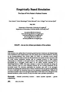
the true mean for all replications, and the coverage is defined as the number of confidence intervals that contain a divided by the total number of confidence intervals generated+ We expect 1s, 2s, and 3s coverages to correspond roughly to 68%, 95%, and 99+7% of the confidence intervals covering a+ The first model we consider is the M0M0` queue-length process+ This is a birth-death process X 5 $X~t! : t $ 0% that has birth rates l n 5 l and death rates µ n 5 nµ for n $ 0+ In this case, X lives in a discrete state space+ It is well known that if X~0! 5 0, then X~t! is Poisson distributed with parameter ~l~1 2 exp~ µt!!0µ!+ Suppose we are interested in estimating the quantity a 5 E~X~t!!+ This corresponds to setting f ~x! 5 x and G~dx! 5 dt ~dx! in Eq+ ~1+1!+ Then a 5 E f ~X~t!! 5

l~1 2 exp~2µt!! + µ

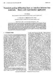
Let c be the total computer budget and c1 5 rc ~r [ ~0,1!!+ The coupling used here is the independent coupling; we simulate the two processes independently until they couple+ Tables 1 and 2 compare the absolute errors, the mean square errors, and the coverage of the conventional estimator, a0 ~c!, the coupling-based estimator, a1~c!, and the empirically based coupling estimator, a2 ~c!+ The performance of the conventional estimator, as measured by the mean square error, degrades as t gets large, whereas the performance of the coupling-based estimator a1~c! improves as t r `+ It should come as no surprise that the variance of a1~c! goes to zero as t r `+ The empirically based coupling estimator a2 ~c! does not show significant change as t r `+ As discussed in the previous section, the variance associated with the estimator, s 2, converges to a constant as t r `+ Since the empirically based coupling estimator does not degrade, its performance is better than the conventional estimator for large t as shown in the experiments+ In terms of confidence intervals coverage, all three estimators give reasonable results+ The next model we study is the M0M01 waiting time process, W 5 $W~i! : i $ 0% with traffic intensity r , 1+ It is an irreducible, positive recurrent, discrete-time Markov chain living on a continuous state space, R1+ Here we are interested in estimating EW~n! for n . 0+ Again, we use independent coupling, with coupling time Ti ~c! 5 inf $m $ 0 : W11 ~c, m! 5 W12 ~c, m! 5 0%+ Since the aperiodic chain W visits state 0 infinitely often, we have P~Ti ~c! , `! 51+ The expected value EW~n! can be obtained as follows+ Let p be the probability that the existing customer will be served before a new customer arrives+ So, p 5 µ0~l 1 µ!; the corresponding probability that a new customer will arrive before an existing customer is served is q 51 2 p+ Let Pij be the probability that, if there are currently i customers in the system, there will be j customers in the system just prior to the arrival of the next customer+ Therefore, for each i,

t

Estimator

Replications

c

r

Error

MSE

1s

2s

3s

0+5 0+5 0+5

a0 a1 a2

100 100 100

20000 20000 20000

0 0 0+44

20+000075670 20+000178395 20+000157398

0+000006657 0+000005022 0+000024756

0+54 0+68 0+70

0+93 0+99 0+97

0+99 1+00 0+99

1+0 1+0 1+0

a0 a1 a2

100 100 100

20000 20000 20000

0 0 0+40

0+000177221 20+000006267 20+00015954

0+000013352 0+000006702 0+00007541

0+76 0+68 0+68

0+99 0+95 0+92

0+99 0+99 0+99

2+0 2+0 2+0

a0 a1 a2

100 100 100

20000 20000 20000

0 0 0+51

20+001160358 0+000154736 0+00029991

0+000035513 0+000003761 0+00008595

0+76 0+68 0+65

0+95 0+95 0+92

1+00 0+99 0+99

5+0 5+0 5+0

a0 a1 a2

100 100 100

20000 20000 20000

0 0 0+61

0+000993973 0+000014310 0+00052970

0+000127154 0+000000296 0+00008346

0+72 0+64 0+66

0+94 0+90 0+95

1+00 0+99 0+98

7+0 7+0 7+0

a0 a1 a2

100 100 100

20000 20000 20000

0 0 0+61

20+000922645 20+000039807 0+001339981

0+000211488 0+000000043 0+000083268

0+61 0+65 0+64

0+93 0+91 0+96

1+00 0+95 0+99


Table 1. M0M0` Queue-Length Process with l 5 0+5, µ 5 1+0

159

160

Table 2. M0M0` Queue-Length Process with l 5 2+0, µ 5 1+0 Estimator

Replications

c

r

Error

MSE

1s

2s

3s

0+5 0+5 0+5

a0 a1 a2

100 100 100

20000 20000 20000

0 0 0+29

0+000988069 0+000220167 20+00200724

0+000020286 0+000085861 0+00018906

0+64 0+65 0+79

0+97 0+93 0+97

1+00 1+00 0+99

1+0 1+0 1+0

a0 a1 a2

100 100 100

20000 20000 20000

0 0 0+57

20+000526618 0+003797064 0+002258368

0+000072227 0+000086822 0+000299082

0+67 0+68 0+74

0+91 0+96 0+99

0+99 1+00 1+00

2+0 2+0 2+0

a0 a1 a2

100 100 100

20000 20000 20000

0 0 0+46

0+000167566 0+002803725 20+003322026

0+000132771 0+000073235 0+000462243

0+74 0+64 0+65

0+99 0+91 0+92

1+00 1+00 1+00

5+0 5+0 5+0

a0 a1 a2

100 100 100

20000 20000 20000

0 0 0+70

20+001049106 0+000505925 20+007038762

0+000409169 0+000004452 0+000381976

0+73 0+56 0+60

0+95 0+91 0+90

1+00 0+97 0+98

7+0 7+0 7+0

a0 a1 a2

100 100 100

20000 20000 20000

0 0 0+71

20+005216124 0+000116769 20+004858809

0+000756011 0+000000512 0+000265057

0+68 0+61 0+70

0+97 0+86 0+95

0+99 0+94 0+99


t


Pij 5

5

if j 5 i 1 1 if j . i 1 1

q 0

if i $ j $ 1

p i2j11 q p

161

if j 5 0+

i11

Now we generate EW~n! iteratively+ Let djN denote the probability that when the Nth customer arrives in the system, there will already be j customers present+ Setting d00 51, the vector $djN : j $ 0% may be computed recursively in N+ Then, the expected waiting time for the Nth arriving customer is given by E~W~N !! 5

1 µ

N21

( jd

N j

+

j51

The experimental results for this model can be found in Tables 3 and 4+ Again the performance ~measured in mean square error! of the conventional estimator degrades as t r `+ The coupling-based estimator continues to have superior performance for large t+ The empirically based coupling estimator a2 ~c! dominates the conventional estimator as t r `, since it does not change significantly as t gets large+ Note that the confidence interval coverages for the coupling-based estimator a1~c! are not close to their nominal values+ The reason is that the tiny variances contribute to a relatively large skewness; this creates small-sample difficulties in the normal approximation+ 4. PROOFS Proof of Proposition 1: For any x [ S, 7P~X~t! [ {6X~0! 5 x! 2 P~X~t! [ {!7 5 7Px ~X 2 ~t! [ {! 2 Px ~X 1 ~t! [ {!7 # Px ~T . t! r 0 as t r `+ On the other hand, 7p~{! 2 P~X~t! [ {!7 #

E

p~dx!7P~X~t! [ {6X~0! 5 x! 2 P~X~t! [ {!7,

S

so 7p~{! 2 P~X~t! [ {!7 r 0 as t r ` also+ Hence, Eq+ ~2+3! follows+ Furthermore, for any bounded f, Eq+ ~2+3! implies that E @ f ~X~t!!6X~0! 5 x# r E f ~X * ~0!! as t r `+ We may then invoke Theorem 1 of Glynn @6# to conclude that X is Harris n recurrent+ Proof of Theorem 1: Let R i ~c! 5

E

@0,Ti ~c!!

@ f ~X i1 ~c, t!! 2 f ~X i 2 ~c, t!!#G~dt!+

162

Table 3. M0M01 Waiting Time Process with l 5 0+2, µ 5 1+0 Estimator

Replications

c

r

Error

MSE

1s

2s

3s

1+0 1+0 1+0

a0 a1 a2

100 100 100

20000 20000 20000

0 0 0+10

20+00027 0+00352 20+00044

0+00002 0+00005 0+00035

0+64 0+46 0+63

0+94 0+81 0+94

1+00 0+95 0+98

2+0 2+0 2+0

a0 a1 a2

100 100 100

20000 20000 20000

0 0 0+42

20+00066 0+00322 20+00113

0+00005 0+00004 0+00015

0+64 0+48 0+66

0+94 0+77 0+96

1+00 0+93 0+99

5+0 5+0 5+0

a0 a1 a2

100 100 100

20000 20000 20000

0 0 0+47

0+00084 0+00051 20+00110

0+00016 0+00001 0+00014

0+66 0+52 0+72

0+93 0+80 0+90

1+00 0+98 0+97

7+0 7+0 7+0

a0 a1 a2

100 100 100

20000 20000 20000

0 0 0+58

20+00154 20+00001 0+00084

0+00019 0+00000 0+00016

0+65 0+49 0+63

0+96 0+93 0+92

1+00 0+97 0+98

10+0 10+0 10+0

a0 a1 a2

100 100 100

20000 20000 20000

0 0 0+60

0+00089 0+00005 20+00174

0+00035 0+00000 0+00014

0+63 0+23 0+55

0+93 0+67 0+88

0+99 0+79 0+98


N

N

Estimator

Replications

c

r

5+0 5+0 5+0

a0 a1 a2

100 100 100

20000 20000 20000

0 0 0+12

7+0 7+0 7+0

a0 a1 a2

100 100 100

20000 20000 20000

10+0 10+0 10+0

a0 a1 a2

100 100 100

20+0 20+0 20+0

a0 a1 a2

50+0 50+0 50+0

a0 a1 a2

Error

MSE

1s

2s

3s

0+00047 0+04128 0+00321

0+00051 0+00240 0+00513

0+66 0+17 0+58

0+94 0+41 0+95

0+99 0+70 1+00

0 0 0+54

20+00284 0+03006 20+00820

0+00087 0+00146 0+00264

0+63 0+29 0+75

0+97 0+60 0+92

1+00 0+86 1+00

20000 20000 20000

0 0 0+59

0+00129 0+01532 20+00473

0+00136 0+00066 0+00238

0+66 0+40 0+69

0+97 0+78 0+93

0+99 0+93 0+99

100 100 100

20000 20000 20000

0 0 0+72

0+00555 0+00497 0+00554

0+00361 0+00022 0+00240

0+63 0+49 0+68

0+95 0+79 0+95

0+98 0+91 0+99

100 100 100

20000 20000 20000

0 0 0+53

20+01112 20+00007 0+00647

0+00724 0+00001 0+00282

0+66 0+2 0+64

0+97 0+6 0+97

0+99 0+68 1+00


Table 4. M0M01 Waiting Time Process with l 5 0+5, µ 5 1+0

163

164


Note that 7P~R 1 ~c! [ {6X ! 2 P * ~R [ {!7

* E ~p ~dx! 2p~dx!!P ~R [ {! * # 7p 2 p7 r 0 a+s+

5

c

x

c

S

as c r `+ Furthermore, E~R 12 ~c!6X ! 5

E E

pc ~dx!Ex R 2

S

5

pc ~dx!g2 ~x! r

S

E

p~dx!g2 ~x! 5 E * R 2 a+s+

S

as c r `, so $R 12 ~c! : c . 0% is a uniformly integrable family of r+v+’s+ As a consequence, we may apply the Lindeberg–Feller CLT ~see Chung @2, p+ 205# ! path-bypath to conclude that P

S

1

{lc2}

#lc2

i51

D

( ~R ~c! 2 E~R ~c!6X !! # {6X i

1

as c r `+ Also, for e . 0, P~N~c2 !! , lc2 ~1 2 e!6X ! # P #P

S S

n P~s2 N~0,1! # {! a+s+

D

[lc2 ~12e!]

(

xi ~c! . c2 6X

i51 [lc2 ~12e!]

(

(4.8)

~ xi ~c! 2 E @ x1 ~c!6X # !

D

i51

. c2 2 [lc2 ~1 2 e!]E @ x1 ~c!6X #6X #

var~ x1 ~c!6X ![lc2 ~1 2 e!] r 0 a+s+ ~c2 2 [lc2 ~1 2 e!]E @ x1 ~c!6X # ! 2

as c r `, by virtue of A3 and A5+ Similarly, P~N~c2 !! . lc2 ~1 1 e!6X ! r 0 a+s+ as c r `+ So, P~6N~c2 ! 2 lc2 6 . ec2 6X ! r 0 a+s+

(4.9)

as c2 r `+ Furthermore, because R 1~c!, R 2 ~c!, + + + are independent conditional on X, Kolmogorov’s Inequality implies that for e . 0,

S* (

N~c2 !

{lc2}

P

i51

#P

~R i ~c! 2 E~R i ~c!6X !! 2

S

( ~R ~c! 2 E~R ~c!6X !! 6 . e!c i

i

i51

max 3

1#6 j 6#e c2

*

{lc}1j

(

i5{lc}

1 P~6N~c2 ! 2 lc2 6 . e 3 c2 6X ! #

var~R 1 ~c!6X !e 3 c2 e 2 c2

*D

~R i ~c! 2 E~R i ~c!6X !! 6 . e!c2 X

1 P~6N~c2 ! 2 lc2 6 . e 3 c2 6X !+

2

* XD


165

If we let c r `, followed by letting e r 0 ~and apply A3, A4, Eq+ ~4+1!, and Eq+ ~4+2!!, we may conclude that P

S

D

N~c2 !

1

( ~R ~c! 2 E @R ~c!6X#! # {6X i

i

i51

#lc2

n P~s2 N~0,1! # {! a+s+

as c r `+ Utilizing Eq+ ~4+2! again, we find that

SS

P !c

N~c2 !

1 N~c2 !

nP

S

( ~R ~c! 2 E @R ~c!6X # ! i

i

i51

s2

% ~1 2 r!l

D

S S

N~c2 !

1 N~c2 !

# {6X

N~0,1! # { a+s+

as c r `+ Hence, for each u, E exp iu!c

D D

( ~R ~c! 2 E @R ~c!6X # ! j

1

j51

DD S 6X r exp

2u 2 s22 2~l~1 2 r!!

D

as c r `+ Consequently, noting that Gj ~c! 5 R j ~c! 2 E @R 1 ~c!6X # 1

E

pc ~dx!k~x!,

S

we get E exp~iu!c~a~c! 2 a!!

S S ( H S S E S S

5 E exp iu!c

5 E exp iu!c

1 N~c2 ! 1 c1

N~c2 !

~R j ~c! 2 E @R 1 ~c!6X # ! 1

j51

c1

k~x!pc ~dx! 2 a

0

1 3 E exp iu!c N~c2 !

S

r exp 2

E

pc ~dx!k~x! 2 a

S

DD

N~c2 !

( ~R ~c! 2 E @R ~c!6X # ! j

j51

s22 u 2 s12 u 2 2 2r 2l~1 2 r!

D

1

DD

DDJ

as c r `, proving the theorem+

n

Proof of Theorem 2: Using A7, a proof very similar to that of Theorem 1 establishes that !c~a1 ~c! 2 a, + + + , am ~c! 2 a! n s!m~N1 ~0,1!, + + + , Nm ~0,1!! as c r `, where N1~0,1!, + + + , Nm ~0,1! are i+i+d+ normally distributed r+v+’s with mean zero and unit variance+ The conclusion follows from an application of the continun ous mapping principle ~see Billingsley @1# !+

166


Proof of Proposition 2: Note that sup B

* E 1 c1

c1

5 sup B

#

I ~X~s! [ B! ds 2 p~B!

0

*(

y[B

1 c1

(* E

y[S

52

(

1 c1

y[S

S

c1

E

c1

*

I ~X~s! 5 y! ds 2 p~ y!

0

I ~X~s! 5 y! ds 2 p~ y!

0

p~ y! 2

1 c1

E

c1

*

*

DS

I ~X~s! 5 y! ds I p~ y! .

0

1 c1

E

0

c1

D

I ~X~s! 5 y! ds +

The summands are dominated by 2p~ y! ~which is summable! and converge to zero a+s+ Applying the dominated convergence theorem path-by-path leads to the conclusion that the above sum converges to zero a+s+ as c r `+ n Proof of Proposition 3: Let p~ y! 5

E

p~dx!p~x, y!,

1 c1

E

S

pc ~ y! 5

c1

p~X~s!, y! ds+

0

By stationarity of p, p~B! 5

E E

p~dx!

S

5

E

p~x, y!h~dy!

B

p~ y!h~dy!+

B

Also, pc ~B! 5

E

pc ~ y!h~dy!+

B

Fix e . 0+ Because h and p are tight @1#, there exists a compact set K such that h~K c ! , e, and p~K c ! , e+ Set 7p7 5 sup $ p~x, y! : x, y [ S %+ Note that 7p7 $ p~ y!, 7p7 $ pc ~ y! for c . 0, y [ S+ Since p is necessarily uniformly continuous on K 3 K, there exists y1 , y2 , + + + , yl [ K such that for each y [ K, there is a yi for which 6 p~x, y! 2 p~x, yi !6 , e


167

for x [ K+ Hence, sup 6 pc ~ y! 2 p~ y!6 y[K

# sup

y[K

*E *E

p~x, y!

K

# max

1#i#l

5 max

1#i#l

S E S E

p~x, yi !

K

* E E 1 c1

c1

c1

1 c1

D* D*

I ~X~s! [ dx! ds 2 p~dx!

0

1 c1

c1

1 e7p7

I ~X~s! [ dx! ds 2 p~dx!

0

1 3e7p7

p~X~s!, yi !I ~X~s! [ K ! ds

0

*

p~x, yi !I ~x [ K !p~dx! 1 3e7p7 r 3e7p7 a+s+

2

S

(4.10)

as c r `, by the law of large numbers for Harris processes ~applied to the finite collection of sample functions associated with y1 , + + + , yl !+ Then, sup 6pc ~B! 2 p~B!6 5 sup B

B

#

E E

* E p ~ y!h~dy! 2E p~ y!h~dy! * c

B

B

6 pc ~ y! 2 p~ y!6h~dy!

S

#

6 pc ~ y! 2 p~ y!6h~dy! 1 e7p7

K

# sup 6 pc ~ y! 2 p~ y!6 1 e7p7+ y[K

By virtue of Eq+ ~4+10!, we conclude that lim sup 6pc ~B! 2 p~B!6 # 4e7p7+

cr`

B

Since e was arbitrary, this proves the result+

n

References Billingsley, P+ ~1968!+ Convergence of probability measure. New York: John Wiley+ Chung, K+L+ ~1974!+ A course in probability theory. New York: Academic Press+ Devroye, L+ ~1985!+ Nonparametric density estimation: The L1 view. New York: John Wiley+ Fox, B+L+ & Glynn, P+W+ ~1989!+ Estimating discounted costs+ Management Science 35: 1297–1325+ Glynn, P+W+ ~1989!+ A GSMP formalism for discrete-event systems+ Proceedings of the IEEE 77: 14–23+ 6+ Glynn, P+W+ ~1994!+ Some topics in regenerative steady state simulation+ Acta Applicandae Mathematicae 34: 225–236+ 7+ Glynn, P+W+ & Wong, E+W+ ~1996!+ Efficient simulation via coupling+ Probability in the Engineering and Informational Sciences 10: 165–186+ 8+ Lindvall, T+ ~1992!+ Lectures on the coupling method. New York: John Wiley+ 1+ 2+ 3+ 4+ 5+