Transition from single-domain to vortex state in soft magnetic cylindrical nanodots W. Scholz,1, ∗ K. Yu. Guslienko,2, † V. Novosad,3 D. Suess,1 T. Schrefl,1 R. W. Chantrell,2 and J. Fidler1 1
Vienna University of Technology, Wiedner Hauptstrasse 8-10/138, A-1040 Vienna, Austria 2
Seagate Research, 1251 Waterfront Place, PA 15222-4215
3
Materials Science Division, Argonne National Laboratory, 9700 S. Cass Ave., Argonne, IL 60439 (Dated: February 18, 2003)
Abstract We have investigated the magnetic properties of submicron soft magnetic cylindrical nanodots using an analytical model as well as three dimensional numerical finite element simulations. A detailed comparison of the magnetic vortex state shows the differences between these two models. It appears that the magnetic surface charges play a crucial role in the equilibrium magnetization distribution especially for shifted vortices. Finally, the magnetic phase diagram for soft magnetic particles with varying aspect ratio is presented.
1
I.
INTRODUCTION
The recent advances in microfabrication techniques have stimulated interest in the properties of submicron sized patterned magnetic elements.1,2 Promising applications include magnetic random access memory, high-density magnetic recording media, and magnetic sensors.3 However, in order to exploit the special behavior of magnetic nanoelements it is necessary to study and understand their fundamental properties. We have studied the static properties of cylindrical magnetic nanodots of different sizes and aspect ratios with analytical models and numerical finite element (FE) simulations, especially magnetic vortex states. Direct experimental evidence for the existence of these magnetic vortex states has been found by the method of magnetic force microscopy. Shinjo and coworkers4 have used Magnetic Force Microscopy (MFM) to characterize magnetic nanodots of permalloy (Ni80 Fe20 ) with a thickness of 50 nm and a radius between 300 nm and 1 µm, for example. The hysteresis loops of magnetic nanodots have been measured by vibrating sample magnetometer2 and magneto-optical methods5 and successfully identified single domain and vortex states. Furthermore, these magnetic vortex states are an interesting object for high frequency magnetization dynamics6 experiments, which are important for high-density magnetic recording media, where high-frequency field pulses of the magnetic write head store the information by reversing the magnetization. In Sec. II the analytical rigid vortex model is outlined and in Sec. III we compare its results with finite element micromagnetic simulations. Then the hysteresis curve of a magnetic nanodot and the different contributions to the total energy are discussed in Sec. IV. The average magnetization and surface charges are discussed in Sec. V and VI. Finally, the phase diagram of magnetic ground states compares the results of the analytical model, numerical FE simulations and experimental results in Sec. VII.
II.
THE ANALYTICAL RIGID VORTEX MODEL
The rigid vortex model assumes a “rigid vortex”, which does not change its shape in an external field. Together with a certain magnetization distribution it gives an approximation for the magnetization distribution of a curling state (vortex state) in a fine cylindrical
2
a
R
z y x
L
FIG. 1: Geometry of a flat cylindrical nanodot.
particle. An analytical model for the magnetization distribution M(x) in zero field has been developed using a variational principle by Usov and coworkers.7,8 It is split into two parts (cf. Figs. 1, 2). The first part describes the magnetization in the core of the vortex (r ≤ a, a is the vortex core radius), which is defined by Mz 6= 0:
Mx = My =
− a22ar sin ϕ +r2 2ar a2 +r2
q
Mz = − 1 −
cos ϕ 2ar a2 +r2
(1) ,
where r, ϕ are the polar coordinates. The other part describes the magnetization outside the core (r > a): Mx = − sin ϕ My = cos ϕ Mz =
(2)
0
The transition between the vortex core and the rest of the cylindrical dot is continuous but the function Mz (r) is not differentiable at r = a. The parameter a can be found from minimization of the total magnetic energy of the dot. Eqs. 1 and 2 represent a twodimensional radially symmetric vortex model, which has the following properties: 1) In equilibrium (in zero external field) there are surface charges on the top and bottom surface within the vortex core. 2) Side surface charges are equal to zero on the circumference of the dot. 3) There are no volume charges. Upon applying an in-plane magnetic field the vortex is shifted from the dot center perpendicularly to the field. As a result, side surface charges are induced. In this work we have checked the applicability of Usov’s analytical vortex model and the rigid vortex model in an external field numerically. In addition we have studied the dependence of M (r) on the z-coordinate (along the thickness of the nanodot). 3
0 Mz/Ms
-0.2 -0.4 -0.6 -0.8 -1 -1
Usov’s model FE equilib.
-0.5
0 r/R
0.5
1
FIG. 2: Comparison of the profiles of Mz between the analytical model and the remanent state obtained by the finite element simulation. The profile has been taken along the x-axis through the center of the nanodot, which has an aspect ratio of L/R = 20 nm/100 nm = 0.2. III.
THE FINITE ELEMENT MODEL
The numerical computer simulations have been carried out using a 3D dynamic hybrid finite element/boundary element micromagnetic code with a static scalar potential for the calculation of the demagnetizing field and a preconditioned backward differentiation formula for the time integration of the Landau-Lifshitz equation of motion.9 In our calculations we have assumed the following material parameters for permalloy (Ni80 Fe20 ): Ms = 8 × 10⁵ A/m(8 × 102 G), A = 13 × 10−12 J/m(1.3 × 10−6 erg/cm), anisotropy has been neglected. Thus, the exchange length is lex =
q
2A/(µ0 Ms2 ) = 5.7 nm.
Fig. 2 shows the Mz profile of a nanodot with a radius of 100 nm and a thickness of 20 nm as obtained by the analytical vortex and the finite element model in zero field in equilibrium. The results show that the vortex core is approximately 54% larger (18.5 nm) than that assumed by the analytical vortex model (12 nm), if the core radius is defined by the first Mz = 0 crossover from the center. Furthermore there is a region with Mz < 0 outside the vortex core. Thus, we find negative surface charges in the core of the vortex, which are surrounded by positive surface charges. Only outside of approximately half the radius (50 nm) almost all surface charges disappear. In addition we find a radial component of the magnetization, which is greatest at about half the vortex core radius (Fig. 3). Nevertheless, as we show here below, the analytically calculated energy terms associated with a vortex core are in good agreement with numerical micromagnetic simulations.
4
Mr/Ms
0.15 0.1 0.05 0 -0.05 -0.1 -0.15 -1
top center bottom
-0.5
0 r/R
0.5
1
FIG. 3: Mr line scan across the nanodot at its top, in the center, and at the bottom. units: J/m3
Magnetostatic Exchange Total energy
energy
energy
Analytical vortex model 432.1
5356
5788
FE approx.
417.0
5341
5758
FE error
-3.5 %
-0.28 %
-0.52 %
FE simulation (equilib.) 387.1
5150
5537
difference FE - analytical -10.42 %
-3.85 %
-4.35 %
TABLE I: Comparison of the energies obtained by the analytical vortex model and the numerical FE simulation.
Similar magnetization profiles have been calculated by Buda et al.10 for circular Co dots with perpendicular magnetocrystalline anisotropy. There the uniaxial anisotropy leads to a stripe domain structure (circles around the vortex core), which gets more pronounced as the dot thickness increases.
IV.
ENERGY AND HYSTERESIS
Next the exchange and magnetostatic energies of the vortices are compared. The formulas for the analytical vortex model have been derived by Usov et al.7,8 The finite element results are in good agreement with the analytical results (the discretization error of the total energy is just -0.52 %) and it is shown in Table I, that the energy of the equilibrium magnetization distribution, which has been found with the FE model, is more than 4% smaller than that of the analytical vortex model. Fig. 4 shows the hysteresis curve for a circular nanomagnet with an in-plane external
5
Mx/Ms
1
5(b)
5(a)
0.5 0
6(a)
-0.5 6(b)
decr. field incr. field
-1 -50
0 Hext (kA/m)
50
FIG. 4: Hysteresis curve of a nanodot with L/R = 20 nm/100 nm = 0.2 for an in-plane external field. The circles mark the position on the hysteresis curve at which the snapshots in Figs. 5 and 6 have been taken.
field. For very high external fields (applied in the plane of the nanodot), the magnetization is almost uniform and parallel to the external field (Fig. 5(a)). As the field decreases (solid line in Fig. 4) the magnetization distribution becomes more and more non-uniform, which is caused by the magnetostatic stray field. Upon further decrease of the external field, the symmetry of the magnetization distribution breaks and at the nucleation field (about 5 kA/m in our example) a “C” state (Fig. 5(b)) develops. As it was shown in Guslienko et al. 11 , this type of nucleation mode is typical for dots with small diameters, whereas the “Sshape” spin instability mode is expected for bigger elements. However, the “C” state is only a metastable state. It leads to the nucleation of a vortex, which quickly moves towards its equilibrium position (close to the center of the nanodot). As a result we find a sudden drop in the average magnetization. When the external field is reduced to zero the vortex moves into the center of the nanodot (Fig. 6(a)). If the external field is increased in the opposite direction, the vortex is forced out of the center of the dot. For about −70 kA/m the vortex is pushed out of the nanodot (annihilation: Fig. 6(b)) and we find the second jump in the hysteresis curve to (almost) saturation. At the annihilation field the minimum of the total energy turns into a saddle point or maximum, which makes the vortex state unstable. This happens due to an increase in the magnetostatic energy as the vortex approaches the edge, because the surface charge density on the circumference increases. As a result, the systems proceeds towards the next energy minimum, which is found in the state with homoegeneous magnetization distribution. This stability analysis is used for the analytical calculation of the annihilation field.12 6
(a)
H ext
(b)
FIG. 5: Leaf state (a) (for high external in-plane fields) and “C” state (b) (develops before the vortex nucleation).
(a)
H ext
(b)
FIG. 6: Centered vortex (a) in zero field and far shifted vortex (b) before annihilation.
This characteristic behavior has also been found experimentally using Hallmicromagnetometry by Hengstmann et al.13 , who measured the stray field of individual permalloy disks using a sub-µm Hall magnetometer. The hysteresis loops of arrays of Supermalloy nanomagnets have been measured by Cowburn et al.5 using the Kerr effect. Their characteristic loop shape has then been used to identify the single-domain in-plane and the vortex phase. The rigid vortex model can describe very well the susceptibility, magnetization distribution, and vortex annihilation field for low fields as well as the vortex nucleation field for a wide range of dot sizes.11,14–16 However, expecially for larger dot radii the experimentally and numerically observed nucleation fields appear to be bigger than those predicted by the rigid vortex model. This is due to the fact, that more complex nucleation modes (including “S-states”) have to be taken into account, but they are not included in the rigid vortex model.17 In Fig. 7 the total energy is plotted as a function of the external field for the branch of decreasing field of the hysteresis curve. The solid line indicates the hysteresis branch for 7
Energy (arb. units)
0.04
decr. field incr. field
0.02 0 -0.02 -0.04 -50
0 Hext (kA/m)
50
FIG. 7: Total energy as a function of the external field for both branches (solid line for decreasing field - dashed line for increasing field) of the hysteresis loop.
decreasing external field and the dashed line corresponds to increasing field. For very high fields we have an almost uniformly magnetized nanodot. As the external field decreases the total energy increases linearly due to the homogeneous magnetization distribution and the dominant contribution of the Zeeman term. The dashed curve for positive field values indicates the total energy for the vortex state. At the intersection of the solid and the dashed line (at a value of about 35 kA/m for the external field) the vortex state and the uniform magnetization have equal energy. However, they are separated by an energy barrier due to the magnetostatic energy, which in turn is caused by the stray field on the circumference of the nanodot as the vortex is pushed out of the center. Thus, the vortex state is a metastable state for external fields higher than 35 kA/m and the uniform state is metastable for external fields below 35 kA/m. The field dependence of exchange and magnetostatic energy is given in Fig. 8. The exchange energy remains approximately constant for negative external fields until the annihilation field is reached. Since all the exchange energy is stored in the vortex core, this indicates that the vortex core remains undisturbed for even very large vortex shifts. For a twice large nanodot with R = 200 nm and L = 40 nm we find a nucleation field of 28 kA/m and an annihilation field of 84 kA/m. In general, the initial susceptibility, the vortex nucleation, and the annihilation fields depend on the dot’s saturation magnetization Ms and should scale universally as a function of the dimensionless dot-aspect ratio L/R.11,14
8
Energy (arb. units)
0.06 0.05 0.04 0.03 0.02 0.01 0
exchange magnetostatic sum
-50
0 Hext (kA/m)
50
FIG. 8: Exchange and magnetostatic energy and their sum as a function of the external field (for decreasing external field).
0 Mz/Ms
-0.2 -0.4 -0.6 -0.8 -1 -1
-0.5
0 y/R
0.5
1
FIG. 9: Profiles of Mz along the y-axis through the center of the nanodot for a vortex moving in −y direction due to an external field increasing in x direction. V.
AVERAGE MAGNETIZATION
Fig. 9 shows profiles of Mz along the y-axis for different external fields. As a result, the vortex is shifted and the profile “moves” towards the circumference of the dot (|y/R| = 1). From this plot the position of the vortex core for a given external field has been extracted. The corresponding average magnetization hMx i is plotted in Fig. 10 (open circles). For symmetry reasons My is zero (the vortex is shifted along the y-axis, since we applied a field in x-direction). By integrating the magnetization distribution of the rigid vortex model over the surface of the nanodot the average magnetization hMx i has been calculated. The result is given in Fig. 10. We find very good agreement between the rigid vortex model and the finite element simulation. The small difference can be understood by considering small deviations of the magnetization distribution due to surface charges on the circumference (cf. section VI).
9
/Ms
0
FE rigid vortex
-0.2 -0.4 -0.6 -0.8 -1
-0.8
-0.6 -0.4 y/R
-0.2
0
FIG. 10: Comparison of hMx i as a function of the vortex displacement between the FE simulation and the rigid vortex model. y = 0 corresponds to a centered vortex, y = −0.78 is the maximum shift before vortex annihilation occurs in the FE simulation. VI.
CHARGE DENSITIES AND THE MAGNETOSTATIC FIELD
Another important aspect in comparison with the rigid vortex model is the magnetostatic energy and the surface charges, which generate the magnetostatic field. On the top and bottom circular surface the surface charges are proportional to Mz , because the normal vector n of the top and bottom is simply ez and −ez , respectively. However, on the circumference the normal vector is, of course, er . If an in-plane external field is applied, the vortex core is shifted perpendicular to the direction of the field (Fig. 6) towards the circumference of the nanodot. Thus, the magnetization does not form concentric circles (Mr = 0) around the dot axis any more and surface charges appear on the circumference. The surface charge densities on the circumference of the nanodot are given in Fig. 11 for different vortex core displacements. For small external fields and therefore small vortex displacements there is very good agreement between the rigid vortex model and the finite element simulation. As the external field increases more surface charges appear on the circumference of the nanodot. However, the rigid vortex model overestimates these surface charges. The values for the average magnetization is in good agreement, but the surface charge distribution is not. The reason is that the magnetization distribution close to the circumference is disturbed by the strong demagnetizing fields. As we further increase the external field and the vortex displacement this deviation becomes more and more pronounced. In addition, we also find some deviation in the center of the nanodot, which arises from a more “elliptical” shape of the magnetization distribution as the vortex is pushed towards
10
= -0.028 = -0.122 = -0.438 = -0.718
Div M/Ms
0.5 0 -0.5 -200
-100
0 ϕ (deg)
100
200
FIG. 11: Surface charge distribution on the circumference of the nanodot as a function of the polar angle. An in-plane external field shifts the vortex (cf. Fig. 12) and leads to surface charges on the circumference. The rigid vortex model (gray lines) overestimates the charge density as compared to the FE simulation (black lines).
FIG. 12: Contour plot of d = |MFE − Mrv |. Dark areas indicate good agreement of the magnetization distribution between the rigid vortex model (black cones) and the FE model (gray cones), lighter areas indicate larger differences.
the boundary. A contour plot of the difference between the magnetization distribution calculated by the FE simulation and the rigid vortex model d = |MFE − Mrv | is shown in Fig. 12 for Hext = 66.0 kA/m = 830 Oe, hMx i/Ms = −0.72, and b/R = −0.76. The light areas at the circumference and in the center of the nanodot indicate differences between the rigid vortex model and the FE simulation. In remanence, the demagnetizing field arising from the vortex structure is mainly concentrated in the vortex core (Fig. 13). It has a dominating z-component and a smaller radial component.
11
µ0Hdem (T)
0.4
Hz Hr
0.3 0.2 0.1 0 -1
-0.5
0 r/R
0.5
1
FIG. 13: Hzdem and Hrdem across the nanodot. VII.
PHASE DIAGRAM
A summary of the results of the equilibrium magnetization distribution of nanodots with different aspect ratios is given in the phase diagram in Fig. 14. The transition from the inplane magnetization to the vortex state is sharp, because this requires that the symmetry of the single domain state with (almost) homogeneous in-plane magnetization breaks in order to form the vortex state with cylindrical symmetry. The line separating the in-plane and out-of-plane remanent states has a slope of 1.8, which is in agreement with the simulations by Ross et al.2 and analytical calculations.18 Magneto-optical measurements of hysteresis curves5 also show a distinct change between these two regimes. The single domain particles retain high remanence and switch at very low fields, whereas a sudden loss in magnetization reducing the external field (cf. Fig. 4) is typical of a flux closure configuration (vortex state). However, the transition from the vortex to the perpendicular magnetization (parallel to the cylinder axis) is not well defined. The numerical experiments show a smooth transition from one state to the other. For decreasing dot aspect ratio, the magnetization starts to twist and exhibits very inhomogeneous magnetization distributions. So we have defined a magnetization distribution with Mz > 0.75 as being a perpendicular ground state. The two-dimensional analytical model cannot describe this transition properly, because it would require, that the dependence of the magnetization on the z-coordinate is taken into account. Nevertheless, the numerical results and the experimental data are in excellent agreement with analytical calculations of this phase diagram. The solid lines in Fig. 14 have been taken from the phase diagram presented in Metlov and Guslienko 19 . Experimental data have been obtained from arrays of soft magnetic cylindrical particles by Ross et al.2 The data of their Ni samples are also shown in Fig 14. The agreement with
12
out-of-plane (perpendicular) vortex/ multidomain
L/lex
15 10 5
(1) in-plane magn.
0 0
2
6
4
8
10
R/lex FIG. 14: Phase diagram of magnetic ground states (axis scaling in units of the exchange length). The data points indicated by the open symbols have been calculated with the FE model. The
◦
circles ( ) represent dots with lowest energy in the in-plane magnetization state, squares (2) those with perpendicular magnetization, and diamonds (3) dots in vortex/multidomain state. The experimental data have been taken from Ross et al.2 The crosses (×) indicate “Ni Type A” samples with out-of-plane (perpendicular) magnetization at remanence, the plus symbols (+) indicate “Ni Type B” samples with in-plane, and the asterisks (∗)“Ni Type C” samples with vortex or multidomain states, respectively. The experimental data nicely fit in the phase diagram with one exception, which is indicated by “(1)”. There, a remanent state with in-plane magnetization has been found, where a vortex state might be expected. The solid lines give the analytical equilibrium single-domain radius calculated by Metlov et al.19
the numerically calculated phase diagram is very good. Only one data point does not fit in. A remanent state with in-plane magnetization is found, where a vortex state might be expected. However, also the smooth transition from the perpendicular magnetization to the vortex (multidomain) state has been found. Note, that ignoring the existence of the vortex core in nanodots20 leads to an over-estimation of the total energy and, as a result, to wrong coordinates of the lines separating different magnetic states in soft magnetic cylindrical nanodots.
VIII.
CONCLUSIONS
A detailed comparison of the rigid vortex model for magnetic vortex states in soft magnetic nanodots with the finite element simulations has revealed some special features of the 13
magnetic vortex state. The magnetization distribution near the vortex core radius (r = a) deviates essentially from Usov’s analytical model. Especially a non-vanishing radial component Mρ has been found (Fig. 3). In addition to the magnetic surface charges in the core of the vortex, the finite element simulations have revealed a ring of weak surface charges with opposite sign around the core of the nanodot. The shape of the vortex core and its exchange energy have been found to be very stable (“rigid”) even for large vortex shifts in an external field. However, the surface charges on the circumference of the nanodot are overestimated by the rigid vortex model, because the magnetization distribution is distorted from the perfectly circular shape by the magnetostatic stray field. As a result, the surface charges and the magnetostatic energy are reduced as compared to the rigid vortex model. Finally, the phase diagram of magnetic ground states shows sharp transitions from the “in-plane” state to the perpendicular magnetization distribution and the magnetic vortex state, whereas the transition from the perpendicular magnetization to the magnetic vortex state is not well defined.
Acknowledgments
Work in Vienna was supported by the Austrian Science Fund, Y-132 PHY. Work at ANL was supported by the US Department of Energy, BES Materials Science under contract W-31-109-ENG-38. The authors would like to thank M. Grimsditch for helpful discussions. R. W. Chantrell would like to acknowledge Robert Shull for handling the editorial process including the anonymous review procedure.
∗
Electronic address:
[email protected]; URL: http://magnet.atp.tuwien.ac. at/scholz/
†
[email protected]
1
C. A. Ross, Annu. Rev. Mater. Res. 31, 203 (2000).
2
C. A. Ross, M. Hwang, M. Shima, J. Y. Cheng, M. Farhoud, T. A. Savas, H. I. Smith, W. Schwarzacher, F. M. Ross, M. Redjdal, et al., Phys. Rev. B 65, 144417 (2002).
3
R. P. Cowburn, J. Phys. D: Appl. Phys. 33, R1 (2000).
4
T. Shinjo, T. Okuno, R. Hassdorf, K. Shigeto, and T. Ono, Science 289, 930 (2000).
14
5
R. P. Cowburn, D. K. Koltsov, A. O. Adeyeye, M. E. Welland, and D. M. Tricker, Phys. Rev. Lett. 83, 1042 (1999).
6
V. Novosad, M. Grimsditch, K. Y. Guslienko, P. Vavassori, Y. Otani, and S. D. Bader, Phys. Rev. B 66, 052407 (2002).
7
N. A. Usov and S. E. Peschany, J. Magn. Magn. Mater. 118, L290 (1993).
8
N. A. Usov and S. E. Peschany, Fiz. Met. Metalloved (transl.: The Physics of Metals and Metallography) 12, 13 (1994).
9
D. Suess, V. Tsiantos, T. Schrefl, J. Fidler, W. Scholz, H. Forster, R. Dittrich, and J. J. Miles, J. Magn. Magn. Mater. 248, 298 (2002).
10
L. D. Buda, I. L. Prejbeanu, M. Demand, U. Ebels, and K. Ounadjela, IEEE Trans. Magn. 37, 2061 (2001).
11
K. Y. Guslienko, V. Novosad, Y. Otani, H. Shima, and K. Fukamichi, Phys. Rev. B 65, 024414 (2001).
12
K. Y. Guslienko and K. L. Metlov, Phys. Rev. B 63, 100403(R) (2001).
13
T. M. Hengstmann, D. Grundler, C. Heyn, and D. Heitmann, J. Appl. Phys. 90, 6542 (2001).
14
K. Y. Guslienko, V. Novosad, Y. Otani, H. Shima, and K. Fukamichi, Appl. Phys. Lett. 78, 3848 (2001).
15
M. Schneider, H. Hoffmann, and J. Zweck, Appl. Phys. Lett. 77, 2909 (2000).
16
A. Fernandez and C. J. Cerjan, J. Appl. Phys. 87, 1395 (2000).
17
V. Novosad, K. Guslienko, H. Shima, Y. Otani, K. Fukamichi, N. Kikuchi, O. Kitakami, and Y. Shimada, IEEE Trans. Magn. 37, 2088 (2001).
18
A. Aharoni, J. Appl. Phys. 68, 2892 (1990).
19
K. L. Metlov and K. Y. Guslienko, J. Magn. Magn. Mater. 242-245, 1015 (2002).
20
J. d’Albuquerque e Castro, D. Altbir, J. C. Retamal, and P. Vargas, Phys. Rev. Lett. 88, 237202 (2002).
15