Translation from the Quantified Implicit Process Flow Abstraction in

Translation from the Quantified Implicit Process Flow Abstraction in SBGN-PD Diagrams to Bio-PEPA Illustrated on the Cholesterol Pathway Laurence Loewe1 , Maria Luisa Guerriero1 , Steven Watterson1,2 , Stuart Moodie3 , Peter Ghazal1,2 , and Jane Hillston1,3 1

Centre for System Biology at Edinburgh, King’s Buildings, The University of Edinburgh, Edinburgh EH9 3JD, Scotland [email protected], [email protected], 2 Division of Pathway Medicine, The University of Edinburgh [email protected], [email protected] 3 School of Informatics, The University of Edinburgh [email protected], [email protected]

Abstract. For a long time biologists have used visual representations of biochemical networks to gain a quick overview of important structural properties. Recently SBGN, the Systems Biology Graphical Notation, has been developed to standardise the way in which such graphical maps are drawn in order to facilitate the exchange of information. Its qualitative Process Description (SBGN-PD) diagrams are based on an implicit Process Flow Abstraction (PFA) that can also be used to construct quantitative representations, which facilitate automated analyses of the system. Here we explicitly describe the PFA that underpins SBGN-PD and define attributes for SBGN-PD glyphs that make it possible to capture the quantitative details of a biochemical reaction network. Such quantitative details can be used to automatically generate an executable model. To facilitate this, we developed a textual representation for SBGN-PD called “SBGNtext” and implemented SBGNtext2BioPEPA, a tool that demonstrates how Bio-PEPA models can be generated automatically from SBGNtext. Bio-PEPA is a process algebra that was designed for implementing quantitative models of concurrent biochemical reaction systems. The scheme developed here is general and can be easily adapted to other output formalisms. To illustrate the intended workflow, we model the metabolic pathway of the cholesterol synthesis. We use this to compute the statin dosage response of the flux through the cholesterol pathway for different concentrations of the enzyme HMGCR that is inhibited by statin.

1

Introduction

Biologists are constantly searching for strategies that help them to understand the complexity of life. Navigating the functional molecular interactions within cells has proven to be an increasing challenge since molecular biological research is filling databases with detailed knowledge about the molecular mechanics of life. A wide variety of schemes has been developed to represent such knowledge, ranging from textual representations that resemble chemical reactions (e.g. Dizzy [42]) or reaction rules (e.g.

BioNetGen, Kappa-calculus [13, 12, 24]) through XML-based standards like SBML [25] to graphical notations (e.g. [29, 43, 28, 38, 15, 33]). Graphical maps of biochemical reaction networks are proving to be powerful tools for facilitating an overview of the interactions of particular molecules. Recently the Systems Biology Graphical Notation (SBGN) has emerged as a standard for drawing such reaction diagrams [33, 32]. The objective is to provide molecular systems biologists with an easily understandable description of the system by generating consistent maps across different editing tools (e.g. CellDesigner [18], Cytoscape [11], Edinburgh Pathway Editor [46], JDesigner [44]). Like electronic circuit diagrams, they aim to unambiguously describe the structure of a complex network of interactions using graphical symbols. To achieve this requires a collection of symbols and rules for their valid combination. The SBGN Process Description, SBGN-PD, is a visual language with a precise grammar that builds on an underlying abstraction as the basis of its semantics (see p.40 [33]). We call this underlying abstraction for SBGN-PD the “Process Flow Abstraction” (PFA). It describes biological pathways in terms of processes that transform elements of the pathway from one form into another. The usefulness of an SBGN-PD description critically depends on the faithfulness of the underlying PFA and a tight link between the PFA and the glyphs used in diagrams. The graphical nature of SBGN-PD allows only for qualitative descriptions of biological pathways. However, the underlying PFA is more powerful and also forms the basis for quantitative descriptions that could be used for analysis. Such descriptions, however, need to allow the inclusion of the corresponding mathematical details like parameters and equations for computing the rate at which reactions occur. Here we aim to make explicit the PFA that already underlies SBGN-PD implicitly. This serves a twofold purpose. First, a better and clearer understanding of the underlying abstraction will make it easier for biologists to construct SBGN-PD diagrams. Second, the PFA is easily quantified and making this explicit can facilitate the quantitative description of SBGN-PD diagrams. Such descriptions can then be used directly for predicting quantitative properties of the system in simulations. Here we demonstrate how this could work by mapping SBGN-PD to a quantitative analysis system. We use the process algebra Bio-PEPA [10, 3] as an example, but our mapping can be easily applied to other formalisms as well. This paper is an extension of previous work presented at the CompMod09 Workshop [36]. Besides small improvements throughout the paper we provide more details on the overall workflow that now includes a working prototype of the Edinburgh Pathway Editor [46] and a fuller introduction to the Bio-PEPA background. Most importantly we apply our toolchain to a completely new example with more entities than the MAPK signalling pathway we used before. As example we now use the metabolic pathway that produces cholesterol, which is modelled in collaboration with colleagues at the Division of Pathway Medicine at the University of Edinburgh. We use our model to investigate how statin inhibits cholesterol production under various circumstances – a question of considerable medical interest [2, 8, 31]. The rest of the paper is structured as follows. First we provide an overview of the implicit PFA with the help of an analogy to a system of water tanks, pipes and pumps (Section 2). In Section 3 we explain how this system can be extended in order to capture 2

E

S PFA : water tank SBGN-PD: entity pool node Bio-PEPA : species component

S

PFA : pipes SBGN-PD: consumption/production arcs Bio-PEPA : operators

P

E

: control electronics PFA SBGN-PD: modulating arcs Bio-PEPA : operator + kinetic laws

P

PFA : pump SBGN-PD: process Bio-PEPA : action

Fig. 1. An overview of the process flow abstraction. The chemical reaction at the top is translated into an analogy of water tanks, pipes and pumps that can be used to visualise the process flow abstraction. The various elements are also mapped into SBGN-PD and Bio-PEPA terminology.

quantitative details of the PFA. We then show how SBGN-PD glyphs can be mapped to a quantitative analysis framework, using the Bio-PEPA modelling environment [3] as an example (Section 4). In Section 5 we discuss various internal mechanisms and data structures needed for translation into any quantitative analysis framework. Section 6 demonstrates the intended workflow by using a model of the cholesterol pathway as an example. We draw a SBGN-PD map of the cholesterol pathway in the Edinburgh Pathway Editor [46] to visualise it and to add quantitative details. The Edinburgh Pathway Editor model can be exported as SBGNtext, which is automatically translated into a Bio-PEPA model by our new translation tool “SBGNtext2BioPEPA” [34, 35]. This model is then investigated in the Bio-PEPA Eclipse Plugin. We end by reviewing related work and providing some perspectives for further developments.

2

The Implicit Process Flow Abstraction of SBGN-PD

The PFA behind SBGN-PD is best introduced in terms of an analogy to a system of many water tanks that are connected by pipes. Each pipe either leads to or comes from a pump whose activity is regulated by dedicated electronics. In the analogy, the water is moved between the various tanks by the pumps. In a biochemical reaction system, this corresponds to the biomass that is transformed from one chemical species into another by chemical reactions. SBGN-PD aims to also allow for descriptions at levels above individual chemical reactions. Therefore the water tanks or chemical species are termed “entities” and the pumps or chemical reactions are termed “processes”. For an overview, see Figure 1. We now discuss the correlations between the various elements in the analogy and in SBGN-PD in more detail. In this discussion we occasionally allude to SBGNtext, which is a full textual representation of the semantics of SBGN-PD (developed to facilitate automated translation of SBGN-PD into other formalisms; see [34, 35]). Here are the key elements of the PFA: 3

Table 1. Categories of “water tanks” in the PFA correspond to types of entity pool nodes in SBGN-PD. The complex and the multimers are shown with exemplary auxiliary units that specify cardinality, potential chemical modifications and other information.

SBGN-PD glyph

class type

comment

Unspecified

material

EPN (unknown specifics)

SimpleChemical

material

EPN

Macromolecule

material

EPN

EPNType

NucleicAcidFeature material -

material

Complex

container

Source

conceptual

Sink

conceptual

PerturbingAgent

conceptual

EPN EPN multimer specified by cardinality EPN, arbitrary nesting external source of molecules removal from the system external influence on a reaction

Water tanks = entity pool nodes (EPNs). Each water tank stands for a different pool of entities, where the amount of water in a tank represents the biomass that is bound in all entities of that particular type that exist in the system. Typical examples for such pools of identical entities are chemical species like metabolites or proteins. SBGN-PD does not distinguish individual molecules within pools of entities, as long as they are within the same compartment and identical in all other important properties. An overview of all types of EPNs (i.e. categories of water tanks) in SBGN-PD is given in Table 1. To unambiguously identify an entity pool in SBGNtext and in the code produced for quantitative analysis, each entity pool is given a unique EntityPoolNodeID. The PFA does not conceptually distinguish between non-composed entities and entities that are complexes of other entities. Despite potentially huge differences in complexity they are all “water tanks” and further quantitative treatment does not treat them differently. Pipes = consumption and production arcs. Pipes allow the transfer of water from one tank to another. Similarly, to move biomass from one entity pool to another requires the consumption and production of entities as symbolised by the corresponding arcs in SBGN-PD (see Table 3). These arcs connect exactly one process and one EPN. The thickness of the pipes could be taken to reflect stoichiometry, which is the only explicit quantitative property that is an integral part of SBGN-PD. Production arcs take on a special role in reversible processes by allowing for bidirectional flow. 4

Pumps = processes. Pumps move water through the pipes from one tank to another. Similarly, processes transform biomass bound in one entity to biomass bound in another entity, i.e. processes transform one entity into another. The speed of the pump in the analogy corresponds to the frequency with which the reaction occurs and determines the amount of water (or biomass) that is transported between tanks (or that is converted from one entity to another, respectively). Processes can belong to different types in SBGN-PD (Table 2) and are unambiguously identified by a unique ProcessNodeID in SBGNtext. This allows arcs to clearly define which process they belong to and, by finding all its arcs, each process can also identify all EPNs it is connected to. Reversible processes. SBGN-PD allows for processes to be reversible if they are symmetrically modulated (p.28 [33]). Thus, there may be flows in two directions. However the net flow at any given time will be unidirectional. The PFA does not prescribe how to implement this. For simplicity, our analogy assumes pumps to be unidirectional, like many real-world pumps. Thus bidirectional processes in our analogy are represented as two pumps with corresponding sets of pipes and opposite directions of flow. In a reversible process the products of the forward process are consumed in the backward process, thus Consumption and Production arcs can no longer be as clearly separated as in unidirectional processes. To resolve this, SBGN-PD distinguishes the left-hand side from the right-hand side of a process and uses only arcs that look like Production arcs to indicate the double role (p.32 [33]). In SBGN-PD reversible process nodes are easy to recognise visually by the absence of Consumption arcs on both sides. To represent all such arcs either as Consumption arcs or as Production arcs in SBGNtext would lose the information of which arc is on which side of the process node. Thus we define two new arc types that are only used for products and reactants in the context of reversible processes: LeftHandSide and RightHandSide. LeftHandSide arcs indicate that they are consumption arcs in the forward process (and production arcs in the backward process), where as RightHandSide arcs are the corresponding opposite. To support reversible processes the visual editor needs to identify reversible processes and assign the corresponding arc types LeftHandSide and RightHandSide to the arcs. In addition a forward and a backward kinetic law need to be stored to facilitate breaking up a bidirectional process into two unidirectional processes. Control electronics for pumps = modulating arcs and logic gates. In the analogy, pumps need to be regulated, especially in complex settings. This is achieved by control electronics. In SBGN-PD, the same is done by various types of modulation arcs, logic arcs and logic gates [33]. They all contribute to determining the frequency of the reaction. Since SBGN-PD does not quantify these interactions, most of our extensions for quantifying SBGN-PD address this aspect. Each arc connects a “water tank” with a given EntityPoolNodeID and a “pump” with a given ProcessNodeID. Ordinary modulating arcs can be of type Modulation (most generic influence on reaction), Stimulation (catalysis or positive allosteric regulation), Catalysis (special case of stimulation, where activation energy is lowered), Inhibition (competitive or allosteric) or NecessaryStimulation (process is only possible if the stimulation is “active”, i.e. has surpassed some threshold). The glyphs are shown in Table 3, where their mapping to Bio-PEPA is dis5

Table 2. Categories of “pumps” in the process flow abstraction correspond to types of processes in SBGN-PD. The grey lines indicate that more than one EPN can participate in this process.

SBGN-PD glyph

ProcessType

meaning

Process

normal known processes

Association

special process that builds complexes

Dissociation

special process that dissolves complexes

Omitted

several known processes are abstracted

Uncertain

existence of this process is not clear

Observable

this process is easily observable

cussed. One might misread SBGN-PD to suggest that Consumption / Production arcs cannot modulate the frequency of a process. However, kinetic laws frequently depend on the concentration of reactants, implying that these arcs can also contribute to the “control electronics” (e.g. report “level of water in tank”). Another part of the “control electronics” are logical operators. These simplify modelling, when a biological function can be approximated by a simple on/off logic that can be represented by boolean operators. SBGN-PD supports this simplification by providing the logical operators “AND”, “OR” and “NOT”. These take “logic arcs” as input and output, which convert a molecule count into a digital signal and back. Groups of water tanks = compartments, submaps and more. The PFA is complete with all the elements presented above. However, to make SBGN-PD more useful for modelling in a biological context, SBGN-PD has several features that make it easier for biologists to recognise various subsets of entities that are related to each other. For example, entities that belong to the same compartment can be grouped together in the compartment glyph and functionally related entities can be placed on the same submap. In the analogy, this corresponds to grouping related water tanks together. SBGN-PD also supports sophisticated ways for highlighting the inner similarities between entities based on a knowledge of their chemical structure (e.g. modification of a residue, formation of a complex). Stretching the analogy, this corresponds to a way of highlighting some similarities between different water tanks. These groupings are only conceptual and have no effect on quantitative analysis, as long as different “water tanks” remain separate.

3

Extensions for Quantitative Analysis

The process flow abstraction that is implicit in all SBGN process diagrams can be used as a basis to quantify the systems they describe. Following the introduction to the PFA above, we now discuss the attributes that need to be added to the various SBGN-PD 6

glyphs in order to allow for automatic translation of SBGN-PD diagrams into quantitative models. These attributes are stored as strings in SBGNtext (our textual representation of SBGN-PD, see [35]) and are attached to the corresponding glyphs by a graphical SBGN-PD editor. They do not require a visual representation that compromises the visual ease-of-use that SBGN-PD aims for. A prototypic example of how the quantitative information could be added in a visual editor is provided by the Edinburgh Pathway Editor [46] and shown in Figure 2. Next we discuss the various attributes that are necessary for the glyphs of SBGN-PD to support quantitative analysis. We do not discuss SBGN-PD glyphs for auxiliary units, submaps, tags and equivalence arcs here, as they do not require extensions for supporting quantitative analysis. 3.1

Quantitative Extensions of EntityPoolNodes

For quantitative analysis, each unique EPN requires an InitialMoleculeCount to unambiguously define how many entities exist in this pool in the initial state. We followed developments in the SBML standard in using counts of molecules instead of concentrations, since SBGN-PD also allows for multiple compartments, making the use of concentrations very cumbersome (see section 4.13.6, p.71f. in [25]). For entities of type Perturbation, the InitialMoleculeCount is interpreted as the numerical value associated with the perturbation, even though its technical meaning is not a count of molecules. Entities of the type Source or Sink are both assumed to be effectively unlimited, so InitialMoleculeCount does not have a meaning for these entities. Beyond a unique EntityPoolNodeID and InitialMoleculeCount, no other information on entities is required for quantitative analysis. 3.2

Quantitative Extensions of Arcs

Arcs link entities and processes by storing their respective IDs and the ArcType. The simplest arcs are of type Consumption or Production and do not require numerical information beyond the stoichiometry that is already defined in SBGN-PD as a property of arcs that can be displayed visually in standard SBGN-PD editors. Logic arcs will be discussed below. All modulating arcs are part of the “control electronics” and affect the frequency with which a process happens. They link to EPNs to inform the process about the presence of enzymes, for example. Modulation is usually governed by parameters or other important quantities for the given process (e.g. Michaelis-Menten constant). To make the practical encoding of a model easier, we define process parameters that conceptually belong to a particular modulating entity as a list of QuantitativeProperties in the arc pointing to that entity. This is equivalent to seeing the set of parameters of a reaction as something that is specific to the interaction between a particular modulator and the process it modulates. Other approaches are also possible, but lead to less elegant implementations. Storing parameters in equations requires frequent and possibly error-prone changes (e.g. many different Michaelis-Menten equations). One could also argue that the catalytic features are a property of the enzyme and thus make parameters part of EPNs; however this would mean that all the reactions catalysed by the same enzyme would have the same parameters or would require cumbersome naming conventions to manage different affinities for different substrates. 7

A

B

Fig. 2. An example of how attributes attached to SBGN-PD glyphs and stored as strings can be used to add quantitative information to a visual representation of a biochemical reaction network. These screenshots from the Edinburgh Pathway Editor (Version 3.0.0-alpha13) [46] show a selected glyph with its attributes that are automatically displayed in the properties window. (A) EntityPoolNode “Entity Count” is mapped to InitialMoleculeCount. (B) ProcessNode with attributes for entering the propensity functions for the forward and backward reactions. “Export Name” facilitates the production of readable Bio-PEPA models.

To refer to parameters we specify the ManualEquationArcID of an arc and then the name of the parameter that is stored in the list of QuantitativeProperties of that arc. This scheme reduces clutter by limiting the scope of the relevant namespace (only few arcs per process exist, so ManualEquationArcIDs only need to be unique within that immediate neighbourhood). Thus parameter names can be brief, since they only need to be unique within the arc. The ManualEquationArcID is specified by the user in the visual SBGN-PD editor and differs from ArcID, a globally unique identifier that is automatically generated by the graphical editor. The ManualEquationArcID allows for user-defined generic names that are easy to remember, such as “Km” and “vm” for Michaelis-Menten reactions. It should be easily accessible within the graphical editor, just as the parameters that are stored within an arc. Logical operators and logic arcs. To facilitate the use of logical operators in quantitative analyses one needs to convert the integer molecule counts of the involved EPNs to binary signals amenable to boolean logic. Thus SBGNtext supports “incoming logic arcs” that connect a “source entity” or “source logical result” with a “destination logic operator” and apply an “input threshold” to decide whether the source is above the threshold (“On”) or below the threshold (“Off”). To this end, a graphical editor needs to support the “input threshold” as a numerical attribute that the user can enter; all other information recorded in incoming logic arcs is already part of an SBGN diagram. Once all signals are boolean, they can be processed by one or several logical operators, until 8

the result of this operation is given in the form of either 0 (“Off”) or 1 (“On”). This result then needs to be converted back to an integer or float value that can be further processed to compute process frequencies. Thus a graphical editor needs to support corresponding attributes for defining a low and a high output level. 3.3

Quantitative Extensions of ProcessNodes

For quantitative analyses, a ProcessNode must have a unique name and a kinetic law that represents the propensity, which is proportional to the probability that this process occurs next in a stochastic model, based on the current global state of the model. In a deterministic model this equation gives a rate law that is expressed in terms of absolute molecule numbers, not concentrations. Since the ProcessType is not required for quantitative analyses, it does not matter whether a process is an ordinary Process, an Uncertain process or an Observable process, for example. For all these ProcessNodes, graphical editors need to support attributes for the manual specification of a ProcessNodeID, and a PropensityFunction. These attributes are then stored in SBGNtext. If support for bidirectional processes is desired, then graphical editors need to facilitate entering a propensity function for the backward process as well. Propensity functions compute the propensity of a unidirectional process to be the next event in the model and can be used directly by simulation algorithms and ODE solvers [20]. A PropensityFunction can be given directly (see current prototype of Edinburgh Pathway Editor [46]; Figure 2), but the full definition of SBGNtext specifies propensities by referring to aliases. This can simplify the specification of models and hence reduce errors. For instantiation, a translator needs to replace all aliases by their true identity. We use the following syntax for a parameter alias that is substituted by the actual numeric value (or a globally defined parameter) from the corresponding arc: While translating to Bio-PEPA this would be simply substituted with a corresponding parameter name. The parameter is then defined elsewhere in the Bio-PEPA model to have the numerical value stored in the corresponding property of the arc. To allow the numerical analysis tool to access an EPN count at runtime we replace the following entity alias by the EntityPoolNodeID that the corresponding arc links to: This is shorter than the EntityPoolNodeID and allows the reuse of propensity functions if kinetic laws are identical and the manual IDs follow the same pattern. It is desirable that there is no need to specify the EntityPoolNodeID since it is fairly long and generated automatically to reflect various properties that make it unique. It would be cumbersome to refer to in the equation and it would require a mechanism to access the automatically generated EntityPoolNodeID before a SBGNtext file is generated. Also any changes to an entity that would affect its EntityPoolNodeID would then also require a change in all corresponding propensity functions, a potentially error-prone process. The same substitution mechanism can be used to provide access to properties of compartments (see [35]). In addition to these aliases, functions use the typical standard arithmetic rules and operators that are directly passed through to the next level. 9

4

Mapping SBGN-PD Elements to Bio-PEPA

In this section we explain how to use the semantics of SBGN-PD to map a SBGN-PD model to a formalism for quantitative analysis. We are using Bio-PEPA as an example, but our approach is general and can be applied to many other formalisms that support the modelling of chemical reactions. 4.1

The Bio-PEPA Language

Bio-PEPA is a stochastic process algebra which models biochemical pathways as interactions of distinct entities representing reactions of chemical species [10, 3]. A process algebra model captures the behaviour of a system as the actions and interactions between a number of entities, where the latter are often termed “processes”, “agents” or “components”. In PEPA [23] and Bio-PEPA [10] these are built up from simple sequential components. Different process algebras support different modelling styles for biochemical systems [5]. Stochastic process algebras, such as PEPA [23] or the stochastic π-calculus [41], associate a random variable with each action to represent the mean of its exponentially distributed waiting time. In the stochastic π-calculus, interactions are strictly binary whereas in Bio-PEPA the more general multiway synchronisation is supported. Bio-PEPA is based on the following underlying principles (see [10] for more details): – modelling follows the “reagent-centric” style, which means that different species components denote different types of reagents; – only irreversible reactions are considered: reversible reactions can be seen as the union of a pair of forward and backward reactions; – the reactants of the reaction can only decrease their concentration, the products can only increase it, whereas enzymes and inhibitors do not change; – a single species in different states (e.g. phosphorylated, free, bound ligand, in different compartments, ...) is regarded as different species and represented by distinct sequential components; – compartments are static and do not play an active role in reactions, but they can be used to constrain reaction occurrences to a particular location and propensity functions can depend on their size. Here for the sake of simplicity, we assume all species are located in the same compartment. The syntax of Bio-PEPA is defined as [10] : S ::= (α, κ) op S | S + S | C

C P ::= P B P | S (x) L

where S is a sequential species component that represents a chemical species (termed “process” in some other process algebras and “EntityPoolNode” in SBGN-PD), C is a name referring to a species component defined as C ≡ S , P is a model component that describes the set L of possible interactions between species components (these “interactions” or “actions” correspond to “processes” in SBGN-PD and can represent chemical reactions). An initial count of molecules or a concentration of S is given by x ∈ R+0 . In 10

the prefix term “(α, κ) op S ”, κ is the stoichiometry coefficient and the operator op indicates the role of the species in the reaction α. Specifically, op = ↓ denotes a reactant, ↑ a product, ⊕ an activator, an inhibitor and a generic modifier, which indicates more generic roles than ⊕ or . The operator “+” expresses a choice between possible C actions. Finally, the process P B Q denotes the synchronisation between components: L the set L determines those activities on which the operands are forced to synchronise. C When L is the set of common actions, we use the shorthand notation P B Q. A Bio∗ PEPA model P is defined as a 6-tuple hV, N, K, FR , Comp, Pi, where: V is the set of compartments, N is the set of quantities describing each species, K is the set of all parameters referenced elsewhere, FR is the set of functional rates that define all required kinetic laws, Comp is the set of definitions of species components S that highlight the reactions a species can take part in and P is the system model component. A variety of analysis techniques can be applied to a single Bio-PEPA model, facilitating the easy validation of analysis results when the analyses address the same issues [4] and enhancing insight when the analyses are complementary [9, 1]. Currently supported analysis techniques include stochastic simulation at the molecular level, ordinary differential equations, probabilistic and statistical model-checking and numerical analysis of continuous time Markov chains [10, 3, 17]. Additional analysis techniques are facilitated by compositional reasoning, which allows the automated extension of elementary proofs of qualitative features to complex models. Examples for such qualitative analyses include deadlock and livelock detection and model-checking of a model against a logical formula. 4.2

SBGN-PD Mapping

Here we map the core elements of SBGN-PD to Bio-PEPA (see [34] for an implementation). Entity Pool Nodes. Due to the rich encoding of information in the EntityPoolNodeID, Bio-PEPA can treat each distinct EntityPoolNodeID as a distinct species component. This removes the need to explicitly consider any other aspects such as entity type, modifications, complex structures and compartments, as all such information is implicitly passed on to Bio-PEPA by using the EntityPoolNodeID as the name for the corresponding species component. The definition of the set N of a Bio-PEPA system requires the attribute InitialMoleculeCount for each EPN (see Section 3). Processes. All SBGN-PD ProcessTypes are represented as reactions in Bio-PEPA. Compiling the corresponding set FR relies on the attribute PropensityFunction and a substitution mechanism that makes it easy to define these functions manually. To help humans understand references to processes in the sets FR and Comp requires recognisable names for SBGN-PD ProcessNodeIDs that map directly to their identifiers in Bio-PEPA. Thus graphical editors need to support manual ProcessNodeIDs. Reversible processes. The translator supports reversible SBGN-PD processes by dividing them into two unidirectional processes for Bio-PEPA. The translator reuses the manually assigned ProcessNodeID and augments it by “ F” for forward reactions and “ B” for backward reactions. These two unidirectional processes are then treated independently. When compiling the species components in Bio-PEPA, every time a LeftHandSide arc is found, the translator assumes that the corresponding forward 11

Table 3. “Water pipes and control electronics”: Mapping arcs between entities and processes in SBGN-PD to operators in Bio-PEPA species components. “Symbols” are the formal syntax of Bio-PEPA, while “code” gives the concrete syntax used in the Bio-PEPA Eclipse Plug-in [3].

SBGN-PD glyph

Bio-PEPA symbol

Bio-PEPA code

Consumption

↓




LeftHandSide

↓ and ↑

>

RightHandSide

↑ and ↓

>> and
” or B that ∗ automatically synchronises on all common actions (“∗”). This simplification depends on all processes in SBGN-PD having unique names and fixed lists of reactants with no mutually exclusive alternatives in them. The first condition can be enforced by the tools that produce the code, the second is ensured by the reaction-style of describing processes in SBGN-PD. For example, SBGN-PD does not allow for a single reaction called “bind”, which states that A binds with either B or C to produce D. In Bio-PEPA these alternative reactions could be given the same name and careful construction of the model equation could then ensure that only one of B or C participates in any one occurrence of the reaction. To describe the same model in SBGN-PD requires two reactions with different names (A+B→D; A+C→D;). This is then translated into the correct Bio-PEPA model using only “< ∗ >”. Hence individual actions synchronised by the cooperation operator do not need to be tracked in this system. For each species component a loop over all arcs finds the arcs that are connected to it (e.g. “st33”) and that store all relevant ProcessNodeIDs (e.g. “LSS Proc”). The same loop determines the respective role of the component (as reflected by the choice of the Bio-PEPA operator in Table 3; e.g. “(+)”). To compile this we loop over all 13

SBGN

LSS

Process Description

SBGNtext

... // header EntityPoolNode m_LSS_Ent { EPNName = "LSS" ; EPNType = Macromolecule ; EPNState = { } ; InitialMoleculeCount = 10000 ; } ... // more EPNs ProcessNode LSS_Proc { ProcessType = Process; PropensityFunction = "** / ( + )" ; } ... // more ProcessNodes Arc st33 { ManualEquationArcID = enz ; ArcType = Stimulation ; Entity = m_LSS_Ent ; Process = LSS_Proc ; Stoichiometry = 1 ; QuantitativeProperties = { ( Km_CountCell = 0.015 * omega ) ( kcat = 1000.0 ) }; } ... // more Arcs ... // ending

2,3-oxydosqualene

lanosterol

Bio-PEPA

st33_Km_CountCell = 0.015 * omega; st33_kcat = 1000.0; ... // more parameters kineticLawOf LSS_Proc : st33_kcat * m_LSS_Ent * m_23oxydosqualene_Ent / ( st33_Km_CountCell * m_23oxydosqualene_Ent ) ; ... // more kinetic laws m_LSS_Ent = ( LSS_Proc , 1 ) (+) m_LSS_Ent ; ... // more species components // model component with initial counts per cell m_LSS_Ent [10000] m_23oxydosqualene_Ent[0] ... // more species components [initial count]

Fig. 3. Transformation of biochemical reaction systems in the automated workflow from SBGN-PD to Bio-PEPA. Using an extract of the cholesterol pathway model discussed below, this example shows how parts from one representation are transformed into parts of another. The code excerpts focus on the enzyme (“LSS Proc”) and the reaction it catalyses (“LSS Proc”). Parameters such as kinetic constants and initial amounts of species must be scaled from the start in the Edinburgh Pathway Editor to represent discrete molecule counts.

arcs to find the arcs that connect to a particular entity. Since the arc also contains the process ID and no further information about a process is required here, there is no need to loop over all processes as well. By combining the information stored in the TreeMaps of entities and arcs, it is possible to compile the relevant information for BioPEPA species components. The fact that multiple arcs can connect the same entity to multiple reactions and the same reaction to multiple entities facilitates the preservation of SBGNs capacity to model reactions with many entities during the translation process. The loop over all processes (e.g. “LSS Proc”) compiles the kinetic laws by substituting aliases (e.g. “” or “” ) for EPNs (“m LSS Ent”) and parameters (“st33 kcat”) in the propensity functions specified in the graphical 14

editor. Each function is handled separately by a dedicated function parser that queries the TreeMaps generated when parsing the SBGNtext file.4 The loop over all quantitative properties of the model defines the parameters in Bio-PEPA (e.g. “st33 kcat”). It is possible to avoid this step by inserting the direct numerical values into the equations processed in the second loop. However, this substantially reduces the readability of equations in the Bio-PEPA model and makes it difficult for third party tools to assist in the automated generation of parameter combinations. Thus we defined a scheme that automatically generates parameter names to maximise the readability of equations (combine ArcID “st33” and name of the quantitative property “kcat”). To facilitate walking through the various collections specified above, the TreeMaps are organised in four sets, one set for entities, one for processes, one for arcs and one for quantitative properties. Each of these sets is characterised by a common key to all maps within the set. This facilitates the retrieval of related parse products for the same key from a different map. Since all this information is accessible from Java code, it is easily conceivable to use the sources produced in this work for reading SBGNtext files in a wide variety of contexts. The system is easy to deploy, since it involves few files and the highly portable ANTLR runtime library. Our converter is called SBGNtext2BioPEPA and sources are available [34].

6

Example: Competitive Inhibition in the Cholesterol Pathway

6.1

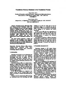
A Model of the Cholesterol Synthesis Pathway

Here we illustrate our translation workflow by using the cholesterol synthesis pathway as an example. We first draw an SBGN-PD map of this pathway (Figure 4) in the Edinburgh Pathway Editor (EPE) [46] based on the biochemical reactions listed in KEGG [27]. Then we add the necessary quantitative extensions as attributes to the corresponding glyphs in EPE (for screenshot see Figure 2), before we export the model from EPE to SBGNtext. SBGNtext is automatically translated to Bio-PEPA with the help of SBGNtext2BioPEPA [34]. Finally the model is simulated in the Bio-PEPA Eclipse Plugin Version 0.1.7 [3] using the Gibson-Bruck stochastic simulation method [19] and the Adaptive Dormant Prince ODE solver. Fluxes are computed from the exported time courses as described below. Since our model is focussed on the flux of de novo cholesterol production, we choose to ignore the complex processes that degrade or store cholesterol. Scaling of the System. Since Bio-PEPA and SBML [25] describe systems in terms of explicit molecule counts and not concentrations, we introduce a scaling factor Ω which is used to represent the size of the system. The factor Ω effectively converts a concentration [mM] into a molecular count by multiplying it with Avogadro’s number and a volume. As a volume we cannot use the typical volume of a cell, since cholesterol synthesis is confined to the endoplasmatic reticulum, which comprises only a fraction 4

Our prototypic implementation of the workflow presented here passes propensity functions entered in the Edinburgh Pathway Editor without modification to Bio-PEPA. A version of SBGNtext2BioPEPA that substitutes parameters in functions is available from [34].

15

cholesterol

acetyl-CoA

HMGCS1 DHCR7 statin

HMG-CoA desmosterol

7-dehydro-cholesterol HMGCR SC5DL mevalonate

7-dehydro-desmosterol

lathosterol MVK EBP mevalonate-5P

cholestra-7,24-dien-3beta-ol

cholestra-8,en-3beta-ol PMVK DHCR24 mevalonate-5PP

zymosterol

MVD

isopentyl-PP

4-methyl-zymosterol GGPS

EUPPS

FDPS HSD17B7

3-keto-4-methyl-zymosterol

farnesyl-PP

NSDHL

FDFT1

4-methyl-zymosterol-carboxalate

squalene

SQLE

LSS

2,3-oxydosqualene

CYP51A1

lanosterol

TM7SF2

4,4-dimethyl-cholestra-8,14,24-trienol

SC4MOL

14-demethyl-lanosterol

Fig. 4. A SBGN-PD representation of the cholesterol pathway as taken from KEGG [27], drawn in the Edinburgh Pathway Editor [46]. Metabolites are marked as yellow to highlight the mostly linear structure of the pathway. Enzymes are coloured in cyan and the inhibitory statin in red. A constant flow of acetyl-CoA is assumed to enter the system.

of the cell. At this stage we do not have information about the volume of a cell dedicated to cholesterol synthesis. However, rough estimates show that many typical enzymes that are not produced in particularly high copy numbers exist in about 104 copies / cell. Thus we choose Ω such that a 10 mM enzyme concentration translates into 10000 copies / 16

Table 4. Kinetic parameters for Michaelis-Menten reactions as used in our model. Values for the reaction rate parameters were taken from BRENDA [7] where possible. In order to have units uniformly in terms of molecule counts, KM needs to be multiplied with the system size Ω that is also used to specify the enzyme count (see as in Eq.1). Values marked with “*” are hypothetical. Reactions not listed here are assumed to follow mass action kinetics with rate constants of 1000 (reactants: 4-methyl-zymosterol, cholestra-7,24-dien-3β-ol, 7-dehydro-desmosterol) or {0.05, 50} × 10 Ω (product: acetyl-CoA).

Enzyme

Enzyme count Turnover kcat [1/h] KM [mM]

HMGCS1

10 Ω

1000

*

0.01

HMGCR

{3, 10, 30} Ω * 500

*

0.07

MVK

10 Ω

*

1000

*

PMVK

10 Ω

*

36720

0.025

MVD

10 Ω

*

17640

0.0074

EUPPS

10 Ω

*

1000

*

0.01

*

GGPS

10 Ω

*

1000

*

0.01

*

FDPS

10 Ω

*

1000

*

0.01

*

FDFT1

10 Ω

*

1908

0.0023

SQLE

1000 Ω

65.88

0.0077

*

*

0.024

LSS

10 Ω

*

1000

*

0.015

CYPY1A1

10 Ω

*

1000

*

0.005

TM7SF2

10 Ω

*

1000

*

0.0333

SC4MOL

10 Ω

*

1000

*

0.01

NSDHL

10 Ω

*

1000

*

0.007

HSD17B7

1000 Ω

DHCR24 - zymosterol

10 Ω

*

1000

*

0.037

DHCR24 - desmosterol

*

*

177.48

*

0.236

10 Ω

*

1000

0.01

*

EBP - cholestra-8,en3β-ol 10 Ω

*

5122.8

0.01

*

EBP - zymosterol

10 Ω

*

1522.8

0.05

SC5DL DHCR7

10 Ω 10 Ω

* *

1000 1000

* *

0.032 0.277

cell (Ω = 1000), giving our model a realistic scale. Explicitly representing Ω increases the flexibility of the model by allowing quick changes to the size of the system5 . Reaction Kinetics. Our typical kinetic law (propensity function for stochastic simulations; rate law for ODE) for standard Michaelis Menten kinetics as entered in EPE 5

Since parameters cannot be defined explicitly in the current EPE prototype, we model Ω as a “dummy-species”, that does not take part in reactions, but has a constant value, which can be referred to in propensity functions for the purpose of scaling KM . Since the initial “Entity Count” needs to be an integer of the right size we enter 10000 directly (= 10 · Ω).

17

is

kcat · EnzymeName Ent · m S ubstrateName Ent (1) (KM · Ω) + m S ubstrateName Ent This function is used to model all reactions that involve one enzyme and one metabolite. To do this we retrieved kinetic parameter values from BRENDA [7]. If no kinetic parameter was found for an enzyme, we assumed a turnover of kcat =1000 [1 / h] and a Michaelis-Menten constant of KM =0.01 [mM], which is of the same order of magnitude as the mean of corresponding values of other enzymes that have been observed in experiments. Table 4 reports all relevant parameters used in our model. The reaction catalysed by HMGCR has been described as a rate limiting step of the cholesterol pathway [30, 37]. To capture this notion in our model we increase the enzyme copy numbers for SQLE and HSD17B7, two slow reactions for which both kcat and KM are known. For reactions without an enzyme in Figure 4 we assumed mass action kinetics. We chose rates so that they would not be limiting in this system and would not force the accumulation of large amounts of reactants (see Table 4). The first mass action reaction is special since it determines the flux of acetyl-CoA into the system. In the absence of degradation reactions for intermediate metabolites and the endproduct cholesterol, the influx determines the rate of cholesterol production – unless intermediate metabolites accumulate (see below). We chose to model two scenarios: a low-flux scenario that represents situations where acetyl-CoA in the cell is directed away from cholesterol synthesis and a high-flux scenario that reflects conditions of more abundant acetyl-CoA. In the low and high flux scenarios 500 = 0.05 · 10 Ω and 500000 = 50 · 10 Ω molecules of acetyl-CoA are introduced into the system, respectively (10 Ω was chosen to be of the same order of magnitude as the typical number of copies per enzyme). In order to model competitive inhibition by statin we use the following kinetic law: kcat · EnzymeName Ent · m S ubstrateName Ent m S ubstrateName Ent + (KM · Ω) · (1 + m InhibitorName Ent/(Ω · KI ))

(2)

where HMGCR is the enzyme, HMG-CoA the metabolite, statin the inhibitor and KI = 0.000044 [mM] the inhibition constant average of 11 values for human cells found in BRENDA; values for other reactions are given in Table 4 . From the nature of this function it follows that any number of inhibitor molecules can be rendered ineffective, if countered by a sufficiently large number of metabolites (see results below). Measurement of Cholesterol Flux. Due to the linear structure of the pathway, its unidirectional flow and the lack of degradation of intermediate products, a steady flow of acetyl-CoA leads to a steady production of cholesterol. If the rate of an intermediate reaction is too low, the production of cholesterol is slowed down temporarily until the substrate of the reaction has accumulated enough to compensate for the reduction. A simulation in the high flux environment without statin and for HMGCR = 30000 showed that all intermediates equilibrate after less than 5 minutes and then fluctuate around fairly low molecule counts (most around zero, all below 500). To facilitate measurements of cholesterol production flux F, we omitted cholesterol degrading reactions. Instead we compute F, the flux of newly synthesised molecules of cholesterol / hour as F=

CT2 − CT1 T2 − T1 18

(3)

where C represents accumulated counts of synthesised cholesterol molecules in the system at the corresponding points T 1 and T 2 and time is measured in hours. Visual inspection of all time courses with only 1 statin molecule present indicates that the cholesterol increase follows a straight line almost immediately from the start. This is confirmed by comparisons between the fluxes measured over the first and last quarter of the first hour simulated in ODEs which differ by less than 5%, a difference that is exceeded by the stochastic noise in the low-flux system. For stochastic simulations, measuring flux over a whole hour integrates more events leading to less variance than measuring shorter intervals. Thus we report as F the number of cholesterol molecules synthesised in the first hour after starting the simulation with all metabolites at zero. Since this number varies in stochastic simulations, we report the mean and standard deviation of five simulations in this case. As discussed below, the structure of this system is such that eventually cholesterol production will always reach a level that is equivalent to the influx of acetyl-CoA, even though this may be unrealistic in a cell because HMG-CoA is degraded in some other way or produced at lower rates. Thus it is desirable to measure flux as early as possible in this system; hence we limited most of our measurements to the first hour. 6.2

Simulation Results and Biological Interpretation

Statins (or HMG-CoA reductase inhibitors) are drugs widely-used to lower cholesterol levels [8, 31, 2]. They act by inhibiting the production of mevalonate that is catalysed by HMGCR, a step widely believed to be rate limiting for cholesterol production [21]. Much previous work has investigated this step in isolation [21, 30, 37], but little is known about the quantitative dynamics of the whole pathway. Here we analyse a model that provides the opportunity to quantitatively investigate the dynamics of the whole pathway. We have chosen values for unknown parameters that reflect the intuition of many biologists that HMGCR is rate limiting. This provides an optimal starting point for exploring the potential of statin to inhibit cholesterol production. More specifically we are interested in evaluating how the function of statin is affected by natural diversity in the rate at which HMGCR catalyses the reaction that is blocked competitively by statin [30, 37]. Such diversity in rate can come from variation in the numbers of enzymes per cell (e.g. different transcription, translation and degradation rates) or from variation in the turnover of the enzyme as caused by point mutations affecting its catalytic centre. We simulated the model in two settings, one with a high flux of acetyl-CoA using ODEs and one with a low flux of acetyl-CoA using stochastic simulations, reflecting conditions when the cell directs acetyl-CoA elsewhere. For each set we chose effective numbers of HMGCR = 3000, 10000 and 30000 copies per cell to capture natural diversity. We then measured for each of these six sets (3x ODE, 3x stochastic simulations) the flux of cholesterol at 14 different statin molecule counts in the system, spanning over seven orders of magnitude. The ODE analysis in Figure 5A shows that cells with higher effective concentrations of HMGCR require larger doses of statin to shut down cholesterol synthesis. Repeating the same for a low flux of acetyl-CoA using stochastic simulations confirms this and indicates that the flux of acetyl-CoA into this pathway does not affect the relative 19

cholesterol flux [molecules / hour]

A 6x10

5

HMGCR = 3000 HMGCR = 10000 HMGCR = 30000

5x105 4x105 3x105 2x105 1x105 0

cholesterol flux [molecules / hour]

B 500.0

HMGCR = 3000 HMGCR = 10000 HMGCR = 30000

400.0 300.0 200.0 100.0 0.0 1

10

100

1000

104

105

statin molecules in the system

106

107

Fig. 5. Response of cholesterol flux to different amounts of statin molecules in the system. (A) Assuming a high influx of acetyl-CoA as computed by the Adaptive Dormant Prince ODE solver predicts mean expected values. This approximation works well for large molecule counts. (B) Assuming a low influx of acetyl-CoA as computed by the Gibson-Bruck stochastic simulator shows the variability associated with low copy numbers of molecules. Values were computed by the the Bio-PEPA Plugin 0.1.7 and report the average of five runs with error bars denoting standard deviations. We deliberately avoided averaging over many more repeats to highlight the stochastic nature of the system.

20

cholesterol flux IC50 [molec. / hour]

450

400

350

300

250

200 1

10

100

1000

10000

100000

1000000

HMGCR molecules Fig. 6. The stochastic variability of the flux of cholesterol for a wide range of enzyme copy numbers with a corresponding number of inhibitory statin molecules as given below. The higher flux for 1 and 3 HMGCR molecules is caused by rounding off fractions computed by equation (4) to get molecule counts. Error bars denote standard deviations observed in 50 stochastic runs, measuring flux in the last hour of 2h simulations, as computed by the Gibson-Bruck stochastic simulator. The number of statin molecules used in the simulations shown here for a given HMGCR count were computed by rounding the result of equation (4). This resulted in the following HMGCR → statin pairs: 1 → 0; 3 → 1; 10 → 6; 30 → 18; 100 → 62; 300 → 188; 1000 → 628; 3000 → 1885; 1 × 104 → 6285; 3 × 104 → 18857; 1 × 105 → 62857; 3 × 105 → 188571; 1 × 106 → 628571.

power of statins to shut down cholesterol production (although it does affect the absolute amount produced; see y-axes in Figure 5 for comparison). Changes appear to be linear in that 10x more HMGCR requires 10x more statin to block and a 1000x higher flux requires 1000x more statin to reduce it to the level of the low flux we observed. The slight increase in flux with some of the numbers of statin molecules in Figure 5B is not significant (see error bars). To investigate the effects of statin on the variability of flux at very low copy numbers of HMGCR we calculated the analytically expected number of statin molecules that blocks 50% of the flux of acetyl-CoA to cholesterol under a regime that leads to a local equilibrium of 500 molecules of HMG-CoA (this is similar to our low-flux regime). The expected number of inhibitor molecules I that achieves this effect is given by I = KI Ω

kcat ES − S T F − T FKM Ω T FKM Ω

(4)

where E counts the enzyme HMGCR, S counts the substrate HMG-CoA (assumed to be 500), kcat = 500 [1/h], KM =0.07 [mM], Ω=1000, T is the target flux to cholesterol assumed to be 500 [1/h], F = 50% is the fraction to which the flux should be reduced 21

cholesterol flux [molecules / hour]

1h 10h 100h

500.0

400.0

300.0

200.0

100.0

0.0 1

10

100

1000

10000

100000

1000000 10000000

statin molecules in the system Fig. 7. Statin loses its inhibitory power if enough HMG-CoA accumulates over time in the absence of other degradation routes. The error bars denote the standard deviation of five different stochastic runs, as computed by the Gibson-Bruck stochastic simulator.

by statin and KI = 0.000044 [mM] is the inhibition constant of statin. Figure 6 shows that the stochastic variability of the flux of cholesterol does not depend on the enzyme copy number although it is not possible to adjust the flux precisely for very few enzymes since the number of statin molecules has to be an integer (rounding off caused the higher flux in Figure 6). Our model also allows us to investigate acquired tolerance towards statin as caused by the structure of the pathway. Figure 7 shows a comparison of the low flux environment with HMGCR = 10000, as observed over 1 h, 10 h and 100 h (each measured flux averages only over the last hour before the end of the observation interval, where the observations start in equilibrium at 0 h with the addition of statin and end after the specified time). Assuming that HMG-CoA is not degraded by alternative pathways and all reactions are irreversible, a more than 10x higher statin concentration is needed to block cholesterol production over 10 h than when only 1 h needs to be blocked. Shutting down cholesterol production by competitive inhibition in our model leads to a continuous buildup of HMG-CoA since this metabolite is continuously produced and is not otherwise degraded. Because inhibition depends on an excess of statin in comparison to the metabolite HMG-CoA (see equation 2), given enough time the buildup of HMG-CoA will overpower any number of inhibitor molecules, making the pathway tolerant to the number of inhibiting molecules applied. This is demonstrated by the need for higher statin molecule numbers to shut down cholesterol production over longer periods of time (see Figure 7). In real cells an unbounded increase of any metabolite is not possible and might even be actively avoided by cells, thus acquired statin tolerance is limited in a natural setting. Nevertheless these findings indicate that the flexibility of 22

pathways in circumventing obstacles needs to be considered in addition to variability in HMGCR levels and acetyl-CoA flux when calculating the right dose of statins.

7

Related Work

There are various languages associated with tools that map visual diagrams to quantitative modelling environments (e.g. SPiM [40], BlenX [14], Kappa-calculus [12], Snoopy [22], EPN-PEPA [45], JDesigner [44]). However the corresponding graphical notations are not as rich as SBGN-PD and are thus not easily applied to the wide range of scenarios that SBGN-PD was designed for. Since SBGN-PD is emerging as a new standard, it is clearly desirable to translate from SBGN-PD to a quantitative environment. Since the first draft of SBGN-PD has been published in August 2008, a number of tools have been developed to support it, including the Edinburgh Pathway Editor [46], Arcadia for visualisation [47] , TinkerCell that is linked to the Systems Biology Workbench [6], and PathwayLab [26]. The graphical editor CellDesigner [18] supports a subset of SBGN-PD and can translate it into SBML which is supported by many quantitative analysis tools. However the process of adding quantitative information involves cumbersome manual interventions. This motivated work for SBMLsqueezer [16], a CellDesigner plug-in that supports the automatic construction of generalised mass action kinetics equations. While the automated suggestions for the kinetic laws from SBMLsqueezer might be of interest for some problems, the generated reactions contain many parameters that are extraordinarily difficult to estimate. Thus it is preferable to also allow the user to enter arbitrary kinetic laws that may have to be hand-crafted, but whose equations are simpler and require fewer parameter estimates. In SBGNtext2BioPEPA this is combined with mechanisms to reuse the code for such kinetic laws, greatly reducing practical difficulties and the potential for errors.

8

Conclusion and Perspectives

Since biologists are much more comfortable with drawing visual diagrams than writing code, support for translating SBGN-PD into quantitative analysis frameworks can play a key role in facilitating quantitative modelling. Our experiences with modelling the cholesterol pathway have highlighted the value of quick access to details of the model from an SBGN-PD compliant editor like Edinburgh Pathway Editor. The tool-chain described here efficiently transforms a graphical SBGN-PD model into SBGNtext, which is then compiled into a Bio-PEPA model that is ready for simulation. The simulation results presented here show that this system can indeed be used for analysing non-trivial questions. The workflow presented here critically depends on the process flow abstraction that implicitly underlies SBGN-PD. We have explicitly described this process flow abstraction and used it to design a mechanism for translating SBGN-PD into a computational model that can be used for quantitative analysis. In order to do this we build on SBGNtext, a textual representation of SBGN-PD that we created [34, 35] and that focusses on the key functional SBGN-PD content, avoiding the clutter that comes from storing graphical details. We have developed our translator SBGNtext2BioPEPA in Java 23

to facilitate its integration with the Bio-PEPA Eclipse Plugin and the Systems Biology Software Infrastructure (SBSI) that is currently under development at the Centre for Systems Biology at Edinburgh (http://csbe.bio.ed.ac.uk/). SBGNtext2BioPEPA contains a parser for SBGNtext based on a formal ANTLR EBNF grammar and is freely available [34]. Building on the process flow abstraction and the internal representation of entities, processes, arcs and parameters in our code facilitates implementing translations of SBGNtext to other modelling languages. Acknowledgements. We thank Stephen Gilmore for helpful comments that improved this manuscript. The Centre for Systems Biology Edinburgh is a Centre for Integrative Systems Biology (CISB) funded by BBSRC and EPSRC, reference BB/D019621/1.

References 1. Akman, O.E., Guerriero, M.L., Loewe, L., Troein, C.: Complementary approaches to understanding the plant circadian clock. In: Proc. of FBTC’10. EPTCS, vol. 19, pp. 1–19 (2010) 2. Baigent, C., Keech, A., Kearney, P.M., Blackwell, L., Buck, G., Pollicino, C., Kirby, A., Sourjina, T., Peto, R., Collins, R., Simes, R.: Efficacy and safety of cholesterol-lowering treatment: prospective meta-analysis of data from 90,056 participants in 14 randomised trials of statins. Lancet 366, 1267–1278 (2005) 3. Bio-PEPA homepage: http://www.biopepa.org/. To install the Bio-PEPA Eclipse Plug-in by Adam Duguid follow the links from http://homepages.inf.ed.ac.uk/jeh/Bio-PEPA/Tools.html (2009) 4. Calder, M., Duguid, A., Gilmore, S., Hillston, J.: Stronger computational modelling of signalling pathways using both continuous and discrete-state methods. In: Proc. of CMSB’06. LNCS, vol. 4210, pp. 63–77 (2006) 5. Calder, M., Hillston, J.: Process algebra modelling styles for biomolecular processes. Transactions on Computational Systems Biology XI, 1–25 (2009) 6. Chandran, D., Bergmann, F., Sauro, H.: TinkerCell: modular CAD tool for synthetic biology. Journal of Biological Engineering 3(1), 19 (2009), http://www.tinkercell.com 7. Chang, A., Scheer, M., Grote, A., Schomburg, I., Schomburg, D.: BRENDA, AMENDA and FRENDA the enzyme information system: new content and tools in 2009. Nucleic Acids Res. 37, D588–D592 (2009), http://www.brenda-enzymes.org/ 8. Chasman, D.I., Posada, D., Subrahmanyan, L., Cook, N.R., Stanton, Jr, V.P., Ridker, P.M.: Pharmacogenetic study of statin therapy and cholesterol reduction. JAMA 291, 2821–2827 (2004) 9. Ciocchetta, F., Gilmore, S., Guerriero, M.L., Hillston, J.: Integrated Simulation and ModelChecking for the Analysis of Biochemical Systems. In: Proc. of PASM’08. ENTCS, vol. 232, pp. 17–38 (2009) 10. Ciocchetta, F., Hillston, J.: Bio-PEPA: a Framework for the Modelling and Analysis of Biological Systems. Theoretical Computer Science 410(33-34), 3065–3084 (2009) 11. Cytoscape Consortium: Cytoscape Home page. http://cytoscape.org/ (2009) 12. Danos, V., Feret, J., Fontana, W., Harmer, R., Krivine, J.: Rule-based modelling of cellular signalling. In: Proc. of CONCUR’07. LNCS, vol. 4703, pp. 17–41 (2007) 13. Danos, V., Laneve, C.: Formal molecular biology. Theoretical Computer Science 325, 69– 110 (2004) 14. Dematt´e, L., Priami, C., Romanel, A.: The BlenX Language: A Tutorial. In: SFM’08, LNCS, vol. 5016, pp. 313–365 (2008)

24

15. Demir, E., Babur, O., Dogrusoz, U., Gursoy, A., Nisanci, G., Cetin-Atalay, R., Ozturk, M.: PATIKA: an integrated visual environment for collaborative construction and analysis of cellular pathways. Bioinformatics 18, 996–1003 (2002) 16. Draerger, A., Hassis, N., Supper, J., Schr¨oder, A., A., Z.: SBMLsqueezer: A CellDesigner plug-in to generate kinetic rate equations for biochemical networks. BMC Systems Biology 2, 39 (2008) 17. Duguid, A., Gilmore, S., Guerriero, M.L., Hillston, J., Loewe, L.: Design and Development of Software Tools for Bio-PEPA. In: Proc. of WSC’09. pp. 956–967. IEEE Press (2009) 18. Funahashi, A., Matsuoka, Y., Jouraku, A., Morohashi, M., Kikuchi, N., Kitano, H.: CellDesigner 3.5: A Versatile Modeling Tool for Biochemical Networks. In: Proceedings of the IEEE. vol. 96 (issue 8), pp. 1254–1265 (2008), http://www.celldesigner.org/ 19. Gibson, M.A., Bruck, J.: Efficient Exact Stochastic Simulation of Chemical Systems with Many Species and Many Channels. J. Phys. Chem. 104, 1876–1889 (2000) 20. Gillespie, D.T.: Stochastic Simulation of Chemical Kinetics. Annu. Rev. Phys. Chem. 58, 35–55 (2007) 21. Goldstein, J.L., Brown, M.S.: Regulation of the mevalonate pathway. Nature 343, 425–430 (1990) 22. Heiner, M., Richter, R., Schwarick, M., C., R.: Snoopy – A tool to design and execute graph-based formalisms. Petri Net Newsletter 74, 8–22 (2008), http://www-dssz.informatik.tu-cottbus.de/software/snoopy.html 23. Hillston, J.: A Compositional Approach to Performance Modelling. Cambridge University Press (1996) 24. Hlavacek, W., Faeder, J., Blinov, M., Posner, R., Hucka, M., Fontana, W.: Rules for modeling signal-transduction systems. Science STKE 344, re6 (2006) 25. Hucka, M., Hoops, S., Keating, S., Le Nov`ere, N., Sahle, S., Wilkinson, D.: Systems Biology Markup Language (SBML) Level 2 Version 4 Release 1. Nature Proceedings (2008), http://dx.doi.org/10.1038/npre.2008.2715.1 and http://sbml.org/Documents/Specifications 26. Jansson, A., Jirstrand, M.: Biochemical modeling with Systems Biology Graphical Notation. Drug Discovery Today (2010) 27. Kanehisa, M., Goto, S., Furumichi, M., Tanabe, M., Hirakawa, M.: KEGG for representation and analysis of molecular networks involving diseases and drugs. Nucleic Acids Res. 38, D355–D360 (2010), http://www.genome.jp/kegg/ 28. Kitano, H., Funahashi, A., Matsuoka, Y., Oda, K.: Using process diagrams for the graphical representation of biological networks. Nature Biotechnology 23, 961–966 (2005) 29. Kohn, K.W., Aladjem, M.I., Kim, S., Weinstein, J.N., Pommier, Y.: Depicting combinatorial complexity with the molecular interaction map notation. Mol Syst Biol 2, 51 (2006) 30. Krauss, R.M., Mangravite, L.M., Smith, J.D., Medina, M.W., Wang, D., Guo, X., Rieder, M.J., Simon, J.A., Hulley, S.B., Waters, D., Saad, M., Williams, P.T., Taylor, K.D., Yang, H., Nickerson, D.A., Rotter, J.I.: Variation in the 3-hydroxyl-3-methylglutaryl coenzyme a reductase gene is associated with racial differences in low-density lipoprotein cholesterol response to simvastatin treatment. Circulation 117, 1537–1544 (2008) 31. Law, M.R., Wald, N.J., Rudnicka, A.R.: Quantifying effect of statins on low density lipoprotein cholesterol, ischaemic heart disease, and stroke: systematic review and meta-analysis. BMJ 326, 1423 (2003) 32. Le Nov`ere, N., Hucka, M., Mi, H., Moodie, S., Schreiber, F., Sorokin, A., Demir, E., Wegner, K., Aladjem, M.I., Wimalaratne, S.M., Bergman, F.T., Gauges, R., Ghazal, P., Kawaji, H., Li, L., Matsuoka, Y., Villeger, A., Boyd, S.E., Calzone, L., Courtot, M., Dogrusoz, U., Freeman, T.C., Funahashi, A., Ghosh, S., Jouraku, A., Kim, S., Kolpakov, F., Luna, A., Sahle, S., Schmidt, E., Watterson, S., Wu, G., Goryanin, I., Kell, D.B., Sander, C., Sauro, H., Snoep,

25

33.

34. 35.

36.

37.

38. 39. 40.

41. 42.

43.

44.

45. 46.

47.

J.L., Kohn, K., Kitano, H.: The Systems Biology Graphical Notation. Nature Biotechnology 27, 735–41 (2009) Le Nov`ere, N., Moodie, S., Sorokin, A., Hucka, M., Schreiber, F., Demir, E., Mi, H., Matsuoka, Y., Wegner, K., Kitano, H.: Systems Biology Graphical Notation: Process Diagram Level 1. Nature Preceedings (2008), http://hdl.handle.net/10101/npre.2008.2320.1 Loewe, L.: The SBGNtext2BioPEPA homepage. http://csbe.bio.ed.ac.uk/SBGNtext2BioPEPA/index.php (2009) Loewe, L., Moodie, S., Hillston, J.: Defining a textual representation for SBGN Process Diagrams and translating it to Bio-PEPA for quantitative analysis of the MAPK signal transduction cascade. Tech. rep., School of Informatics, University of Edinburgh (2009), http://csbe.bio.ed.ac.uk/SBGNtext2BioPEPA/index.php Loewe, L., Moodie, S., Hillston, J.: Quantifying the implicit process flow abstraction in SBGN-PD diagrams with Bio-PEPA. In: Proc. of CompMod’09. EPTCS, vol. 6, pp. 93–107 (2009), http://arxiv.org/abs/0910.1410 Medina, M.W., Gao, F., Ruan, W., Rotter, J.I., Krauss, R.M.: Alternative splicing of 3hydroxy-3-methylglutaryl coenzyme A reductase is associated with plasma low-density lipoprotein cholesterol response to simvastatin. Circulation 118, 355–362 (2008) Moodie, S.L., Sorokin, A., Goryanin, I., Ghazal, P.: A Graphical Notation to Describe the Logical Interactions of Biological Pathways. J. Integr. Bioinformatics 3(2), 36 (2006) Parr, T.: The Definitive ANTLR Reference: Building Domain-Specific Languages. The Pragmatic Bookshelf, Raleigh, NC (2007), http://www.antlr.org/ Phillips, A.: A Visual Process Calculus for Biology. In: Symbolic Systems Biology: Theory and Methods. Jones and Bartlett Publishers (2010, to appear), http://research.microsoft.com/en-us/projects/spim/ Priami, C.: Stochastic π-calculus. The Computer Journal 38(7), 578–589 (1995) Ramsey, S., Orrell, D., Bolouri, H.: Dizzy: stochastic simulation of largescale genetic regulatory networks. J. Bioinf. Comp. Biol. 3(2), 415–436 (2005), http://magnet.systemsbiology.net/software/Dizzy/ Raza, S., Robertson, K.A., Lacaze, P.A., Page, D., Enright, A.J., P., G., Freeman, T.C.: A logic-based diagram of signalling pathways central to macrophage activation. BMC Syst Biol 2, 36 (2008) Sauro, H.M., Hucka, M., Finney, A., Wellock, C., Bolouri, H., Doyle, J., Kitano, H.: Next generation simulation tools: the Systems Biology Workbench and BioSPICE integration. OMICS 7(4), 355–372 (2003), For the graphical front end JDesigner see http://www.sys-bio.org/software/jdesigner.htm Shukla, A.: Mapping the Edinburgh Pathway Notation to the Performance Evaluation Process Algebra. Master’s thesis, University of Trento, Italy (2007) Sorokin, A., Paliy, K., Selkov, A., Demin, O., Dronov, S., Ghazal, P., Goryanin, I.: The Pathway Editor: A tool for managing complex biological networks. IBM J. Res. Dev. 50, 561–573 (2006), http://www.bioinformatics.ed.ac.uk/epe/. This work used the Edinburgh Pathway Editor prototype version EPE-3.0.0-alpha13 from http://epe.sourceforge.net/SourceForge/EPE.html Villeger, A.C., Pettifer, S.R., Kell, D.B.: Arcadia: a visualization tool for metabolic pathways. Bioinformatics 26(11), 1470–1471 (2010)

26