E y g. F D. 0. F. 0 D y g. (6). Here u is the voltage vector of interface. Î ..... I3=I3a+I3b. (e) Replace the virtual transmission line with its equivalent circuit, and thus the original circuit is partitioned ...... Templates for the .... E-NEWSLETTER, vol.
> REPLACE THIS LINE WITH YOUR PAPER IDENTIFICATION NUMBER (DOUBLE-CLICK HERE TO EDIT)
REPLACE THIS LINE WITH YOUR PAPER IDENTIFICATION NUMBER (DOUBLE-CLICK HERE TO EDIT) < we might comprehend the distributed numerical algorithm from the viewpoint of circuit theory and microwave network. To partition a circuit, node tearing and branch tearing are two important methods [64, 47]. This paper proposes the third way, which is called wire tearing. Tearing the circuit by wires is not a new idea, since all the subcircuits are connected by wires, but we first apply this concept into the distributed numerical algorithms [58, 59]. Wire tearing can be considered as the insertion of transmission line to connect the torn nodes [61]. The advantage of wire tearing over the branch tearing and node tearing is that it does not bring in any extra energy, because all the wires are passive [27]. As a distributed numerical algorithm, VTM is similar to overlapped Block Jacobi or Block SOR method [2, 45]. We have proved that VTM is convergent to solve arbitrarily-large SPD linear system on arbitrary number of processors [59, 62]. VTM could also be considered as a new type of algebraic domain decomposition method [55]. VTM is similar to the additive Schwarz method with Robin condition, i.e. Schwarz-Robin method [35, 21, 22, 36]. Additive Schwarz method is mainly used to solve the sparse linear system from elliptic partial differential equations (PDE), and VTM is used to solve the general sparse linear system. The partitioning method for VTM, i.e. wire tearing, is different from the traditional partitioning methods for algebraic additive Schwarz method [22, 36]. Furthermore, the preconditioning technique for VTM is more flexible than Optimized Schwarz Method [21]. This paper is organized as follows. Section 2 presents a brief introduction to the linear system of circuit. Section 3 introduces the mathematical description of transmission line. Section 4 proposes the physical background of VTM. Section 5 describes how to partition the circuit by wire tearing. Section 6 details the algorithm of VTM. Section 7 presents the convergence theory. Section 8 provides a simple example. Section 9 discusses the preconditioning techniques for VTM. Numerical experiments are shown in Section 10. We conclude this work in Section 11. In the appendix, we present a proof for the convergence theory. II. LINEAR SYSTEM OF CIRCUIT In virtue of the nodal analysis, one circuit could be described by a sparse linear system [39]. Ax = b (1) Here x represents the nodes’ voltages, and b is the current sources flowing into the nodes. A is the coefficient matrix, which might be symmetrical, or unsymmetrical, depending on the property of circuit. If the circuit contains no voltage sources but only current sources, we call it current-driven circuit. To construct the linear system of current-driven circuit, we only need to use the nodal analysis technique, and do not need the modified nodal analysis technique [39]. If there were voltage sources in the circuit, they might be equalized into current sources, according to the Norton equivalent theory [18].
2
Fig. 1. Transmission line. (A) The circuit diagram of the transmission line. (B) The equivalent circuit of the lossless transmission line.
Lemma 1: For a current-driven linear resistor network, its coefficient matrix, A, is weakly diagonally dominant, and thus symmetrical-non-negative-definite (SNND). Further, if there is at least one resistor connecting to the ground, A is strictly diagonally dominant, and thus symmetric-positive-definite (SPD). The physical insight of this lemma is that the energy of a resistor network is always non-negative. III. TRANSMISSION LINE Transmission line is an important element in electrical and microwave engineering. It is also called cable, wire or interconnect in different contexts. The circuit diagram of the transmission line is illustrated in Fig. 1. The analytical description of the lossless or ideal transmission line is the wave equation [40, 13].
∂ 2 u ( x, t ) ∂ 2 u ( x, t ) LC (2) = ∂2 x ∂ 2t Here L is the inductance per unit length, C is the capacitance per unit length. The time domain mathematical description of the lossless transmission line is called Transmission Delay Equations, as shown in (3) [40, 8, 59].
u1 (t ) + Z ⋅ i1 (t ) = u2 (t − τ ) − Z ⋅ i2 (t − τ ) u2 (t ) + Z ⋅ i2 (t ) = u1 (t − τ ) − Z ⋅ i1 (t − τ )
(3)
Here u1(t) and u2(t) represent the port voltages. i1(t) and i2(t) represent port inflow currents. t is the time variable. τ is the propagation delay. Z is the characteristic impedance, which is positive.
> REPLACE THIS LINE WITH YOUR PAPER IDENTIFICATION NUMBER (DOUBLE-CLICK HERE TO EDIT)
REPLACE THIS LINE WITH YOUR PAPER IDENTIFICATION NUMBER (DOUBLE-CLICK HERE TO EDIT) < V. WIRE TEARING To solve the sparse linear system of a circuit, originally there is no transmission line in it, but we might figure out some way to insert transmission lines into the circuit by splitting the nodes. This partitioning technique is called wire tearing. By means of wire tearing, the original circuit is turned into a distributed circuit. It is partitioned into a number of separate sub-circuits by virtual transmission line. Later, we locate each sub-circuit into one processor, and use the digital data link to imitate the behavior of the transmission line. As the result, the distributed circuit is simulated in a distributed way. According to Lemma 2, the resistor network with wires would finally go to the steady state, which is exactly the steady state of the resistor network without wires. This lemma explains the reason that VTM could always be convergent to solve the resistor network. For the sparse linear system of a general circuit, VTM might be unconvergent. There are 4 steps to perform wire tearing for the circuit G . Γ denotes the set of all the nodes in G . Step 1. Set the splitting interface Γ interface ⊆ Γ . V is called
interfacial node if V ∈ Γinterface ; otherwise, V is called inner node. Step 2. Split each interfacial node into a pair of nodes, which are called twin nodes. Step 3. Split the resistors and current sources connected to each interfacial node. Step 4. Connect each pair of twin nodes by a length of lossless wire. Add inflow currents to the twin nodes. Example 1. Fig. 4 illustrates an example, in which a simple resistor network is split into two sub-circuits.
4
First we define the set of inner nodes in Sub-circuit 1 as
Γ1,inner , the set of inner nodes in Sub-circuit 2 as Γ 2,inner . By reordering the rows, the sparse linear system of circuit (1) could be re-formatted as below by row reordering:
C F1 F2
E1 D1 0
E2 u f 0 y 1 = g1 D2 y 2 g 2
(6)
Here u is the voltage vector of Γ interface . y1 and y2 are the voltage vector of
Γ1,inner and Γ 2,inner , respectively.
After wire tearing, the interfacial nodes are split, and
Γinterface is split into two sets, the twin nodes in Sub-circuit 1, Γ1,twin , and the twin nodes in Sub-circuit 2, Γ 2,twin . The system of sub-circuit 1 is:
C1 F 1
E1 u1 f1 i1 (7) = + D1 y 1 g1 0 u1 represents the voltage vector of Γ1,twin . i1 represents the currents flowing into
Γ1,twin .
After wire tearing, the system of sub-circuit 2 is:
C 2 F 2
E 2 u 2 f 2 i 2 = + D2 y 2 g 2 0
(8)
Here u 2 represents the voltages vector of
Γ 2,twin . i 2
represents the currents flowing into each node of
Γ 2,twin .
Also we have,
Fig. 4. Illustration of the wire tearing. (a) The original resistor network, and node 2 is set to be the interfacial node. (b) Split node 2 into a pair of twin nodes 2a and 2b, and insert a length of transmission line between them. 1/R2=1/R2a+1/R2b. I2=I2a+I2b. (c) Replace the virtual transmission line with its equivalent circuit, and the original resistor network is partitioned into two sub-networks.
> REPLACE THIS LINE WITH YOUR PAPER IDENTIFICATION NUMBER (DOUBLE-CLICK HERE TO EDIT)
REPLACE THIS LINE WITH YOUR PAPER IDENTIFICATION NUMBER (DOUBLE-CLICK HERE TO EDIT)
0 . I is the identity matrix.
2.
W = diag ( C1 ) or diag ( C2 ) . We call it diagonal
g13 0
0
g3
0
g34
0 u3 g 4 u4
Here we set:
g1 = g 2 = g3 = g 4 = 1 g13 = g34 = g 42 = − g 21 = 10 The loop gain of this circuit is:
Gain = g13 g34 g 42 g 21 g1−1 g3−1 g 4−1 g 2−1 = −104 Then we partition this linear system by wire tearing,
preconditioner. 3.
W = C1 or C2 . This is called overlapped block preconditioner. It is similar to the overlapped block Jacobi method.
4.
I3 I4
W = α ⋅ C1 or α ⋅ C2 , α > 0 . This is called weighted overlapped block preconditioner (WOB). As the result, we obtain 2 sub-systems:
> REPLACE THIS LINE WITH YOUR PAPER IDENTIFICATION NUMBER (DOUBLE-CLICK HERE TO EDIT)
REPLACE THIS LINE WITH YOUR PAPER IDENTIFICATION NUMBER (DOUBLE-CLICK HERE TO EDIT)
REPLACE THIS LINE WITH YOUR PAPER IDENTIFICATION NUMBER (DOUBLE-CLICK HERE TO EDIT) < of OBJ and VTM_OB are same. For the unsymmetrical linear systems, VTM might be unconvergent. At last, we test VTM on a various number of processors, as shown in Fig. 7. In this case, we use Grid3d as the testbench. The test result indicates that the convergence speed of VTM is slightly relative to the number of processors.
9
If the delays of virtual transmission lines are different and stochastic, VTM would turn to be a fully asynchronous and chaotic numerical algorithm [58]. If we replace each variable by a piece of waveform, VTM would become a waveform-relaxation algorithm [60]. To simulate the post-layout integrated circuit in parallel, we have figured out another method to distributedly solve the nonlinear delay differential equations extracted from the distributed circuits [61]. APPENDIX Here we prove that, if the graph of the resistor network is 2-partete, VTM converges. Lemma 3: Assume a linear resistor network is partitioned into 2 sub-circuits by level-one wire tearing, if the characteristic impedance matrix Z of the virtual transmission lines is SPD, VTM converges at the answer to the resistor network. Proof:
Fig. 7. Test VTM on a number of processors.
First, we consider the resistor network with inner nodes, and eliminate these inner nodes by Schur complement technique. Then, we prove Lemma 3 for the resistor network without inner nodes. The sparse linear system of the resistor network is:
C F1 F2
XI. CONCLUSION AND FUTURE WORK In this paper, we introduce VTM to solve the sparse linear system of circuit in parallel. VTM is a distributed and stationary iterative numerical algorithm, and it is efficient to solve the resistor networks. VTM proves many insightful conclusions linking numerics and electrics. The physical background of VTM is electric circuit, and this makes this algorithm different from the traditional numerical algorithms. As presented in this paper, we have borrowed many concepts from circuit theory to describe this algorithm. According to the simple example presented in Section 9, we conclude that there exists similarity between the stability of VTM and the stability of distributed linear circuit (or microwave network). The convergence speed of VTM is highly depending on the characteristic admittance matrix of the virtual transmission lines, i.e. its preconditioner W. A number of preconditioning techniques are implemented to accelerate VTM. Experiments indicate that, if W is properly chosen, the performance of VTM would be appreciable; if not, VTM would be plain. Nevertheless, the computation cost to design the preconditioner W should be aware of [5]. For the SPD linear system, we have proved that VTM is convergent; for the large unsymmetrical linear system, we have not yet figure out an effective way to choose the characteristic admittance matrix to guarantee convergence. This is an open problem. VTM could also be used to solve the nonlinear system, as we pointed out in [59]. However, the convergence analysis of nonlinear system is more complicated than the linear system. This problem should be further studied.
E1 D1 0
E2 u f 0 y 1 = g1 D2 y 2 g 2
Eliminate the inner variables y1 and y2, we obtain:
(C - E D 1
F - E2 D-12 F2 ) u
-1 1 1
= f - E1 D1-1g1 - E2 D-12 g 2 y1 = -D1-1F1u + D1-1g1 y 2 = -D-12 F2u + D-12 g 2 Set,
S = C - E1D1-1F1 - E 2 D-12 F2 ,
r = f - E1D1-1g1 - E2 D-12 g 2 , then,
(22) S ⋅u = r S is called the Schur complement matrix associated with the interface variables u.
C E is SPD, then the Schur F D −1 complement matrix S = C - ED F is SPD. Lemma 4: If A =
If the circuit is split into two sub-circuits by level-one wire tearing, the system of Sub-circuit 1 is (7):
C1 F 1
E1 u1 f1 i1 = + D1 y 1 g1 0
Eliminate the inner variables y1:
> REPLACE THIS LINE WITH YOUR PAPER IDENTIFICATION NUMBER (DOUBLE-CLICK HERE TO EDIT)
REPLACE THIS LINE WITH YOUR PAPER IDENTIFICATION NUMBER (DOUBLE-CLICK HERE TO EDIT)
0, i = 1,2, , n . Then, Assume
(Z) = Z ⋅ QTQ ⋅ ( Z ) = ( Z Q) ⋅ T ⋅ ( Z Q) T
T -1
T
Z⋅S = Z ⋅ Z ⋅S ⋅ Z ⋅ T
T
-1
T
Similarly, we obtain,
λi > 0 , i = 1, , n ,
) (
T
Z Q1
)
-1
.
T
Z ⋅ S 2 ⋅ Z = Q 2 Λ 2Q 2 T where Λ 2 = diag ( μ1 , μ 2 , , μ n ) , μi > 0 , i = 1, , n ,
Q 2Q 2 T = I . Z ⋅ S 2 =
(
T
) (
Z Q2 Λ 2
Then, (31) could be decomposed as below:
T
-1
T
1
1
1
-1
T
−1
1
1
1
T
−1
= Z −1
Z Q1 Λ 1
T
T
= Z −1
T
(
1
1
T
1
-1
T
−1
1
1
1
1
n
1
n
T
-1
1
Z
−1
Z ⋅ S1 ⋅ Z = Q1 Λ1Q1T
Q1Q1T = I . Z ⋅ S1 =
1
T2 = Z −1 ( I − Z ⋅ S 2 )( I + Z ⋅ S 2 ) Z
According to Lemma 5 and 6, we come to know that,
T
-1
T
1
Similarly, (32) could be decomposed as:
End of proof.
where Λ1 = diag (λ1 , λ2 , , λn ) ,
−1
1
T
−1
-1
−1
T
1
−1
T -1
T
11
Z Q2
)
-1
.
( (
) ( )Z 1− μ 1− μ , , Z Q ) ⋅ diag ⋅ Z Q ) 1+ μ ( 1+ μ T
Z Q 2 ( I − Λ 2 )( I + Λ 2 ) T
2
−1
T
Z Q2
1
n
1
n
-1
T
2
The spectral radius of T1T2 is defined as:
ρ (T1T2 ) = lim ( T1T2 )
k 1/ k
k →∞
So we first calculate
( T1T2 )
norm of the square matrix A.
k
. Here A is the spectral
-1
Z
> REPLACE THIS LINE WITH YOUR PAPER IDENTIFICATION NUMBER (DOUBLE-CLICK HERE TO EDIT)
0 , i = 1, , n ,
( W − S2 ) −1 × ( W + S 2 ) ( W − S1 ) u1k − 2 −1 −1 + ( W + S1 ) ( W − S 2 ) ( W + S 2 ) r −1 +( W + S1 ) r
k
−1
−1
−1 −1 u1∞ = I − ( W + S1 ) ( W − S 2 )( W + S 2 ) ( W − S1 ) −1 −1 −1 × ( W + S1 ) + ( W + S1 ) ( W − S 2 ) ( W + S 2 ) ⋅ r
= ( W + S1 ) − ( W − S 2 )( W + S 2 )
−1
( W − S1 )
−1
−1 × I + ( W − S 2 ) ( W + S 2 ) ⋅ r
( (
) )
(
)
−1
−1
I + W − S W + S −1 −1 ( 2 )( 2) = r −1 × I − ( W − S 2 )( W + S 2 ) W + S1
(
)
−1
( W + S ) ( ( W + S ) + ( W − S ) )−1 2 2 2 r = × ( ( W + S ) − ( W − S ) ) ( W + S )−1 W + S 2 2 2 1 = ( W + S 2 )( 2 W )
k →∞
1 − λ1 1 − λn ≤ max , , 1 + λn 1 + λ1 1 − μ1 1 − μn , , × max 1 + μn 1 + μ1 = ρ (T1 ) ρ (T2 ) Because λi > 0 , i = 1, , n ,
So we conclude that VTM converges for 2-partite resistor network [45]. According to (27), when this algorithm is convergent,
I − ( W − S )( W + S )−1 W + 2 2 = −1 I + ( W − S 2 )( W + S 2 ) S1 −1 × I + ( W − S 2 ) ( W + S 2 ) ⋅ r
k
1 − μ1 1 − μn × diag , , ⋅ 1 + μn 1 + μ1
ρ (T1T2 ) < 1
Z
Q ⋅ ( I − Λ )( I + Λ )−1 ⋅ Q T 1 1 1 1 ⋅ −1 T × Q 2 ⋅ ( I − Λ 2 )( I + Λ 2 ) ⋅ Q 2
( I − Λ )( I + Λ )−1 ⋅ 1 1 ⋅ −1 × ( I − Λ 2 )( I + Λ 2 )
Consequently,
u1k = ( W + S1 ) ⋅
×Q 2 ( I − Λ 2 )( I + Λ 2 ) Q T2
k
< 1 .
ρ (T2 ) = max
u1k = u1k − 2 = u1∞ , then,
Z k
−1
⋅
)
k
−1
=
1 − μ1 1 − μn , , 1 + μn 1 + μ1
k
12
−1
( 2S 2 )( W + S 2 )
−1
−1
W + S1 r −1
−1 = ( W + S 2 ) W −1S 2 ( W + S 2 ) W + S1 r −1
−1 = ( I + S 2 W −1 ) S 2 ( I + W −1S 2 ) + S1 r −1
−1 = ( S 2 + S 2 W −1S 2 )( I + W −1S 2 ) + S1 r −1
−1 = S 2 ( I + W −1S 2 )( I + W −1S 2 ) + S1 r
< 1 ;
= [ S 2 + S1 ] r −1
= S −1 ⋅ r Until now, we have proved that, VTM is convergent for 2-partite resistor network when using level-one wire tearing.
> REPLACE THIS LINE WITH YOUR PAPER IDENTIFICATION NUMBER (DOUBLE-CLICK HERE TO EDIT) < For the more general cases, the resistor network is k-partite, and the wire tearing might be level-one or multilevel. A general proof was presented in [62]. ACKNOWLEDGMENT Discussions with Hao Zhang, Yi Su, Bin Niu, Yu Wang, Wei Xue, Peng Zhang and Chun Xia were very helpful. Thanks are due to Qi Wei, Bo Zhao, Xia Wei, Xiaojian Mao, Yongpan Liu, Fei Qiao and Rong Luo for encouragement and support. We are very grateful for the public domain softwares provided by John R. Gilbert, Tim A. Davis, Robert Bridson, Haifeng Qian and et al.
[17]
[18] [19]
[20]
[21]
REFERENCES [1]
[2]
[3]
[4]
[5] [6]
[7]
[8] [9] [10]
[11]
[12]
[13] [14]
[15]
[16]
S. Balay, K. Buschelman, V. Eijkhout, W. D. Gropp, D. Kaushik, M. G. Knepley, L. Curfman McInnes, B. F. Smith and H. Zhang, PETSc Users Manual, ANL-95/11 - Revision 2.1.5, Argonne National Laboratory. R. Barrett, M. Berry, T. Chan, J. Demmel, J. Donato, J. Dongarra, V. Eijkhout, R. Pozo, C. Romine and H. Van der Vorst. Templates for the solution of Linear Systems: Building Blocks for Iterative Methods, 2nd Edition, SIAM, 1994. A. Basermann, U. Jaekel, and K. Hachiy. Preconditioning parallel sparse iterative solvers for circuit simulation. In Proceedings of the 8th SIAM Proceedings on Applied Linear Algebra, Williamsburg VA, 2003. A. Basermann, U. Jaekel, and M. Nordhausen. Parallel iterative solvers for sparse linear systems in circuit simulation. Fut. Gen. Fut. Gen.. Comput. Sys., 21(8):1275–1284, 2005. M. Benzi. Preconditioning techniques for large linear systems: A survey. Journal of Computational Physics, 182:418–477, 2002. J. Bolz, I. Farmer, E. Grinspun, and P. Schröoder. Sparse matrix solvers on the GPU: conjugate gradients and multigrid. In ACM SIGGRAPH 2003 (San Diego, California, July 27 - 31, 2003). C. W. Bomhof and H. A. Van der Vorst, A parallel linear system solver for circuit simulation problems, Numerical Linear Algebra with Applications, 7 (2000). F. H. Branin. Transient analysis of lossless transmission lines, Proceedings of the IEEE, vol. 55, pp. 2012–2013, Nov. 1967. R. Bridson. A MATLAB CMEX interface to the Metis library. Available at http://www.stanford.edu/~rbridson/download/metismex.c R. Bridson and W.-P. Tang. Refining an approximate inverse. Journal on Computational and Applied Math, 123 (2000), Numerical Analysis 2000 vol. III: Linear Algebra, pp. 293-306. S. Cauley, V. Balakrishnan, Cheng-Kok Koh, A parallel direct solver for the simulation of large-scale power/ground networks, IEEE Transactions on Computer-Aided Design of Integrated Circuits and Systems, v.29 n.4, p.636-641, April 2010. T. H. Chen and C. C.-P Chen. Efficient large-scale power grid analysis based on preconditioned Krylov-subspace iterative methods. In Proc. IEEE/ACM DAC, pages 559--562, 2001. R. E. Collin. Foundations for microwave engineering, 2nd edition, Wiley-IEEE Press, 2000. T. A. Davis and Y. F. Hu. The University of Florida Sparse Matrix Collection. Submitted to ACM Transactions on Mathematical Software. Available at: http://www.cise.ufl.edu/research/sparse/matrices/ J. Demmel, J. Gilbert, and X. Li. An asynchronous parallel supernodal algorithm for sparse gaussian elimination. SIAM J. Matrix Analysis and Applications, 20(4): 915–952, 1999. Zhuo Feng, Peng Li. Multigrid on GPU: tackling power grid analysis on parallel SIMT platforms, Proceedings of the 2008 IEEE/ACM
[22] [23] [24]
[25] [26]
[27]
[28]
[29]
[30] [31]
[32]
[33] [34] [35]
[36]
13
International Conference on Computer-Aided Design, November 10-13, 2008, San Jose, California. Zhuo Feng, Zhiyu Zeng. Parallel multigrid preconditioning on graphics processing units (GPUs) for robust power grid analysis. In Proceedings of the 47th Design Automation Conference (Anaheim, California, June 13 18, 2010). DAC '10. ACM, New York, NY, 661-666. T. L. Floyd. Principles of electric circuits, 6th edition, Prentice Hall, 1999. David Fritzsche, Andreas Frommer, and Daniel B. Szyld, Overlapping blocks by growing a partition with applications to preconditioning, Research Report 10-07-26, Department of Mathematics, Temple University, July 2010. N. Frohlich, B. M. Riess, U. A. Wever, and Q. Zheng A New Approach for Parallel Simulation of VLSI Circuits on a Transsitor Level. TCAD, June 1998. M. J. Gander, L. Halpern, and F. Nataf. Optimized Schwarz Methods. In T. Chan, T. Kako, H. Kawarada, O. Pironneau (eds.), Proceedings of the Twelveth International Conference on Domain Decomposition, DDM press, 2001, pp. 15–27. M. J. Gander, Schwarz Methods in the Course of Time, Electronic Transactions on Numerical Analysis, 31:228–255, 2008. A. George and J. W. Liu. Computer Solution of Large Sparse Positive Definite Systems. Prentice-Hall, Englewood Cliffs, New Jersey, 1981. John R. Gilbert, Gary L. Miller, and Shang-Hua Teng. Geometric mesh partitioning: Implementation and experiments. SIAM J. Scientific Computing 19:2091-2110, 1998. G. H. Golub and C. F. Van Loan, Matrix computations. Johns Hopkins University Press, 1989. Wei Huang. HotSpot: A chip and package compact thermal modeling methodology for VLSI design. Ph.D. Dissertation, University of Virginia, 2007. Russell Kao. Piecewise Linear Models for Switch-Level Simulation. Chapter 5.6.1, Node and Branch Tearing. Technical Report, CSL-TR-92-532, Stanford University, 1992. G. Karypis and V. Kumar. Metis 4.0: Unstructured graph partitioning and sparse matrix ordering system, Technical report, Department of Computer Science, University of Minnesota, 1998. Available at http://www.cs.umn.edu/metis D. P. Koester. Parallel Block-Diagonal-Bordered Sparse Linear Solvers for Power Systems Applications. Ph.D dissertation, Syracuse University. 1995. J. N. Kozhaya and S. R. Nassif. Fast Power Grid Simulation. In Proceedings of the 37th Design Automation Conference, 2000. J. N. Kozhaya, S. R. Nassif, and F. N. Najm, A multigrid-like technique for power grid analysis, IEEE Trans. Computer-aided Design, vol. 21, pp. 1148--1160, Oct. 2002. Zhao Li, C.-J. Richard Shi. A coupled iterative/direct method for efficient time-domain simulation of nonlinear circuits with power/ground networks. ISCAS (5) 2004: 165-168. Xiaoye S. Li. An overview of SuperLU: Algorithms, implementation, and user interface. ACM Trans. Math. Softw. 2005. Peng Li. What Is Parallel Circuit Simulation? ACM/SIGDA E-NEWSLETTER, vol. 40, No. 4, April 1, 2010 P. L. Lions, On the Schwarz alternating method III: a variant for nonoverlapping subdomains, Third International Symposium on Domain Decomposition Methods for Partial Differential Equations, 1989, Houston, Texas. Sébastien Loisel and Daniel B. Szyld, On the convergence of Optimized Schwarz Methods by way of Matrix Analysis , Domain Decomposition Methods in Science and Engineering XVIII, Michel Bercovier, Martin Gander, Ralf Kornhuber, and Olof B. Widlund, editors. Lecture Notes in Computational Science and Engineering, Vol. 70, Springer, 2009, pages 363-370.
> REPLACE THIS LINE WITH YOUR PAPER IDENTIFICATION NUMBER (DOUBLE-CLICK HERE TO EDIT) < [37] J. D. Meindl. Beyond Moore's Law: The Interconnect Era. Computing in Science and Engineering. 2003. [38] L. Nagel. SPICE2: A Computer Program to Simulate Semiconductor Circuits, Electronics Research Laboratory Report No. ERL-M520. University of California, Berkeley, 1975. [39] Jan Ogrodzki. Circuit simulation methods and algorithms. CRC Press, 1994. [40] H. J. Pain. The physics of vibrations and waves, Wiley, 1976. [41] He Peng, Chung-Kuan Cheng. Parallel transistor level full-chip circuit simulation. DATE 2009: 304-307. [42] H. Qian, S. R. Nassif, and S. S. Sapatnekar, Power grid analysis using random walks, IEEE Trans. Computer-aided Design, vol. 24, pp. 1204--1224, Aug. 2005. [43] H. Qian and S. S. Sapatnekar, Stochastic Preconditioning for Diagonally Dominant Matrices, SIAM Journal on Scientific Computing, Vol. 30, No. 3, pp. 1178 – 1204, March, 2008. [44] T. L. Quarles. Analysis of Performance and Convergence Issues for Circuit Simulation. ERL Memo No. UCB/ERL M89/42 April 1989. [45] Y. Saad. Iterative Methods for Sparse Linear Systems. The PWS Publishing Company, Boston, 1996. Second edition, SIAM, Philadelphia, 2003. [46] R. A. Saleh, K. A. Gallivan, M. C. Chang, et al. Parallel circuit simulation on supercomputers. Proceedings of the IEEE, 1989. [47] Alberto Sangiovanni-Vincentelli, Li-Kuan Chen, and Leon O. Chua. A new tearing approach – node-tearing nodal analysis. In IEEE International Symposium on Circuits and Systems, 1977. [48] Jin Shi, Yici Cai, Wenting Hou, Liwei Ma, Sheldon X.-D. Tan, Pei-Hsin Ho, Xiaoyi Wang. GPU friendly fast Poisson solver for structured power grid network analysis, Proceedings of the 46th Annual Design Automation Conference, July 26-31, 2009, San Francisco, California. [49] Ken Stanley, T. A. Davis. KLU: a "Clark Kent" sparse LU factorization algorithm for circuit matrices. 2004 SIAM Conference on Parallel Processing for Scientific Computing (PP04). Originally appeared in NA Digest, 1997. [50] Heidi K. Thornquist, Eric R. Keiter, Robert J. Hoekstra, David M. Day, Erik G. Boman, A parallel preconditioning strategy for efficient transistor-level circuit simulation, Proceedings of the 2009 International Conference on Computer-Aided Design, November 02-05, 2009, San Jose, California. [51] John R. Gilbert. Meshpart, a public domain matlab toolbox for sparse matrix partitioning. Available at http://www.cerfacs.fr/algor/Softs/MESHPART/ [52] CircuitSim90, 1990 Circuit Simulation and Modeling Workshop at MCNC, Available at http://www.cbl.ncsu.edu/CBL_Docs/csim90.html [53] Mathworks Corparation. Matlab User Manual. R13. 2002. [54] Mathworks Corparation. Simulink User Manual. R13. 2002. [55] A. Toselli and O. Widlund. Domain Decomposition Methods – Algorithms and Theory. Springer Series in Computational, Mathematics 34, Springer, Berlin, Heidelberg, 2005. [56] R. S. Varga. Matrix Iterative Analysis. Prentice-Hall, Englewood Cliffs, New Jersey, 1962. Second Edition, Springer Series in Computational Mathematics 27, Springer, Berlin, Heidelberg, New York, 2000. [57] W. T. Weeks, A. J. Jimenez, G. W. Mahoney, and D. Mehta. Algorithms for ASTAP - A Network-Analysis Program. IEEE Trans.Circuit Theory, CT-20(4):628-634, 1973. [58] Fei Wei, Huazhong Yang. Directed Transmission Method, A Fully Asynchronous Approach to Solve Sparse Linear Systems in Parallel. In ACM Proceedings of the 20th Symposium on Parallelism in Algorithms and Architectures (Munich, Germany, June 14 - 16, 2008). SPAA 2008. [59] Fei Wei, Huazhong Yang, Virtual Transmission Method, A New Distributed Algorithm to Solve Sparse Linear Systems. The Fourth International Conference on Networked Computing and Advanced Information Management, vol. 1, pp.703-709, 2008.
14
[60] Fei Wei, Huazhong Yang. Waveform Transmission Method, A New Waveform Relaxation Based Algorithm to Solve Ordinary Differential Equations. Preprinted. 2009. [61] Fei Wei, Huazhong Yang. Transmission Line Inspires a New Distributed Algorithm to Solve the Nonlinear Dynamical System of Physical Circuits. The 5th International Conference on Computer Sciences and Convergence Information Technology, Nov. 30, Seoul, Korea, 2010. [62] Fei Wei, Huazhong Yang. Virtual Transmission Method, Algorithm and Theory. Preprinted. 2009. [63] J. White, A. Sangiovanni-Vincentelli, Relaxation Techniques for the simulation of VLSI circuits. Kluwer Academic Publishers, 1986. [64] Felix F. Wu. Solution of large-scale networks by tearing. IEEE Transactions on Circuits and Systems, 1976. [65] Wei Xue, Jiwu Shu, Yongwei Wu, Weimin Zheng. Parallel Algorithm and Implementation for Realtime Dynamical Simulation of Power System. ICPP 2005: 137-144. [66] D. M. Young. Iterative Solution of Large Linear Systems. Academic Press, New York, 1971. [67] Yu Zhong, M. D. F. Wong, Fast algorithms for IR drop analysis in large power grid, Proceedings of the 2005 IEEE/ACM International conference on Computer-aided design, p.351-357, November 06-10, 2005. [68] Quming Zhou, Kai Sun, Kartik Mohanram, Danny C. Sorensen. Large power grid analysis using domain decomposition, Proceedings of the conference on Design, automation and test in Europe: Proceedings, March 06-10, 2006, Munich, Germany. [69] C. Zhuo, J. Hu, M. Zhao, and K. Chen. Power grid analysis and optimization using algebraic multigrid. IEEE Transactions on Computer-aided Design, 27:738–751, April 2008. Fei Wei received the B.S. degree in electronic engineering from Tsinghua University, Beijing, China in 2004. He is currently a Ph.D student in Department of Electronic Engineering, Tsinghua University. His research interests are distributed numerical algorithms and transistor-level circuit simulation. Huazhong Yang (M’97–SM’00) received the B.S. degree in microelectronics and the M.S. and Ph.D. degrees in circuits and systems from Tsinghua University, Beijing, China, in 1989, 1993, and 1998, respectively. Since 1993, he has been with the Department of Electronic Engineering, Tsinghua University, where he has been a Full Professor since 1998. His research interests include CMOS radio-frequency integrated circuits, VLSI system structure for digital communications and media processing, low-voltage and low power integrated circuits, and computer-aided design methodologies for system integration. He has authored or coauthored 6 books and more than 180 journal and conference papers in this area and holds 9 China patents. He is also a coeditor of the research monograph High-speed Optical Transceivers-Integrated Circuits Designs and Optical Devices Techniques (World Scientific, 2006). Dr. Yang was a recipient of the fund for Distinguished Young Scholars from NSFC in 2000, the outstanding researcher award of the National Keystone Basic Research Program of China in 2004, and the Special Government Allowance from the State Council of China in 2006.served as a TPC member of the Asia-Pacific Conference on Circuits and Systems, the International Conference on Communications, Circuits and Systems, and the Asia and South Pacific Design Automation Conference. He is an Associate Editor of the International Journal of Electronics.