Transverse wave propagation in a one-dimensional structure ... - Hal

Transverse wave propagation in a one-dimensional structure coupled to its electrical analogue: comparison of transfer matrix models Boris Lossouarn, Mathieu Aucejo, Jean-François Deü

To cite this version: Boris Lossouarn, Mathieu Aucejo, Jean-François Deü. Transverse wave propagation in a onedimensional structure coupled to its electrical analogue: comparison of transfer matrix models. 7th European Congress on Computational Methods in Applied Sciences and Engineering, ECCOMAS 2016, Jun 2016, Hersonissos, Greece.

HAL Id: hal-01739657 https://hal.archives-ouvertes.fr/hal-01739657 Submitted on 21 Mar 2018

HAL is a multi-disciplinary open access archive for the deposit and dissemination of scientific research documents, whether they are published or not. The documents may come from teaching and research institutions in France or abroad, or from public or private research centers.

L’archive ouverte pluridisciplinaire HAL, est destinée au dépôt et à la diffusion de documents scientifiques de niveau recherche, publiés ou non, émanant des établissements d’enseignement et de recherche français ou étrangers, des laboratoires publics ou privés.

ECCOMAS Congress 2016 VII European Congress on Computational Methods in Applied Sciences and Engineering M. Papadrakakis, V. Papadopoulos, G. Stefanou, V. Plevris (eds.) Crete Island, Greece, 5–10 June 2016

TRANSVERSE WAVE PROPAGATION IN A ONE-DIMENSIONAL STRUCTURE COUPLED TO ITS ELECTRICAL ANALOGUE: COMPARISON OF TRANSFER MATRIX MODELS B. Lossouarn1 , M. Aucejo1 , J.-F. Deu¨ 1 1 Structural

Mechanics and Coupled Systems laboratory, Conservatoire National des Arts et M´etiers 2 rue Cont´e, Paris, France e-mail: {boris.lossouarn,mathieu.aucejo,jean-francois.deu}@cnam.fr

Keywords: Wave Propagation, Transfer Matrix, Piezoelectric Coupling, Electrical Network. Abstract. Wave propagation in mechanical structures can be controlled by a coupling to an electrical network exhibiting a similar dispersion relation. The energy transfer between the two media is maximized on a broad frequency range when choosing a network that is the electrical analogue of the structure to control. In terms of structural vibration, this strategy is equivalent to a multimodal tuned mass damping. Indeed, the control is implemented thanks to a multimodal electrical network, whose modes are close enough to those of the mechanical structure. The electromechanical coupling can be achieved by using an array of piezoelectric patches, which are small enough compared to the smallest wavelength to control. Then, when considering interconnected patches, wave propagation occurs simultaneously in the mechanical and electrical media. Wave propagation in one-dimensional periodic structures can be analyzed with the transfer matrix method. In this paper, the definition of an electromechanical unit cell gives a relation between state vectors involving both mechanical and electrical degrees of freedom. As an extension of a previous work focusing on longitudinal propagation, four transfer matrix models are defined in order to describe the piezoelectric coupling of a beam to its discrete electrical analogue. Indeed, the beam can be approximated either by its discrete equivalent, a fully homogenized model, a piecewise homogenized model or a finite element model. Offering an increasing complexity, those formulations are compared in order to determine their respective limits. Depending on the frequency range of interest, it then becomes possible to choose a suitable model for the analysis of structures involving a piezoelectric coupling to their electrical analogues.

B. Lossouarn, M. Aucejo, J.-F. De¨u

1

INTRODUCTION

Multimodal vibration control can be implemented by coupling a mechanical structure to its electrical analogue. A practical solution is to cover the structure to control with an array of piezoelectric patches that are interconnected with a suitable electrical network. From a finite difference method applied to the continuous equations describing the mechanical medium, an electromechnical analogy provides the suitable electrical topology [1, 2]. This method was applied to the control of a beam and it led to a passive electrical network made of inductors and transformers [3, 4]. A periodic layout of the electromechanical structure allows using the transfer matrix method [5, 6]. This method has often been implemented in problems involving independent piezoelectric shunts [7, 8, 9] but rarely with an interconnection of successive patches [10]. This last case requires the definition of state vectors that combine both mechanical and electrical degrees of freedom, because a real electromechanical waveguide is considered. The electrical part is described with the discrete equations governing the lumped electrical components but the continuous mechanical medium can be approximated by various models. The present contribution extends previous models and results that were initially dedicated to the analysis of longitudinal wave propagation in coupled analogous waveguides [11]. When considering transverse propagation, the transfer matrices are obviously different, but the methods remain the same. A first section presents the electromechanical unit cell including a beam segment and a portion of the analogous electrical network, which was presented in [4]. Then, a model describing a pair of piezoelectric patches subjected to bending motion is proposed. In a second section, we recall the transfer matrices that were obtained in [4] when considering either a discrete or a fully homogenized beam coupled to the discrete electrical analogue. Two new models are added: a piecewise homogenized model and a finite element model, which both take into account the mechanical discontinuity induced by the addition of piezoelectric patches. The last section compares the propagation constants and the frequency response functions obtained with the four transfer matrix models, which offer an increasing complexity. The main objective is to define their respective limits and to select the most appropriate depending on the frequency range of interest and the required accuracy. 2

ANALOGOUS PIEZOELECTRIC NETWORK ON BEAM

A beam is coupled to its analogous electrical network through a periodic array of piezoelectric patches. A unit cell is defined by considering both mechanical and electrical propagation media. Then, the linear piezoelectricity theory gives a model describing a pair of piezoelectric patches subjected to bending motion. 2.1

Electromechanical unit cell

A periodic array of piezoelectric patches is distributed on an homogeneous beam. An electrical network interconnects the patches, which creates an electrical waveguide. The chosen network is the periodic electrical analogue of a beam [3, 4] because it was shown that this solution can lead to a broadband control of transverse waves. As seen in Fig. 1, an electromechanical periodic structure is obtained, so that a unit cell of length a can be defined. The thickness of the main structure is hs and its width is b. The piezoelectric patches have a thickness hp , a width b and a length lp , with lp ≤ a. Then, q˙I is the current flowing from the network to the pair of patches and VI is the voltage on the electrodes connected to the network. The two piezoelectric patches need to be transversely polarized in identical directions in order to generate a non-zero voltage when bending excitation occurs [12].

B. Lossouarn, M. Aucejo, J.-F. De¨u

L

b

L

L

L

..1 aˆ

..1

L

..

1 a ˆ/2

..

1 a ˆ/2

VI q˙I

..1

aˆ

hp

aˆ

hs

lp b

a

Figure 1: Beam segment coupled to its analogous electrical network through a periodic array of piezoelectric patches and corresponding electromechanical unit cell.

2.2

Bending model for a pair of thin piezoelectric patches

For a thin piezoelectric patch under plane-stress assumption and polarized in transverse direction [13], the 3D linear piezoelectricity theory is simplified into the one-dimensional formulation σp = YpE εp − e¯31 Ep , Dp = e¯31 εp + ¯ε33 Ep

where YpE =

1 , sE 11

e¯31 =

d31 , sE 11

and ¯ε33 = σ33 −

d231 . sE 11

(1)

εp and σp are respectively the strain and stress in the axial direction ’1’ of the piezoelectric patch. Dp and Ep are the electric displacement and electric field in the transverse direction ’3’. sE 11 is the elastic compliance at constant electric field, d31 is the piezoelectric charge constant and σ33 is the permittivity at constant stress. If we consider that the stress is constant along the thickness, the normal force Np is obtained by multiplying σp by the patch cross-section area Sp = bhp . For a thin piezoelectric patch, the electric field Ep can be seen as constant along the thickness [13], which means that Ep is equal to −Vp /hp , where Vp is the voltage between the two electrodes. Finally, the electric charge qp comes from the integration of −Dp all over the surface of the patch. It is thus found from Eq. (1) that Np = YpE Sp εp − ep Vp , qp = ep ∆Up + Cpε Vp

where ep = −b¯ e31 ,

Cpε =

¯ε33 Ap hp

and Ap = blp .

(2)

∆Up = Up R − Up L is the difference between the right and left end displacements of the patch and Cpε is the capacitance of the patch when no strain is allowed along the direction ’1’. Regarding the bending of thin piezoelectric patches, we consider that the electrical variables only depend on axial deformations [13]. Then, for two patches that offer a symmetrical positioning with respect to the neutral axis, their contribution to the bending moment, M2p , is equal to the integration of the stress times the distance to the central axis z over the two cross-section areas. Furthermore, it is seen from the parallel electrical connection in Fig. 1 that VI = Vp and qI = 2qp . So, with εp = θp0 z, Eqs. (1) and (2) give M2p = 2YpE Ip θp0 − ep (hs + hs )VI , qI = ep (hs + hs )∆θp + 2Cpε VI

where 2Ip =

b(hs + 2hp )3 bh3s − , 12 12

(3)

∆θp = θp R − θp L is the difference between the right and left rotations at the ends of the patches and θp0 corresponds to their curvature.

B. Lossouarn, M. Aucejo, J.-F. De¨u

3

TRANSFER MATRIX MODELS FOR TRANSVERSE WAVE PROPAGATION

Four transfer matrix models are proposed to describe the considered electromechanical unit cell. All of them take into account a discrete electrical network but they differ in the definition of the mechanical medium. The first model consider a lumped beam, whereas the second is fully homogenized. Then, the discontinuity induced by the piezoelectric patches is introduced in a piecewise homogenized model. This third transfer matrix model is validated by the last one, which is based on a finite element method. 3.1

Discrete model based on global properties

The mechanical part of the unit cell in Fig. 1(b) is an elastic beam segment symmetrically covered with two piezoelectric patches. This structure can be firstly seen as an homogenized medium governed by a global piezoelectric coupling similar to Eq. (3). Then, if the considered wavelength is considerably longer than the length of the unit cell, the curvature can be approximated by θ0 ≈ ∆θ/a, where ∆θ = θR − θL is the difference between the right and left rotations at the ends of the unit cell. Consequently, the bending moment M depends on a global bending stiffness KθE , which gives the discrete model M = KθE ∆θ − eθ VI , qI = eθ ∆θ + C ε VI

where

lp a − lp 1 = + E E Ys Is + 2Yp Ip Ys Is Kθ

and

Is =

bh3s . 12

(4)

KθE is obtained directly from the geometry and the material properties of the unit cell. However, the coupling eθ and the blocked capacitance C ε depend on global 3D considerations. C ε is the capacitance of the pair of piezoelectric patches when ∆θ = 0. This does not mean that the patches are fixed because ∆θ is not equal to ∆θp when the patches do not cover the whole unit cell (a 6= lp ). Consequently, C ε is not equal to 2Cpε as it depends on the ratio a/lp . On the other hand, C σ is the capacitance of the pair of patches when no bending moment is applied at the ends of the unit cell (M = 0). This free capacitance is easier to handle because it is directly related to the free capacitance of a single piezoelectric patch: C σ = 2Cpσ , which can be measured or approximated from 3D calculations [12]. Another global constant that can be easily obtained is KθD , the stiffness in open circuit (qI = 0). It is computed in the same way as KθE in Eq. (4) with YpD instead of YpE . YpD is the Young modulus at constant electric displacement, which is defined from Eq. (1) by YpD = YpE + e¯231 /¯ε33 . Then, from the definition of C σ and KθD , Eq. (4) gives C σ = C ε + e2θ /KθE and KθD = KθE + e2θ /C ε . Those two equations are reorganized to finally get the global constants appearing in Eq. (4): s   KθE E eθ = Kθ 1 − D C σ Kθ . (5) E ε σ Kθ C =C KθD The mechanical part of the discrete model is illustrated in Fig. 2(a), where the torsional spring refers to the bending stiffness and the lumped mass m is the mass of the unit cell. If ρs is the density of the beam and ρp is the density of the piezoelectric material, m = ρs Ss a+2ρp Sp lp . The shear force is not represented because it does not depend directly on the piezoelectric coupling, contrary to the total bending moment, which is increased by eθ VI according to Eq. (4). When the discrete mechanical unit cell is coupled to its analogous electrical network, the resulting electromechanical unit cell can be represented by the electric scheme in Fig. 3 [4]. The relation

B. Lossouarn, M. Aucejo, J.-F. De¨u

e θ VI

ML a 2

a 2

ML

e θ VI

e θ VI

KθE m

e θ VI

E

Y , ρ, S, I

MR

ML MR

esp VI

esp VI

YsE , ρs , Ss , Is

YspE , ρsp , Ssp , Isp

a (b)

(a)

MR

YsE , ρs , Ss , Is

a (c)

Figure 2: Three models for the mechanical part of the unit cell: (a) Discrete model. (b) Fully homogenized model. (c) Piecewise homogenized model.

˙L W

˙R W

m

−QL θ˙L

..1 a/2

..1 a/2

−M L

1 Kθ

−M I

L

q˙w L

−QR

VwL

θ˙R

q˙θ L

..1 a ˆ/2

VwR

..1 a ˆ/2

VθL

−M R

q˙w R

VI

q˙θ R VθR

Cε eθ : 1

Figure 3: Electrical model of the discrete electromechanical unit cell.

between the electromechanical state vectors at the right and left ends of the unit cell is thus given by the following transfer matrix formulation [4]:     1 1 0 0 1 Λ − 4eΛθ  W ?  − 14 2 2eθ WR? L Λ Λ  ?  0 1 0 0 1 − 12 −  θR?    θ e 2e   θ θ L   ?   1+Λ    qw R   0 0 1 1 − e2θ e4θ  qw ?L  − 1+Λ  2 4  ?      qθ R   0 0 0 1 −eθ e2θ −(1 + Λ) 1+Λ qθ ?L   2    , (6) f f  ?   MR?  =  0 0 1 −1 0 0    ML   ?   2 4f    Q   −f − 0 0 0 1 0 0  Q?L  2  R?      ?   Vθ R   0 0 − f˜ − f˜ 0 0  V  θ 1 −1 L 2 4 ? f˜ Vw ?R V ˜ w L 0 0 f 2 0 0 0 1 where f = ω 2 ma2 /KθE , f˜ = ω 2 LC ε a ˆ2 and Λ = e2θ /(KθE C ε ). The symbol ”?” denotes dimensionless state variables, which are highlighted for the sake of conciseness of the transfer matrix: W ? = W/a, θ? = θ, M ? = M/KθE , Q? = aQ/KθE , qw? = qw /ˆ a, qθ? = qθ , Vθ? = C ε Vθ and ? ε Vw = a ˆC Vw . 3.2

Fully homogenized model for the mechanical part

When considering wavelengths that are not considerably longer than the length of the unit cell, the assumption θ0 ≈ ∆θ/a is no more valid and the mechanical model involving lumped mass and stiffness needs to be improved. A first solution is to ensure the continuity of the mechanical structure by considering an homogenized beam segment as the one represented in Fig. 2(b). The electrical network is still discrete, which gives a semi-continuous model, where

B. Lossouarn, M. Aucejo, J.-F. De¨u

the definition of eθ and C ε remains the same as in the discrete model: M = Y E Iθ0 − eθ VI , qI = eθ ∆θ + C ε VI

where Y E I = KθE a.

(7)

Figure 2(b) shows that a bending moment MR + eθ VI is applied to the right side of the beam segment and a bending moment −(ML + eθ VI ) is applied to its left side. After a modification of the state vector, a purely mechanical transfer matrix Tm can thus be used to described the relation between the dimensionless forces and displacements at both ends as     WL? WR?     θL? θR?     ? ε     Λ Λ = T (8) m  M ? + V ?  , where VI = C VI .  M? + V ?   L eθ I   R eθ I  Q?R Q?L Here, we focus on an homogeneous Euler-Bernouilli beam segment [10, 4], which means that the mechanical transfer matrix is   c+ch 1 s+sh 1 c−ch 1 s−sh − (ka) 2 2 ka 2 2 (ka)3 2  −ka s−sh c+ch 1 s+sh 1 c−ch    2 2 ka 2 (ka)2 2 Tm =  (9) , s−sh c+ch 1 s+sh   −(ka)2 c−ch −ka − 2 2 2 ka 2 2 c−ch s−sh c+ch −(ka)3 s+sh (ka) ka 2 2 2 2 where c = cos(ka), ch = cosh(ka), s = sin(ka), p sh = sinh(ka). The wave number k is obtained from the beam dispersion relation k = ω 4 ρS/Y E I, where ρ = m/(aSs + 2lp Sp ) is the homogenized density of the unit cell. Concerning the electrical part, note from Fig. 3 that  T  ?  0 qw L ?     0   qθ L?  VI? =  (10)  1   Vθ L  − 12 Vw ?L Furthermore, Fig. 3 shows that the electrical propagation results from the superposition of a purely electrical contribution, involving a transfer matrix Te , and a second contribution due to the coupling eθ :    ?   ?   1  1 1 − 21 14 qw R qw L 2  0 1 −1 1   qθ ?R   qθ ?L    1 2   ?  = Te  ?  + eθ (θL? − θR? )   , where Te =   f˜ f˜  . (11)  Vθ R   Vθ L   0   − 2 − 4 1 −1  ˜ Vw ?R Vw ?L 0 f˜ f2 0 1 Finally, Eqs. (8), (10) and (11) give a transfer matrix formulation between the left and right electromechanical state vectors, which can be written as  ?  ? WR   W?L  ?   θR  θL  02  02    ?    Λ 1  MR      ML?  I 0 1− T (T − I ) 4 4 m 4 m 2  ?   ?   1   02 eθ  QR      QL  0 0 02  ? =      ?  . (12)     0 2 1  qw R  −eθ  01   qw L  I4   0 2 0  ?   ?  2  qθ  eθ  01   qθ L   02 02 Te  R?   ?  Vθ R   Vθ L  02 02 ? Vw R Vw ?L

B. Lossouarn, M. Aucejo, J.-F. De¨u

3.3

Piecewise homogenized model for the mechanical part

The previous homogenized model does not take into account the mechanical discontinuity induced by the addition of piezoelectric patches on the beam. This can be rectified by discriminating the purely elastic segments ”s” from the segments ”sp” involving a piezoelectric contribution. The piecewise homogenized model is thus made of three beam segments, as presented in Fig. 2(c). In the ”sp” segment covered by the pair of piezoelectric patches, the problem can be expressed under the same form as in Eq. (7): Msp = YspE Isp θp0 − esp VI , ε VI qI = esp ∆θp + Csp

where

YspE Isp = Ys Is + 2YpE Ip .

(13)

The ”sp” constants appearing in the previous system of equations are not equal to the ones in Eq. (7) because they refer to the central segment of the unit cell, without considering the purely ε can be computed with the same method as in Eq. (5) elastic segments. Nevertheless, esp and Csp by considering a global stiffness that refer to the sole ”sp” segment. As the problem focusing on the ”sp” beam segment is equivalent to the one presented in Sec. 3.2, a 8×8 transfer matrix Tsp is built on the same form as Eq. (12) but with homogenized constants referring to the ”sp” segment. The two ”s” beam segments are purely elastic, so that their 4×4 mechanical transfer matrices Ts are obtained as Tm but with the use of the constants Ys , ρs , Ss and Is . At the end, the piecewise homogenized model of the electromechanical unit cell is given by     WL? WR?  θL?   θR?        ?    MR?  1 0 0 0  ?       M?L       QR   ?  = Ts 0 Tsp Ts 0  QL?  , where I4 =  0 1 0 0  . (14)   qw R   0 0 1 0  0 I4 0 I4   qw?L   ?   qθ   qθ  0 0 0 1  L?   R?   Vθ L   Vθ R  Vw ?L Vw ?R 3.4

Finite element model

A convenient finite element model was proposed by Thomas et al. [13], who focused on thin piezoelectric patches shunted with independent electrical circuits. The model is based on a condensation of the electrical degrees of freedom in order to recast the system into a standard elastic vibration problem. However, this method is not applicable when considering connections of different patches with an electrical network. There are electrical nodes that interconnect successive unit cells, which means that the corresponding electrical degrees of freedom cannot be condensed. Before condensation, the finite element formulation is expressed as follows         q¨m Km Kc Mm 0 qm Fm + = , (15) ε 0 0 VI qI −Kc T Csp V¨I where Mm , Km and Kc are respectively the mass, stiffness and coupling matrices that are defined in [13]. The electric charge qI flowing toward the pair of piezoelectric patches is obtained from the topology of the analogous network as    T qI = Sq qe where Sq = 0 1 0 −1 and qe = qw L qθ L qw R qθ R (16)

B. Lossouarn, M. Aucejo, J.-F. De¨u

By analogy with the force vector Fm and the displacement vector qm , the voltage vector  T Fe = VwL VθL −VwR −VθR is defined as the dual of the electric charge vector qe . The principle of superposition allows considering that the voltage vector Fe is a sum of two contributions. The first contribution is obtained when no mechanical displacement is allowed (qm = 0) and the second contribution excludes external charge displacements (qe = 0): Fe = Fee + Fem . The purely electrical contribution Fee only depends on the choice of the electrical network. Similarly to established practices in mechanical problems, we define the electrical matrices Ke and Me as equivalents of stiffness and mass matrices:   Fee = Ke − ω 2 Me qe (17) When considering the electrical analogue of a beam, Me can be found from the network in Fig. 3 with eθ = 0 and C ε → ∞, i.e. VI = 0. However, the matrix Ke cannot be obtained directly from Fig. 3 with eθ = 0 and L = 0. Actually, Ke is not defined, unless we introduce additional degrees of freedom. This is performed by adding two virtual capacitors C0 /2 in the ”θ” electrical line, on both sides of the unit cell. In the end, we get     a ˆ a ˆ a ˆ 1 −1   2 2 ε 1 2 0 0  2 C ε + 2C 2  a  C a  a ˆ a ˆ sp ˆ 0 sp  ˆ a  ˆ2 ˆ a  −   0 0  ε +C ε +C 4  2 4 Csp L 2 4 Csp 0 0  2 4  Ke = 2   and Me =   a ˆ a ˆ  . (18) a ˆ  a ˆ C0  −1 2   − 1 −    0 0 1 −2  2 2   ε ε   a + 2C0  ˆ2 Csp ˆ2 Csp ˆ2  ˆ a a ˆ a a ˆ a − 0 0 − ε +C ε +C 2 4 Csp 2 4 Csp 2 4 0 0 ε . Note that the capacitance C0 is a numerical parameter that has to be small compared to Csp −9 −3 ε ε A good practice is to set C0 between Csp × 10 and Csp × 10 to conceal its influence on electrical propagation and to avoid numerical issues. The contribution Fem is equal to Fe when qe = 0. Fig. 3 shows that qe = 0 induces that qI = 0. Then, qI = 0 induces that VwL = VwR = 0 and VθL = VθR = VI . Furthermore, Eq. (15) ε gives VI = Kc T qm /Csp when qI = 0. As a consequence,  T 1 Fem = ε SV Kc T qm where SV = 0 1 0 −1 . (19) Csp

Finally, Eqs. (15), (16), (17), (18) and (19) lead to the following dynamic stiffness matrix formulation involving a combination of mechanical and electrical degrees of freedom:    1 1 T       Kc Kc Kc Sq  ε ε  qm  Km + Csp C M 0 F m m 2 sp −ω      qe = Fe , (20) 1 0 M T e S K K V c e ε Csp  T With a restriction to the transverse case, qm = WL θL qI WR θR and Fm =  T −QL −ML 0 QR MR , where qI is the mechanical displacement vector of the internal nodes of the unit cell [13]. So, the dynamic stiffness matrix in Eq. (20) can be reorganized in order to distinguish the left, right and internal degrees of freedom:          −QL QR ˜ ˜ ˜ DLL DLI DLR qL FL     D ˜ IL D ˜ II D ˜ IR   qI  =  0  where FL =  −ML  , FR =  MR  , (21)  VwL   −VwR  ˜ ˜ ˜ q F DRL DRI DRR R R VθL −VθR

B. Lossouarn, M. Aucejo, J.-F. De¨u

T T   and qR = WR θR qw R qθ R . With this partitioning, the qL = W L θ L q w L q θ L waveguide finite element methods [6] can be applied. First, the internal degrees of freedoms are eliminated through 

DLL DLR DRL DRR



qL qR



 =

FL FR

 ,

where

˜ LL − D ˜ LI D ˜ −1 D ˜ IL DLL = D II −1 ˜ LR − D ˜ LI D ˜ D ˜ IR DLR = D II −1 ˜ RL − D ˜ RI D ˜ D ˜ IL . DRL = D II ˜ RR − D ˜ RI D ˜ −1 D ˜ IR DRR = D II

(22)

Then, the condensed dynamic stiffness matrix is transformed into a transfer matrix [6, 8]:     WR WL  θR   θL       qw R   qw L        −1 −1  qθ R    −D D D q LL θ L LR LR  =   (23) −1 −1  QR   QL  . −D + D D D −D D RL RR LL RR LR LR      MR   ML       −VwR   −VwL  −VθR −VθL 4

COMPARISON OF THE TRANSFER MATRIX MODELS

The propagation constants of the proposed transfer matrices are compared. Depending on the frequency range of interest, we note differences between the models. Those differences are confirmed by the observation of frequency response functions, which lead to guidelines concerning the choice of a suitable model. 4.1

Propagation constants

The computation of the eigenvalues λ of a transfer matrix gives access to the propagation constants µ = ln(λ) = δ + iη [5, 8]. The real part δ is the attenuation constant, which represents the exponential decay of the amplitude of a wave propagating along one unit cell. The imaginary part η is the phase constant, i.e. the phase shift between the two ends of the unit cell. Table 1 gives the geometry and the material properties of the considered unit cell. Concerning the electrical network, the transformer ratio a ˆ is set arbitrarily to 1 and the inductance value 2 2 E ε is tuned to L = a m/(ˆ a Kθ C ) in order to satisfy the multimodal coupling condition defined in [4]. This condition induces that the electrical network approximates the dispersion relation Beam (Aluminum 2017) Length (mm) a = 50 Width (mm) b = 20 Thickness (mm) hs = 20 Density (kg/m3 ) ρs = 2780 Young modulus (GPa) Ys = 73.9 Charge constant (pC/N) Permittivity (nF/m) -

Patches (PZT) lp = 30 b = 20 hp = 5 ρp = 7800 1/sE 11 = 66.7 d31 = −210 σ33 = 21.2

Table 1: Geometry and material properties of the beam and the piezoelectric patches.

B. Lossouarn, M. Aucejo, J.-F. De¨u

Phase constant

4 3 2 1 0 0

1

2

3

4 5 Frequency (kHz)

6

7

8

9

Attenuation constant

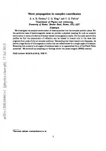
Figure 4: Phase constants - (· · · ) for the discrete model, (—) for the piecewise homogenized model.

0.01

0.005

0 15

16

17

18 19 Frequency (kHz)

20

21

22

Figure 5: Attenuation constants - (−−) for the fully homogenized model, (—) for the piecewise homogenized model.

of the beam segment, which is required to implement the analogous coupling. Once the mechanical and electrical properties are defined, the propagation constants of the transfer matrices in Eqs.(6), (12), (14) and (23) can be compared. For each model, the 8×8 transfer matrices give eight propagation constants µ. Two opposite sets of four constants refer to propagation in opposite directions of the electromechanical waveguide. So, only four propagations constants need to be considered to analyze the phase or the attenuation. First, the phase constants in Fig. 4 show that, below 9 kHz, the discrete model differs significantly from the other ones. Note that the finite element model tends to the piecewise homogenized model when increasing the number of elements. Furthermore, the results obtained with the fully homogenized model are very close to those of the piecewise homogenized model over the frequency range of interest. This is the reason why the fully homogenized and finite element models are not represented in Fig. 4. For each of the other models, only two phase constants are represented because the two other ones are equal to zero. For the piecewise homogenized model, one phase constant approaches a classical beam dispersion relation while the other phase constant reach a step when η = π. This last phase constant thus represents a propagation in a discrete medium [14], which is actually the discrete electrical network. On the other hand, the discrete model offers two phase constants related to discrete waveguides, i.e. with a step at η = π. This is simply explained by the fact that, in the discrete model, the mechanical medium is also represented by a lumped model. Around 7.5 kHz, η = π means that the wavelength is equal to two unit cells and Fig. 4 shows large differences between the models. So, the discrete model is no more valid when the considered wavelength approaches the length of the unit cell. The difference between the piecewise homogenized model and the fully homogenized model clearly appears when looking at the smallest attenuation constant for each model around 19 kHz, as seen in Fig. 5. Over this frequency range, the discrete electrical network does not influence

B. Lossouarn, M. Aucejo, J.-F. De¨u

the results anymore because no ellectrical propagation occurs above 7.5 kHz, which was predicted from Fig. 4. However the effect of the mechanical discontinuity induced by the addition of piezoelectric patches creates a stop band for transverse propagation in the beam. Note that a stop band also appears with the fully homogenized model. This is explained by the fact that, even without considering structural discontinuity, the patches induces additional moments on both sides of the unit cell, as represented in Fig. 2(b). This generates a periodic discontinuity that leads to a moderate stop band effect. This stop band is not negligible compared to the one obtained with the piecewise homogenized model because the effect of the mechanical discontinuity is actually quite small in the present example. With the same geometry, the stop band for longitudinal waves was significant [11], but a similar effect for transverse wave would require a considerably thicker discontinuity. In conclusion, strong structural modification would be needed to benefit from structural stop bands in transverse propagation and, anyway, this effect does not occur on the same frequency range as the proposed analogous control. 4.2

Frequency response functions

Frequency response functions (FRFs) are compared for a free-free beam, which is periodically covered with 20 pairs of piezoelectric patches. The two electrical lines of the network needs to be short-circuited at both ends in order to satisfy analogous boundary conditions [4]. Then, the modal coupling condition tunes the electrical modes to the modes of the discrete mechanical model. A tuned mass control is then observed on several modes together and the vibration amplitude is reduced by introducing damping in the network. Here, a resistance Rs = 20 Ω is added in series to the inductors by replacing L by L − jRs /ω, where j 2 = −1. The finite electromechanical structure consists of n = 20 identical unit cells. A solution to get the relation between the state vectors at both ends of the beam is to raise the transfer matrix to the power of n [4]. The only excitation is a transverse force at one end of the beam. All the other forces, moments and voltages at the ends of the structure are equal to zero. This simplify the problem and it becomes possible to get FRFs as the ratio of the velocity at one end over the excitation force at the other end. The models are first compared in a low-frequency range. The FRFs obtained with the discrete and the piecewise homogenized model are represented in Fig 6 from 0 to 3.3 kHz. This frequency range covers the first eight bending modes of the beam when no coupling occurs. Again, the FRFs obtained with the homogenized and the finite element model are not represented because they cannot be distinguished from the piecewise homogenized model. As predicted by Fig 4, it is observed that the discrete model is no more reliable when the wavelength approaches the length of the unit cell. A limit of validity can be set to 1 kHz, which corresponds to about ten Velocity FRF (dB)

0 −20 −40 −60 −80 0.5

1

1.5 Frequency (kHz)

2

2.5

3

Figure 6: Frequency response functions at low frequencies - (· · · ) for the discrete model, (—) for the piecewise homogenized model.

B. Lossouarn, M. Aucejo, J.-F. De¨u

Velocity FRF (dB)

0 −20 −40 −60 −80 15

16

17

18 19 Frequency (kHz)

20

21

22

Figure 7: Frequency response functions at higher frequencies - (−−) for the fully homogenized model, (—) for the piecewise homogenized model.

unit cells per wavelength according to Fig 4. With the discrete model, the position of the mechanical resonances are shifted because the mechanical medium is modeled by a lattice. Thus, it does not take into account the increasing mistuning between the continuous and the discrete media. The second comparison is performed at higher frequencies. Actually, we want to observe the FRFs when the wavelength in the beam is close to two times the length of a unit cell (η = π). This condition occurs between 18 and 19 kHz and it comes with the stop band effect, which was shown in the analysis of the attenuation constants in Fig 5. The finite element model still tends to the piecewise homogenized model, but the homogenized model now presents a slightly different response, as seen in Fig 7. Below 18 kHz, there is already a difference in the positioning of the resonances, but it is even more pronounced after the stop band, which is larger with the piecewise homogenized model. Nevertheless, the effect of the stop band is quite negligible, especially when considering that the approximations of the Euler-Bernoulli model are questionable at such high frequencies. It is also remarked that the considered frequency range is clearly beyond the last electrical resonances. Here, the control strategy involving an analogous discrete network has no effect and the FRFs are essentially due to propagation in the mechanical waveguide. 5

CONCLUSIONS • Four transfer matrix models are proposed and compared. They differ in the definition of the mechanical medium which can be discrete, fully homogenized, piecewise homogenized or based on a finite element model. • The finite element model tends to the piecewise homogenized model which is the most accurate because it takes into account the mechanical discontinuity induced by the piezoelectric patches. • For problems involving analogous control with a discrete electrical network, the fully homogenized model is generally sufficient because the eventual stop band effects occur at frequencies where the proposed control is no more efficient. • The discrete model is convenient because of its easy implementation but it should be limited to wavelength above ten times the length of the unit cell. • A future work will consist in the extension of the proposed finite element model to the case of a plate coupled to an analogous electrical network.

B. Lossouarn, M. Aucejo, J.-F. De¨u

REFERENCES [1] A. Bloch, Electromechanical analogies and their use for the analysis of mechanical and electromechanical systems. Journal of the Institution of Electrical Engineers-Part I: General, 92, 157–169, 1945. [2] R.H. MacNeal, The solution of partial differential equations by means of electrical networks. California Institute of Technology, 1949. [3] M. Porfiri, F. Dell’Isola, F.M. Frattale Mascioli, Circuit analog of a beam and its application to multimodal vibration damping, using piezoelectric transducers. International Journal of Circuit Theory and Applications, 32, 167–198, 2004. [4] B. Lossouarn, J.-F. De¨u, M. Aucejo, Multimodal vibration damping of a beam with a periodic array of piezoelectric patches connected to a passive electrical network. Smart Materials and Structures, 24, 115037, 2015. [5] D.M. Mead, Wave propagation in continuous periodic structures: research contribution from Southampton. Journal of Sound and Vibration, 190, 495–524, 1996. [6] B.R. Mace, D. Duhamel, M.J. Brennan, L. Hinke, Finite element prediction of wave motion in structural waveguides. The Journal of the Acoustical Society of America, 117, 2835–2843, 2005. [7] L. Airoldi, M. Ruzzene, Design of tunable acoustic metamaterials through periodic arrays of resonant shunted piezos. New Journal of Physics, 13, 113010, 2011. [8] L. Airoldi, M. Ruzzene, Wave Propagation Control in Beams Through Periodic MultiBranch Shunts. Journal of Intelligent Material Systems and Structures, 22, 1567–1579, 2011. [9] G. Wang, S. Chen, J. Wen, Low-frequency locally resonant band gaps induced by arrays of resonant shunts with Antoniou’s circuit: experimental investigation on beams. Smart Materials and Structures, 20, 015026, 2011. [10] Y. Lu, J. Tang, Electromechanical tailoring of structure with periodic piezoelectric circuitry. Journal of Sound and Vibration, 331, 3371–3385, 2012. [11] J.-F. De¨u, B. Lossouarn, M. Aucejo, Comparison of electromechanical transfer matrix models for passive damping involving an array of shunted piezoelectric patches. 22nd International Congress on Sound and Vibration 2015 (ICSV 22), Florence, Italy, June 1216, 2015. [12] C. Maurini, J. Pouget, F. Dell’Isola, Extension of the Euler-Bernoulli model of piezoelectric laminates to include 3D effects via a mixed approach. Computers and Structures, 84, 1438–1458, 2006. [13] O. Thomas, J.-F. De¨u, J. Ducarne, Vibrations of an elastic structure with shunted piezoelectric patches: efficient finite element formulation and electromechanical coupling coefficients. International Journal for Numerical Methods in Engineering, 80, 235–268, 2009. [14] L. Brillouin, Wave propagation in periodic structures. McGraw-Hill, 1946.