TRB-SELEV paper outline - CiteSeerX

Barth/Collins/Scora/Davis/Norbeck

Measuring and Modeling Emissions from Extremely Low Emitting Vehicles Matthew Barth, John Collins, George Scora, Nicole Davis, and Joseph Norbeck Bourns College of Engineering Center for Environmental Research and Technology University of California Riverside, CA 92521 tel: (951) 781-5791, fax: (951) 781-5790

original submission: August 1, 2005 revised November 15, 2005 TRR revision: March 30, 2006 Word count, excluding abstract, references: 5022; figures and tables: 10 * 250 = 2500; total: 7522 Abstract word count: 230

1


2

ABSTRACT In recent years, automobile manufacturers have been producing gasoline-powered vehicles that have very low tailpipe and evaporative emissions in order to meet very stringent certification standards set by the U.S. Environmental Protection Agency and the California Air Resources Board. These extremely low emitting vehicles are 98% to 99% cleaner than catalyst-equipped vehicles produced in the mid 1980s. To better understand the emission characteristics of these extremely low emitting vehicles as well as their potential impact on future air quality, researchers at the University of California, Riverside have conducted a comprehensive study consisting of: 1) an emission measurement program; 2) the development of specific emission models; and 3) the application of future emission inventories to air quality models. Results have shown that in nearly all cases, these vehicles have emissions that are well below their stringent certification standards and continue to have low emissions as they age. Based on the measurement results, new modal emission models have been created for both ULEV- and PZEVcertified vehicles. The model results compare very well to actual measurements. With these models, it is possible to accurately predict future mobile source emission inventories that will have an increasing number of these extremely low emitting vehicles in the overall vehicle population. It is expected that a large penetration of these vehicles in the vehicle fleet will have a significant role in meeting ozone attainment in many regions.


1.

3

INTRODUCTION

Over the last four decades, significant efforts have been made to reduce pollutant emissions from mobile vehicles. Regulatory agencies such as the U.S. Environmental Protection Agency (U.S. EPA) and the California Air Resources Board (CARB) have implemented numerous strategies to reduce mobile source emissions. One of the more successful strategies has been the practice of setting tighter tailpipe and evaporative-emissions certification standards that have been applied over the years to newly manufactured vehicles. For a given model year, a single set of emissions standards applies to all vehicles in specific vehicle classes. Different vehicle classes exist based on engine technology (e.g., gasoline- or diesel-fueled), vehicle weight, and use (e.g., car vs. truck). These emissions have been regulated on a grams-per-mile (g/mi) basis where vehicles are certified on a chassis dynamometer test. The vehicle emission standards have been different between California and the other 49 states, where California has more stringent standards with respect to NOx (oxides of nitrogen) and less stringent standards with respect to CO (carbon monoxide). In recent years, California has aggressively developed and phased-in newer standards as part of their LEV-I and LEV-II programs (1) that are identified as Transitional Low Emission Vehicles (TLEV), Low Emission Vehicles (LEV), Ultra Low Emission Vehicles (ULEV), Super Ultra Low Emission Vehicles (SULEV), and Partial Zero Emission Vehicles (PZEV). The U.S. EPA has also concluded that these more stringent vehicle standards are necessary to meet the National Ambient Air Quality Standards (NAAQS) for ozone and are now phasing similar requirements into their Tier 2 emission standards (2). Over the last several years, vehicle manufacturers have started to introduce vehicles that meet these very tight standards. Although these extremely low emitting vehicles have passed initial certification tests that are performed on laboratory dynamometers, it is unclear whether these vehicles have the same “in-use” emission levels and are durable over time. To better understand the emission characteristics of these extremely low emitting vehicles as well as their potential impact on future air quality, the College of Engineering Center for Environmental Research and Technology (CE-CERT) at the University of California, Riverside has for the past four years conducted a comprehensive study of this new generation of super clean gasoline fueled vehicles. These new vehicles are 98% to 99% cleaner than catalystequipped vehicles produced in the mid 1980s. For purposes of this study, this class of vehicles was designated as “Extremely Low Emitting Vehicles” or “ELEVs,” and the associated study was consequently designated as the “Study of Extremely Low Emitting Vehicles” or the “SELEV” study. This paper highlights several results of this study, with a focus on ULEVs, SULEVs, and PZEVs. To fully understand the real-world environmental impacts of ELEVs, it was important to measure the tailpipe emissions they produce during actual highway, arterial, and residential road driving. This required the development of new portable technologies to measure pollutant emissions from moving vehicles at near zero levels. Unique emissions measurement technology was developed as part of this program and used to test nearly 25 vehicles in different ELEV


4

categories, with different accumulated mileage. Emissions were measured during vehicle startup and while the vehicles were operated in real-world conditions on pre-selected roadways. Another component of the study was to develop emission estimation processes using the acquired data from these vehicles. Sophisticated modal emission models (i.e., models that can predict second-by-second emissions) were developed and subsequently used to calculate large regional emission scenarios for the South Coast Air Basin1 in Southern California. The emission models were used to predict future year emission inventories which were subsequently used as input to air quality models to predict overall air quality impacts. In this paper, several components of the overall SELEV study are described, beginning with the on-road vehicle emission measurement effort. This is followed by a general description of the mobile source emission results and subsequent emissions modeling for these ELEVs. The modeling results are compared to independent measurements as well as other emission models. 2.

EMISSION MEASUREMENT PROGRAM

To characterize the tailpipe emissions from the new generation of ELEVs, vehicles were randomly recruited and thoroughly tested both in the laboratory as well as on-road using a variety of test protocols. In total, 24 vehicles have been recruited and tested, consisting of the certification categories of “Low Emitting Vehicle (LEV)”, “Ultra Low Emitting Vehicle (ULEV)” and “Super Low Emitting Vehicle (SULEV)”, and “Partial Zero Emitting Vehicle (PZEV)”. Note that PZEV vehicles have the same tailpipe certification standards as SULEV vehicles, they only differ in the evaporative emission standards. These vehicles are listed in Table 1. The fuel used during the testing was standard in-use fuel obtained in Southern California and is expected to contain ethanol oxygenate (rather than MTBE oxygenate). Testing occurred in 2002 and 2003 so the fuel used did not meet the California Phase 3 gasoline caps on sulfur. 2.1.

Emission Measurement System

Because the emission levels of these vehicles are so low, standard off-the-shelf measurement equipment could not be used. Instead, specialized on-board emissions measurement instrumentation was developed that could measure at the very low ranges of these vehicles. The on-board instrumentation is centered around a Fourier Transform Infra-Red (FTIR) spectrometer that had custom-built sample extraction and conditioning systems. As part of the overall system, data are also gathered from the vehicle’s On-Board Diagnostics (OBD II) port, a Global Positioning System (GPS) receiver, and ambient condition data acquisition system. Power for all sampling and data acquisition equipment is provided by a battery pack and inverter system that

1 The geographical region encompassing the Los Angeles metropolitan area consists of 186 cities. The east most major cities are Riverside and San Bernardino. Western cities include Long Beach, Santa Monica, Huntington Beach, and Torrance. The South Coast Air Basin is bordered on the north, south, and east by the San Gabriel and San Bernardino mountains and on the west by the Pacific Ocean.


5

allows for approximately 2 hours of operation and imposes no load on the vehicle battery and charging system. Undiluted raw exhaust is withdrawn from the tailpipe through a heated line maintained at 75oC. The sample passes through a quartz filter also heated to 75oC, into a Nafion permeation drier, through the sample pump, and into a second Nafion permeation drier. The first drier is warm due to the heated sample, and rapidly removes the bulk of the water from the sample stream. The second drier is thermoelectrically cooled, which allows it to achieve a low final water content having a dewpoint of about –30oC. The dried sample is then passed to an FTIR gas cell, where pressure is maintained at 900 torr and temperature is maintained at 50oC. The sample leaving the gas cell is combined with nitrogen from a small gas bottle carried on board and used as the purge flow for the Nafion driers. The purge gas is then vented to the atmosphere. The FTIR and sample gas cell consists of an interferometer that is operated with a wavenumber resolution of 0.5 cm-1 through a wavenumber range of 450 to 4000 cm-1, and collects one scan per 1.4 seconds. The gas cell is a white cell design with a path length of 8.28 meters, which for pollutants of interest gives sub-ppm sensitivity. The raw FTIR data are stored during an on-road test, and is post processed using software to generate absorbance spectra which are then quantified. At the sample flow rate provided by the sample conditioning system, the gas cell has a residence time of 15 seconds. This results in a smoothed out concentration signal, too slow to characterize exhaust concentration transients. However, the gas cell is basically a well-mixed flow reactor, which results in an exponential impulse response function. The 15-second exponential time constant can be mathematically compensated for using a digital filter algorithm. Vehicle speed, engine operating characteristics, and geographic position are obtained and logged by the data acquisition system. The engine operating data are used to estimate vehicle exhaust flow rate. Exhaust flow rate is combined with exhaust concentration data to estimate pollutant mass emission rates. Further details on the measurement system are provided in (3). 2.2.

Vehicle Testing Procedure

Each vehicle was tested once on a vehicle chassis dynamometer using specific driving cycles. Initially, the standard Federal Test Procedure (FTP, see (4)) was applied that consists of a cold start portion2, a hot-stabilized running portion, and a warm-start portion. This was followed by a more aggressive US06 driving cycle, which is now used to supplement the FTP for certification purposes (5). Finally, an in-house designed driving cycle was applied, called the MEC01. The MEC01 cycle was developed to exercise the vehicle across its full performance envelope, making it straightforward to extract its modal characteristics (6). The MEC01 cycle was originally developed as part of a larger comprehensive modal emissions modeling program (see (7)).

2

Prior to a “cold start” vehicles are soaked indoors using specific temperature limits as specified by the Code of Federal Regulations for the Federal Test Procedure. The soak period for each vehicle was typically 18 hours.


6

Following the laboratory dynamometer tests, each vehicle was tested extensively on the road. A specific driving course was used that included an initial start, followed by driving on residential roadways, arterial roadways, and freeways. The tests occurred over a three-day period and took place during different times of the day. For the on-road testing, the vehicle carried one driver and the measurement system. The resulting vehicle weight exceeded the certification Equivalent Test Weight (ETW) by 200 to 400 pounds. The same route was driven every time, but the traffic varied from congested to free flowing. 3.

DATA ANALYSIS RESULTS

3.1.

General Results

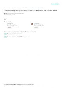
The standard Federal Test Procedure (FTP) test was conducted on a standard dynamometer using the certification equivalent test weight. Emissions were measured using the on-board system. The FTP testing was conducted to verify that the test vehicles were performing according to certification expectations. In the data analysis, two vehicle categories are examined: 1) the ULEV-certified vehicles (which are modeled as a ULEV vehicle/technology category, see Section 4); and 2) the PZEV-certified vehicles, which include both SULEV and PZEV-certified vehicles (since they have the same tailpipe standards). Figure 1a shows the results of FTP testing in weighted grams per mile. Average emission rates are shown for each certification category (ULEV and PZEV) along with error bars showing the variation in the vehicles tested. Also, the ULEV and PZEV standards are shown as black bars in the graphs. It can be seen that for all species of emissions (NMHC (non-methane hydrocarbons), CO (carbon monoxide), and NOx (oxides of nitrogen)), these vehicles are below the certification standards. The figure also shows that the PZEV vehicles have significantly lower emissions compared to the ULEV vehicles, as expected. Figure 1b shows the emissions measured during testing over the US06 drive cycle. The US06 cycle contains aggressive freeway driving and is one component of the Supplemental Federal Test Procedure (SFTP, see (4)). At the time of the testing, not all of the vehicles were certified to meet the SFTP standard which was being phased over the model years 2001 through 2004. As a result, this figure shows great variability (i.e., large error bars) for each average emissions species. For the most part, the emissions were below the US06 standards. In order to better understand the effects of low vs. high mileage, the ULEV vehicles were subsequently separated into two groups, one that had low mileage (i.e., < 50K miles) and another that had higher mileage (i.e., > 50K miles). The certification standards are relaxed for the higher mileage vehicles, as shown in Figure 2. In this figure the lower mileage vehicles had lower emissions than the higher mileage vehicles. In all cases, the tested vehicles were below the certification standards. 3.2.

On-Road Hot Running and Cold-Start Effects

For the on-road testing, it was seen that the emission rates are higher during the cold start as expected, then fall off to low values once the catalyst lights off. The low values are a


7

combination of near-zero emission rates with frequent small emission spikes and infrequent moderate to large emission spikes. The emission spikes occur in response to driving events, but they occur randomly enough that it makes sense to speak of average hot running emission rates. Figure 3a shows the average hot running emission rates for the two categories of vehicles. The error-bars show the vehicle-to-vehicle as well as test-to-test variability expressed as one standard deviation. The hot running emission rates were calculated starting from 300 seconds after ignition and continuing through the end of the test. Thus, the hot running emission rates are averages over the combined freeway, arterial, and residential sections. Note that actual running emission rates for these vehicles are well below the certification emission rates. Examining the second-by-second nature of the emissions, it was generally seen that the emissions levels stay very low under very moderate driving conditions, and occasionally spike during short highdemand power periods. Start emissions were also examined in detail, focusing on the first 300 seconds of the on-road driving tests. The results, shown in Figure 3b, show substantial test-to-test variability, particularly in NOx. This is primarily due to the sensitivity to slight differences in power demand during the early portions of the test when the vehicle is not warmed up yet. Part of the variability is also due to variation in traffic and power demand. The cutoff of 300 seconds was chosen to ensure that the catalyst was fully operational and that the emissions that follow are hot-running. Many of the vehicles reached their hot stabilized condition within 60 to 100 seconds. For the PZEV-certified vehicles, nearly all the NMHC emissions occur during the start. For the ULEV vehicles, the majority of the NMHC emissions occur during the start, but there are also periods of time near the beginning and end of the tests showing significant NMHC emissions. In regards to NOx emissions, it was noted that ULEV vehicles had NOx significantly higher than PZEV vehicles. Similar to NMHC, the start emissions for some vehicles vary substantially with soak time, with shorter soak times having higher emissions. After the start, the cumulative NOx emissions tend to look like stair steps, which mean that relatively long periods of low NOx emissions are being frequently interspersed with short spikes of high NOx emissions. Even though the running emissions are occurring in brief spikes, they occur frequently enough to impart an overall trend or slope to a cumulative emission plot. Periods of steep slope have larger and more frequent emission spikes. These are periods associated with freeway and aggressive driving. Based on the testing, it was seen that PZEV vehicles sometimes produce large CO spikes. These spikes occur during transients under very high power demand. For example, during a hard uphill acceleration, the driver momentarily reduces the pressure on the accelerator pedal then immediately resumes acceleration. This type of event can affect the response of the engine control management, which was anticipating continued reduction of power demand. CO concentrations during these events can reach several percent CO by volume. These events appear to be more common in PZEVs than in ULEVs, and more common in ULEVs than in LEVs. In general, the more finely tuned the emission control system, the more it is susceptible to power spikes. It is important to point out however, that even with the CO emission spikes, the emissions are generally well below the certification levels.


4.

MODELING

4.1.

Modal Modeling

8

As part of the SELEV program, modal emissions models have been developed for both ULEV and SELEV vehicles, as part of UC Riverside’s Comprehensive Modal Emissions Modeling (CMEM) framework (6). CMEM was originally developed at the University of CaliforniaRiverside along with researchers from the University of Michigan and Lawrence Berkeley National Laboratory through an NCHRP (National Cooperative Highway Research Program) research project that originally started in August of 1995. The overall objective of CMEM is to develop and verify a modal emissions model that accurately reflects mobile-source emissions produced as a function of the vehicle’s operating mode. The model is comprehensive in the sense that it is able to predict emissions for a wide variety of vehicles in various states of condition (e.g., properly functioning, deteriorated, malfunctioning). The model is capable of predicting second-by-second tailpipe (and engine-out) emissions and fuel consumption for a wide range of vehicle/technology categories. Originally, CMEM was targeted at light-duty vehicles (LDVs, i.e., cars and small trucks) but has since been expanded to many other vehicle/technology categories. CMEM uses a physical, power-demand modal modeling approach based on a parameterized analytical representation of emissions production. In such a physical model, the entire emissions process is broken down into different components that correspond to physical phenomena associated with vehicle operation and emissions production. Each component is then modeled as an analytical representation consisting of various parameters that are characteristic of the process. These parameters typically vary according to the vehicle type, engine, and emissions technology. Many of these parameters are stated as specifications by the vehicle manufacturers, and are readily available (e.g., vehicle mass, engine size, and transmission type). Other key parameters relating to vehicle operation and emissions production must be deduced from actual second-by-second measured emissions data. The basic components found in the model instances include a power demand component, engine speed estimator, fuel rate model, engine-out emission component, and an after-treatment component (8). Also part of the model are specific components that mimic engine strategies that control fuel/air equivalency ratios or fuel injection timing. This type of modeling is considered more deterministic rather than descriptive. Such a deterministic model is based on causal parameters or variables, rather than based on simply observing the effects (i.e., emissions) and assigning them to statistical bins (i.e., a descriptive model). This approach provides understanding, or explanation, for the variations in emissions among vehicles, types of driving, and other conditions. Using this type of model, analysts can gain insight to the physical and chemical reasons behind this model of emissions production. The physical modal emissions modeling approach has several attractive attributes including 1) It inherently handles all of the factors in the vehicle-operating environment that affect emissions, such as vehicle technology, fuel type, operating modes, maintenance, accessory use, and road grade; 2) It is applicable to all vehicle and technology types such that when modeling a heterogeneous vehicle population, separate sets of parameters can be used within the model to


9

represent all vehicle and technology types. The total emissions outputs of the different classes can then be integrated with their correctly weighted proportions to create an entire emissions inventory; and 3) It is not restricted to pure steady-state emissions events, as is an emissions map approach. Emissions events that are related to the transient operation of the vehicle can be appropriately modeled. Further, it can easily handle time dependence in the emissions response to the vehicle operation. As stated previously, the operating history (i.e., the last few seconds of vehicle operation) can play a significant role in an instantaneous emissions value. More detailed discussions about modal emissions modeling and CMEM can be found in (6), (7), (8), (9). 4.2.

Architecture and Parameter Adjustments

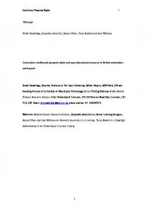
In the developed modal emissions model, second-by-second vehicle tailpipe emissions are modeled as the product of three components: fuel rate (FR), engine-out emission indices (gemission/gfuel), and time-dependent catalyst pass fraction (CPF): Tailpipe Emissions = FR ● (gemission/gfuel) ● CPF Here FR is fuel use rate in grams/s, engine-out emission index is grams of engine-out emissions per gram of fuel consumed, and CPF is the catalyst pass fraction, which is defined as the ratio of tailpipe to engine-out emissions. CPF usually is a function primarily of fuel/air ratio and engineout emissions. As shown in Figure 4, the generalized model consists of six distinct modules that individually predict: 1) engine power; 2) engine speed; 3) air/fuel ratio; 4) fuel use; 5) engine-out emissions; and 6) catalyst pass fraction. Details of the model structure are given in [An et al, 1997]. For each sub-model, there are a number of vehicle parameters and operating variables that are considered. The vehicle parameters used are divided into two groups: 1) parameters that are obtained from the public domain (or determined generically), and 2) parameters that need to be calibrated based on the second-by-second emission measurements. Examples of the first group include vehicle mass, engine displacement, rated engine power and torque, etc. Examples of the second group include engine friction factor, enrichment threshold and strength, catalyst pass fraction, etc. Emission modeling of different vehicle/technology categories within this architecture requires category specific calibration of the second group of model parameters mentioned above. For each vehicle/technology category, a different model “instance” or sub-model has been created using a parameterized physical approach (see (7)). Based on the results of this SELEV program, two new vehicle/technology categories have been added to CMEM. One of the categories corresponds to ULEV-certified vehicles, the other corresponds to SULEV and PZEV-certified vehicles. For these two vehicle/technology categories, major architectural changes were not required and modeling of these new extremely low emitting vehicle categories resulted in new sets of calibration parameters. There are several factors that contribute to low ELEV emissions. One of the most important is catalyst performance. The most relevant catalyst characteristics, from a modeling perspective,


10

are catalyst light-off-times and hot running catalyst efficiencies. Test data show that for extremely low emitting vehicles most of the emissions are generated during the startup period (cold- and warm-starts). For this reason, the light-off-time parameter has one of the largest impacts on total emissions. Based on measured light-off data illustrated in Figure 5, ELEV emission control systems will have increasingly shorter light off times. This is one of the biggest parameter changes in the CMEM LDV modeling. In addition to shorter light-off-times, ELEV vehicles exhibit very high stabilized catalyst efficiency during hot running operation. For the ELEV CMEM modeling, catalyst efficiency parameters are significantly different when compared to Tier 0 and Tier 1 vehicles. ELEV emission values are also a result of improvements in the control of engine operating conditions, most notably in fuel enrichment and enleanment. Enleanment is generally associated with increases in NOx and in some cases HC emissions. Enrichment results in increased CO emissions. CMEM estimates open loop or fuel-enrichment operation based on a power threshold level, which has been steadily increasing with newer vehicles. In CMEM, this power threshold level is a calibrated parameter and is significant higher for ELEVs when compared to other vehicle/technology categories. CMEM estimates when significant enleanment occurs based on a calibrated enleanment parameter and engine-out emissions. Differences have been noted in the enleanment parameters between ELEVs and other vehicle types. With the exception of hydrocarbon absorbers, the major improvements in ELEV emission control technology can be represented well with the existing CMEM architecture. CMEM has sophisticated cold-start and catalyst efficiency sub-models with several parameters that can be calibrated to give quicker catalyst light off times and stabilized hot running catalyst efficiencies. Catalyst efficiency is based on a calibrated maximum catalyst efficiency which is near 100 for ELEV vehicles, cumulative fuel use used as a surrogate for catalyst temperature, and a calibrated cold start catalyst coefficient specific to each pollutant. Additionally, catalyst warm start is also modeled based on cumulative fuel use and several calibrated cold start catalyst parameters. Calibration of vehicle category parameters is automated using an optimization routine that minimizes measured and modeled differences for variations in selected parameters across selected data sets. Hydrocarbon absorption is another means of obtaining extremely low tailpipe emissions and was clearly identified in at least one of the test vehicles. However, not all ELEV vehicles had this characteristic and therefore it was not specifically modeled. A future modeling task may be to create a sub-category of ELEV vehicles that specifically utilize hydrocarbon absorption. This phenomenon can be modeled in much the same way that unburned hydrocarbon emissions are modeled in the existing CMEM architecture (8). 4.3.

Model Validation

Model validation is an essential step in the modeling process. As an example of how the modeled predictions match the measurements, Figure 6 shows second-by-second emissions for modeled (red) and measured (blue) for tailpipe CO2, CO, HC and NOx emissions for a single vehicle


11

(ULEV08). The numbers to the right of the plot from top to bottom are total measured emissions over the cycle, total modeled emissions over the cycle, and the percent difference between the two. This particular vehicle above was generally well behaved although there are a few NOx emission events that the model was unable to capture. The validation of CMEM’s SELEV categories presented in this paper is not completely independent of the calibration data. Calibration was done based on portions of the MEC and FTP cycles selected to represent specific modes of operation. One set of parameters for each vehicle category was optimized to best predict emissions for the various driving cycle portions. Results for both cycles in their entirety were then calculated and combined as a measure of validity. From a larger perspective, Figure 7 shows composite comparison results for all the vehicles by technology category. These data include both the dynamometer test (FTP and MEC01 drive cycles) as well as a portion of the on-road data. This figure shows that there are some discrepancies between modeled and measured ELEV emissions, particularly for NOx and CO. However, these differences are no greater than +/- 5% for ULEVs and +/- 15% for SULEVs. A likely cause for the SULEV discrepancy is the fact that these vehicle’s cumulative emissions across the cycles are so small that even small fluctuations in emissions predictions can result in large errors. 4.4.

Conventional Model Comparison

In addition to creating a modal emissions model, overall emission rates from the testing program were compared to current existing emission models such as CARB’s EMFAC model, see (10). Emissions data (both dynamometer and on-road) from the ULEV vehicles described in Section 2 were compared with existing emission factors and the standards. The emissions for all tested vehicles were below the certification standard with the exception for NOx, see Figure 8. Both measured NMHC and CO were lower than the FTP composite emissions used in the EMFAC model. Measured NOx was higher than assumed in EMFAC for the FTP composite cycle. It is important to note that the EMFAC model emission rates were developed before ELEV vehicles were available for testing, therefore the rates were assumed to be proportional to the standards. Considering the simplicity of this technique, it appears that EMFAC does a reasonable job at estimating FTP emissions from the ULEV vehicles. The emissions models should not only to predict FTP cycle emissions, but more importantly are needed to provide an accurate estimate of real world emissions, which can be very different than emissions from the FTP cycle. Figure 9a shows the performance of the ULEVs during the FTP cycle and during actual on-road driving conditions, along with current model predictions. The term BER (Base Emission Rate) refers to the primary emissions input into the EMFAC model. For running emissions, the BER is equivalent to Bag 2 of the FTP. For starts, the BER can roughly be compared to Bag 1-Bag3 of the FTP. The CARB defines start emissions as the emissions occurring in the first 100 seconds of operation. To be consistent with the CARB’s methodology, on-road measured start emissions are defined to be emissions occurring in the first 100 seconds of vehicle operation, as opposed to the 300 seconds used in Section 2. The difference between the BER modeled and the on-road modeled are that driving correction factors


12

and other modifications are applied to the BER in the EMFAC model to estimate on-road emissions. All modeled values were obtained from the CARB’s EMFAC2002 version 2.2 (10). On-road measured and on-road modeled emissions in Figure 9a represent typical running emissions from a combination of arterial and freeway driving. The speed distribution observed in the measured on-road driving course was input to the on-road modeled emissions in EMFAC. Likewise, the ambient temperature, humidity, and other environmental effects were used in EMFAC to most closely represent the measured conditions for the on-road testing of the ULEVs. Average running emissions were much lower than predicted for CO and HC, as shown in Figure 9a. Average start emissions were in general higher than predicted for both the BER and from onroad start emissions, as shown in Figure 9b. 5.

CONCLUSIONS AND FUTURE WORK

In order to better understand today’s extremely low emitting vehicles, UCR CE-CERT has carried out a comprehensive measurement and modeling study focused on these vehicles. Nearly 25 vehicles were extensively tested and subsequently modeled. Several key conclusions can be drawn: •

The study has shown that publicly-owned, in-use ELEVs are meeting performance expectations in Southern California, both at introduction and at high accumulated mileage;

•

High speed driving can lead to dramatic increases in on-road emissions for some of the ELEVs, but most of these vehicles were not designed to meet the SFTP high-speed driving standards. The on-road testing portion of the program has shown that SFTPcertified ELEVs meet performance expectations in Southern California freeway driving.

•

The SFTP experience has showed the potentially large sensitivity of ELEV emissions to test conditions outside the calibration envelope.

•

On-road and laboratory ELEV measurements confirmed that actual on-road driving emissions are different than emissions from the FTP cycle. As a result, the modeling performance of conventional models to model on-road driving is problematic.

•

Current regulatory emissions models (such as EMFAC) do a reasonable job at an order of magnitude emission estimate for overall on-road driving from ELEVs. However, this model does a poor job at predicting component behavior. For example, EMFAC typically significantly overestimates running emissions and underestimates start emissions for the ELEVs. Updating the modeling approach with actual data instead of standard based emission factors will significantly improve model performance.

•

A physical modal emissions model (such as CMEM) can be used to sufficiently model these ELEVs without major architecture changes; major changes occur in parameters such as catalyst light-off time, hot-running catalyst efficiency, and enrichment power


13

thresholds. Modeled emissions compare favorably to measured emissions for overall emissions predictions as well as for predicting individual on-road driving components. Another component of the SELEV program is to quantify the air quality effects of ELEVs at large regional scales. It is desired to determine the (ozone) air quality impact from the introduction and penetration of these ELEVs in to the vehicle population. The results of this study are forthcoming in another publication. ACKNOWLEDGEMENTS The authors would like to acknowledge the people involved in the testing and data handling portion of this project and others who have been associated with the SELEV program. This work has been sponsored in part by Honda Motor Company, the U.S. EPA, the California Air Resources Board, Chevron-Texaco, and the Manufacturers of Emission Controls Association (MECA). The contents of this paper reflect the views of the authors and does not necessarily indicate acceptance by the sponsors. REFERENCES (1)

California Air Resources Board (CARB) “Formal Regulatory Documents for LEV-II Regulations” web site: http://www.arb.ca.gov/msprog/levprog/levii/levii.htm; accessed July 2005.

(2)

U.S. Environmental Protection Agency (U.S. EPA) “National Ambient Air Quality Standards (NAAQS)”, see web site http://www.epa.gov/air/criteria.html, accessed July 2005.

(3)

Truex, T., J. Collins, J. Jetter, B. Knight, T. Hayashi, N. Kishi, and N. Suzuki (2000) “Measurement of Ambient Roadway and Vehicle Exhaust Emissions-An Assessment of Instrument Capability and Initial On-Road Test Results with an Advanced Low Emission Vehicle”, Society of Automotive Engineers, Technical Paper #SAE 2000-01-1142.

(4)

FTP. 1989. Code of Federal Regulations. Title 40. Parts 86-99 (portion of CFR which contains the Federal Test Procedure), Office of the Federal Register.

(5)

U.S. EPA. 1995. Regulatory Impact Analysis, Federal Test Procedure Revisions. Office of Mobile Sources, Office of Air and Radiation, US Environmental Protection Agency.

(6)

Barth, M., T. Younglove, T. Wenzel, G. Scora, F. An, M. Ross, and J. Norbeck. 1997. “Analysis of modal emissions from diverse in-use vehicle fleet”. Transportation Research Record No. 1587, pp 73-84, Transportation Research Board, National Academy of Science.

(7)

Barth, M., F. An, T. Younglove, C. Levine, G. Scora, M. Ross, and T. Wenzel. (1999) “The Development of a Comprehensive Modal Emissions Model”. Final report submitted to the National Cooperative Highway Research Program, November, 1999, 255 p.


14

(8)

An, F., M. Barth, M. Ross and J. Norbeck. (1997) “The Development of a Comprehensive Modal Emissions Model: Operating Under Hot-Stabilized Conditions”. Transportation Research Board Record Series 1587: 52-62, Washington DC, 1997.

(9)

Barth, M., F. An, J. Norbeck and M. Ross. (1996) “Modal Emissions Modeling: A Physical Approach”, Transportation Research Board Record Series 1520: 81-88.

(10) California Air Resources Board (CARB) (2005) “Motor Vehicle Emissions Inventory Modeling Suite”, see web site: http://www.arb.ca.gov/msei/msei.htm; accessed July 2005.


15

LIST OF TABLES AND FIGURES

Table 1. List of Vehicles tested in program. Figure 1. a) FTP weighted emissions during dynamometer testing; b) US06 emissions during dynamometer testing. Figure 2. Weighted FTP emissions for ULEV vehicles, grouped into low- and high-mileage groups. Figure 3. a) On-road hot running (g/mi) emissions test results for ULEV and PZEV categories; b) On-road cold start emissions (grams in 300 seconds). Figure 4. Modal emissions model architecture for light duty vehicles. Figure 5. Average Time to Reach Optimum HC Catalyst Efficiency During FTP Cycle. Figure 6. Second-by-second comparison of measured (blue) and modeled (red) emissions for vehicle ULEV08 operating over the FTP driving cycle. Figure 7. Composite comparison results between measured and modeled ELEVs. Figure 8. Comparison of Measured and Modeled FTP Composite Emissions. Figure 9. a) Measured and Modeled Running Emissions Comparison from ULEV vehicles. b) Measured and Modeled Start Emissions Comparison from ULEV vehicles.

16


Table 1. List of Vehicles tested in program Certification Year LEV 2001 ULEV 1999 ULEV 2000 ULEV 2001 ULEV 2001 ULEV 2001 ULEV 2001 ULEV 2002 ULEV 2002 ULEV 2002 ULEV 2002 ULEV 2002 ULEV 2002 ULEV 2002 ULEV 2002 ULEV 2002 ULEV 2003 ULEV 2003 SULEV 2000 SULEV 2001 PZEV 2003 PZEV 2003 PZEV 2003 PZEV 2003

Make Model Odometer Chevrolet Malibu 11,324 Honda Accord LX 80,124 Dodge Neon 87,608 Ford Focus 35,089 Honda Accord LX 5,500 Mazda Protégé 27,114 Volkswagen Jetta GLS 88,790 Acura 3.2TL 32,344 Buick Regal 21,184 Ford Mustang 23,894 Honda Civic 26,632 Mitsubishi Galant 22,350 Mitsubishi Lancer 13,300 Nissan Altima 13,747 Saturn L200 14,888 Toyota Camry LE 13,098 Honda Civic Hybrid 13,700 Toyota Corolla 21,835 Honda Accord EX-L 7,000 Nissan Sentra CA 3,863 Honda Accord EX 7,731 Honda Civic GX 15,191 Honda Civic Hybrid 1,502 Toyota Camry LE 2,600

17


0.140

ULEV NOx Std. Is offscale

ULEV CO Std. Is offscale

0.120

PZEV Std.

a)

Weighted FTP Emissions (g/mi)

0.100

0.080 ULEV PZEV 0.060

ULEV Std.

0.040

PZEV Std.

0.020

PZEV Std.

0.000 NMHC

CO/10

NOx

0.250

b)

US06 Emissions (g/mi)

0.200

0.150

US06 Std.

ULEV PZEV 0.100 US06 Std.

0.050

0.000 NMHC

CO/100

NOx

NMHC+NOx

Figure 1. a) FTP weighted emissions during dynamometer testing; b) US06 emissions during dynamometer testing

18


Weighted Emissions (g/mi)

0.5

1.7 g/mi

2.1 g/mi

CO standards are offscale

0.4 Low Miles High Miles ULEV Std (new) ULEV Std (50K)

0.3 0.2 0.1 0.0 CO

NOx

NMHC

Figure 2. Weighted FTP emissions for ULEV vehicles, grouped into low- and high-mileage groups.

19


0.120

a)

On-road, Hot-running Emissions (g/mi)

0.100

0.080

0.060 ULEV PZEV

0.040

0.020

0.000 CO/10

NMHC

NOx

-0.020

0.700

b)

On-Road, Cold-Start Emissions (g/start)

0.600

0.500

0.400 ULEV PZEV

0.300

0.200

0.100

0.000 CO/10

NMHC

NOx

-0.100

Figure 3. a) On-road hot running (g/mi) emissions test results for ULEV and PZEV categories; b) On-road cold start emissions (grams in 300 seconds).

20


(2) ENGINE SPEED (N)

(A) INPUT OPERATING VARIABLES (1) POWER DEMAND (B) MODEL PARAMETERS

(4) FUEL RATE (FR) (3) AIR/FUEL EQU. RATIO (Φ)

(5) ENGINEOUT EMISSIONS

TAILPIPE EMISSIONS (6) & CATALYST FUEL USE PASS FRACTION

b. Stoichiometric c. Enrichment d. Enleanment a. Soak time

Figure 4. Modal emissions model architecture for light duty vehicles.

21


Time (seconds)

120 100 80 60 40 20 0 Tier 0

Tier 1

LEV

ULEV

SULEV

Vehicle Type

Figure 5. Average Time to Reach Optimum HC Catalyst Efficiency During FTP Cycle

Figure 6. Second-by-second comparison of measured (blue) and modeled (red) emissions for vehicle ULEV08 operating over the FTP driving cycle.

22

Measured - Modeled % Difference


15.0 10.0 5.0 lev ulev sulev

0.0

NOx

HC

CO2

CO

-5.0 -10.0 -15.0 Figure 7. Composite comparison results between measured and modeled ELEVs.

0.25 Standard

FTP composite emissions (g/mi)

Measured (max)

0.2

Measured (ave) EMFAC

0.15

0.1

0.05

0 NMHC

CO/10

NOx

Figure 8. Comparison of Measured and Modeled FTP Composite Emissions.

23


0.12

BER Measured On-Road Measured

0.10

BER Modeled

Emissions (g/mi)

On-road Modeled

a)

0.08

0.06

0.04

0.02

0.00 NMHC 0.5

CO/10

NOx

BER Measured On-Road Measured BER Modeled

Emissions (g/start

0.4

b)

On-road Modeled

0.3

0.2

0.1

0.0 NMHC

CO/10

NOx

Figure 9. a) Measured and Modeled Running Emissions Comparison from ULEV vehicles. b) Measured and Modeled Start Emissions Comparison from ULEV vehicles