Tree-Based Algorithms for Protein Classification R´obert Busa-Fekete1 , Andr´as Kocsor1,2,3 and S´andor Pongor4,5 1
2
3 4
5
Research Group on Artificial Intelligence of the Hungarian Academy of Sciences and University of Szeged, Aradi v´ertan´ uk tere 1., H-6720 Szeged, Hungary E-mail: {busarobi, kocsor}@inf.u-szeged.hu Research Group on Artificial Intelligence NPC., Pet˝ ofi S. Sgt. 43., H-6725 Szeged, Hungary Applied Intelligence Laboratory Ltd., Pet˝ ofi S. Sgt. 43., H-6725 Szeged, Hungary Bioinformatics Group, International Centre for Genetic Engineering and Biotechnology, Padriciano 99, I-34012 Trieste, Italy E-mail:
[email protected] Bioinformatics Group, Biological Research Centre, Hungarian Academy of Sciences, Temesv´ ari krt. 62, H-6701 Szeged, Hungary
Summary. The problem of protein sequence classification is one of the crucial tasks in the interpretation of genomic data. Many high-throughput systems were developed with the aim of categorizing the proteins based only on their sequences. However, modelling how the proteins have evolved can also help in the classification task of sequenced data. Hence the phylogenetic analysis has gained importance in the field of protein classification. This approach does not just rely on the similarities in sequences, but it also considers the phylogenetic information stored in a tree (e.g. in a phylogenetic tree). Eisen used firstly phylogenetic trees in protein classification, and his work has revived the discipline of phylogenomics. In this chapter we provide an overview about this area, and in addition we propose two algorithms that well suited to this scope. We present two algorithms that are based on a weighted binary tree representation of protein similarity data. TreeInsert assigns the class label to the query by determining a minimum cost necessary to insert the query in the (precomputed) trees representing the various classes. Then TreNN assigns the label to the query based on an analysis of the query’s neighborhood within a binary tree containing members of the known classes. The algorithms were tested in combination with various sequence similarity scoring methods (BLAST, Smith-Waterman, Local Alignment Kernel as well as various compression-based distance scores) using a large number of classification tasks representing various degrees of difficulty. At the expense of a small computational overhead, both TreeNN and TreeInsert exceed the performance of simple similarity search (1NN) as determined by ROC analysis, at the expense of a modest computational overhead. Combined with a fast tree-building method, both algorithms are suitable for web-based server applications.
Key words: Proteomics, Protein classification, Phylogenetics, Phylogenomics
2
Busa-Fekete et. al.
1 Introduction The categorization of biological objects is one of the fundamental and traditional tasks of the life sciences. For instance, the categorization of organisms into a hierarchical ”Tree of life” leads to a complex model that summarizes not just the taxonomic relationships between the species, but also the putative time-course of evolution as we understand it today. With the advent of molecular biology in the 1970’s, the categorization of genes and proteins itself became an important subject of research. Sequences of individual proteins can for instance be compared using string distance measures, and one can build trees that closely resemble the hypothetical ”Tree of life”. The categorization of protein structures, on the other hand, began from a different perspective: protein structures reveal a few fundamental molecular arrangements (like alpha-helices and beta-sheets) that can combine in a variety of ways and give rise to characteristic molecular shapes. Finally, the recent advent of genomics research - the wholesale analysis of the gene and protein repertoire of a species - led to yet another perspective with an emphasis on biological function. According to this approach, the known genes/proteins are categorized into a priori determined, empirical categories that reflect our current knowledge on the cellular and biochemical functions. As proteins carry many, perhaps most of the known biological functions, they play a prominent role in the functional analysis of genomes. The methods of protein classification fall into three broad categories: i) Methods based on pairwise comparison, i.e. ones that work by comparing an unknown object (protein sequence or structure) with members of an a priori classified database of protein objects. The results are ranked according to the similarities and the strongest similarities are evaluated in terms of biological or statistical significance, after which a query is assigned to the class of the most similar object. ii) Methods based on consensus (or aggregate) descriptions, i.e. ones that are used to analyze distant sequence similarities that cannot readily be determined based on a simple similarity analysis. Here we first prepare a consensus description for all the classes of a protein sequence database, then we compare the unknown query with each of the consensus descriptions. As with the previous methods, the strongest similarities are evaluated and used to assign the protein to the given class. There are various methods for preparing consensus descriptions, including regular expressions, frequency matrices and Hidden Markov Models. The above methods are described in textbooks and are periodically reviewed. iii) A more recent type of protein classification methods attempts to use an external source of knowledge in order to increase the classification sensitivity. The external source of knowledge is the phylogenetic classification of an organism, i.e. the knowledge that is accumulated in the fields of taxonomy and molecular phylogeny. This approach is called phylogenomics (for a recent review see [1]) and is closely linked to the notions of orthologs (proteins that share both ancestry and function) and paralogs (proteins that share a common ancestry but carry different functions). The
Tree-Based Algorithms for Protein Classification
3
practical goal of phylogenomics is to reveal the true orthologous relationships and use them in the process of classification. Like ii), phylogenomic methods are used for distant similarities that cannot be decided by simple comparisons like those mentioned in i). The aim of the present chapter is to describe two protein classification algorithms that make use of tree structures. The chief difficulties of protein classification arise from the fact that the databases are large, noisy, heterogeneous and redundant; that the classes themselves are very different in terms of most of their characteristics; that the assignments are often uncertain. For these reasons there is a constant need for better and faster algorithms that can cope with the growing datasets, and tree-based approaches are promising in this respect [2]. Even though trees are often used in molecular phylogenies and phylogenomics, the motivation of our work is quite different since we are not trying to reveal or to use the taxonomic relationships between species or proteins. We employ trees - especially weighted binary trees - as a simple and computationally inexpensive formalism to capture the hidden structure of the data and to use it for protein classification . The rest of this chapter is structured as follows. Section 2 provides a brief overview of related work, with a strong focus on the protein comparison and tree-building methods used here. Afterwards Sections 3 and 4 respectively describe the two algorithms called TreeNN and TreeInsert. TreeNN (Section 3) is based on the concept of a distance that can be defined between leaves of a weighted binary tree. TreeNN is a pairwise comparison type algorithm (see i) above), where the distance function incorporates information encoded in a tree structure. Given a query protein and an a priori classified database, the algorithm first constructs a common tree that includes the members of the database and the query protein. In the subsequent step the algorithm attempts to assign labels to an unknown protein using the known class labels found in its neighborhood within the tree. A weighting scheme is applied, and the class label with the highest weight is assigned to the query. TreeInsert (Section 4) is based on the concept of tree insertion cost, this being a numerical value characterizing the insertion of a new leaf at a given point of a weighted binary tree. The algorithm finds the point with minimum insertion cost in a tree. TreeInsert uses the tree as a consensus representation so it is related to the algorithms described above in ii). Given an unknown protein and protein classes represented by precalculated weighted binary trees, the query is assigned to the tree into which it can be inserted at the smallest cost. In the description of both algorithms we first give a conceptual outline that summarizes the theory as well as its relation to the existing approaches i-iii. This is followed by the formal description of the algorithm, the principle of the implementation, and some possible heuristic improvements. Then we round off the paper with a brief discussion and some conclusions in Section 5. As for the databases and the classification tasks used for benchmarking the algorithms, these are described in the Appendix.
4
Busa-Fekete et. al.
2 Related work The algorithms described in this work belong to the broad area of protein classification , and have been summarized in several recent reviews and monographs [3]. In particular, we will employ the tools developed for protein sequence comparison that are now routinely used by researchers in various biological fields. The Smith-Waterman [4] and the Needleman-Wunsch algorithms [5] are exhaustive sequence comparison algorithms, while BLAST [6] is a fast heuristic algorithm. All of these programs calculate a similarity score that is high for similar or identical sequences and zero or below some threshold for very different sequences. Methods of molecular phylogeny build trees from the similarity scores obtained from the pairwise comparison of a set of protein sequences. The current methods of tree building are summarized in the splendid textbook by J. Felsenstein[7]. One class of tree/building methods the so-called distance based methods are particularly relevant to our work since we use one of the simplest method, namely Neighbour-Joining (NJ) [8], to generate trees from the data. Protein classification supported by phylogenetic information is sometimes termed phylogenomics [1, 9]. The term covers an eclectic set of tools that combine phylogenetic trees and external data-sources in order to increase the sensitivity of protein classification [1]. Jonathan Eisen’s review provides a conceptual framework for combining functional and phylogenetic information and describes a number of cases where functions cannot be predicted using sequence similarity alone. Most of the work summarized by Eisen is devoted to the human evaluation of small datasets by hand. The first automated annotation algorithm was introduced by Zmasek and Eddy [10] who used explicit phylogenetic inference in conjunction with real-life databases. Their method applies the gene tree and the species tree in a parallel fashion, and it can infer speciation and duplication events by comparing ¡ ¢the two distinct trees. The worst case running time of this methods is O n2 , and the authors used the COG dataset [11] to show that their method is applicable for automated gene annotation. Not long ago Lazareva-Ulitsky et. al. employed an explicit measure to describe the compatibility of a phylogenetic tree and a functional classification [12]. Given a phylogenetic tree overlaid with labels of functional classes, the authors analyzed the subtrees that contain all members of a given class. A subtree is called perfect if its leaves all belong to the one functional class and an ideal phylogenetic tree is made up of just perfect subtrees. In the absence of such a perfect subdivision, one can establish an optimal division i.e. one can find subtrees that contain the least ”false” labels. The authors defined a so-called tree measure that characterizes the fit between the phylogenetic tree and the functional classification, and then used it to develop a tree-building algorithm based on agglomerative clustering. For a comprehensive review on protein classification see [1].
Tree-Based Algorithms for Protein Classification
5
3 TreeNN : Protein classification via neighborhood evaluation within weighted binary trees 3.1 Conceptual outline Given a database of a priori classified proteins that are compared to each other in terms of a similarity/dissimilarity measure6 , and a query protein that is compared to the same database in terms of the same similarity/dissimilarity measure, one can build a weighted, binary tree that will contain proteins in each leaf. If we now assign the known class labels to the proteins, all leaves except the unknown query will be labelled, as schematically shown in Figure 1.
Fig. 1. A weighted tree of proteins overlayed with class labels.
First let us denote the length of the unique path between two leaves Li and Lj by p (Li , Lj ). Here p (Li , Lj ) is an integer representing the number of edges along the path between Li and Lj . We can define the closest neighbourhood K (L) of a leaf L as the set of leaves for which there is no Lj leaf such that p (L, Lj ) < p (L, Li ). For instance the closest neighbours of q in Figure 1 are both members of class 2 and are three steps apart from q. These leaves are parts of the 3-neighbourhood of q (i.e. the set of leaves for which the path between q and them at the most 3). If the tree is a weighted binary tree we can define the leaf distance l (Li , Lj ) between two leaves Li and Lj as the sum of the branch-weights along the unique path between Li and Lj . For instance the leaf distance of q from one of its closest neighbors q in the tree is b1 + b2 + b3 . Finally let us suppose that we know the value of a pairwise similarity measure (such as a BLAST score) between any pair of leaves Li and Lj , whose value will be denoted by s (Li , Lj ), and that we build a weighted binary tree using the s (Li , Lj ) values. Within this tree we can also calculate the value of the leaf distance l (Li , Lj ). 6
”Similarity measures” and ”dissimilarity measures” are inversely related: a monotone decreasing transformation of a similarity measure leads to a dissimilarity measure.
6
Busa-Fekete et. al.
The TreeNN algorithm is a weighted nearest neighbour method that applies as weights a similarity/dissimilarity measure between the proteins constituting the tree and is calculated within the closest neighbourhood of the query within the tree. More precisely, let us assume that we have leaves from m different classes and an indicator function I : {L1 , ..., Ln } → {1, ..., m} that assigns the class labels to the proteins represented by the leaves of the tree. The aggregate similarity measure R (j, Lq ) of each of the m classes (j ∈ {1, ..., m}) will be an aggregate of the similarity measures or leaf distances obtained between the query on one hand and the members of the class within the closest neighbourhood on the other, calculated via an aggregation operator Θ (such as the sum, product or maximum):
R (j, Lq ) =
Θ
s (Li , Lq )
(1)
Θ
l (Li , Lq )
(2)
Li ∈K(L)∧I(Li )=j
or e (j, Lq ) = R
Li ∈K(L)∧I(Li )=j
The first aggregated value (Eq. (1) ) for classes is calculated using the original similarity values. This implementation just utilized the topology of the phylogenetic tree, while the second implementation (Eq. (2) ) also takes into account the edge lengths. We calculate aggregate measures for each of the classes and the class with the highest weight will be assigned to the query Lq . This analysis is similar to that for the widely used kNN principle, the difference being that we restrict the analysis to the tree neighbourhood of the query (and not simply to the k most similar proteins) and we can use a leaf distance, as shown in Eq. (1). As for as the aggregation operator, we could for instance use summation, but we can also use the average operator or the maximum value operator. In order to increase the influence of the tree structure on the ranking, we introduce a further variant of TreeNN, in which the similarity measures s (Li , Lj ) are divided by the path lengths between Li and Lj . In this manner the weighted aggregate similarity measure becomes
µ W (j, Lq ) =
Θ
Li ∈K(L)∧I(Li )=j
s (Li , Lq ) p (Li , Lq )
¶ (3)
or µ f (j, Lq ) = W
Θ
Li ∈K(L)∧I(Li )=j
l (Li , Lq ) p (Li , Lq )
¶ (4)
Tree-Based Algorithms for Protein Classification
7
This formula ensures that the leaves farther away within the tree from Lq will have a smaller influence on the classification than the nearer neighbours. 3.2 Description of the algorithm Input: -
A distance matrix containing the all vs. all comparison of a dataset consisting of a query protein and of an a priori classified set of data.
Output: -
A class label assigned to the query protein
First a weighted binary tree is built from the data. The leaves of this tree are proteins and we select the set of closest tree-neighbours (minimum number of edges from the query). Then we apply a classification rule that might be one of the following: TreeNN :
Assigns to the query the class label with the highest aggregate similarity calculated according to Eq. (1) or (2).
Weighted Assigns to the query the class label with the highest TreeNN: aggregate similarity calculated according to Eq. (3) or (4). The time complexity of the algorithm mainly depends on the ¡ tree-building ¢ part. For example the Neighbour-Joining method has an O n3 time complexity. We have to build up a tree with¡n+1¢ leaves as each protein will be classified, hence this algorithm has an O tn3 time complexity overall where t denotes the cardinality of the test set. Finding the closest tree-neighbours for a leaf can be carried out in linear time, hence it does not cause any extra computational burden. Use in classification. The algorithm can be directly used both in two-class and multi-class classification. The size of the database influences both the time requirement of the similarity search and that of the tree-building. The latter ¡ ¢is especially important since the time-complexity of tree building is O n3 . We can substantially speed up the computation if we include into the tree just the first r similarity/dissimilarity neighbours of the query (e.g. the first 50 BLAST neighbours). On the other hand class imbalance can cause an additional problem since an irrelevant class that has many members can
8
Busa-Fekete et. al.
easily outweigh smaller classes. An apparently efficient balance heuristic is to build the tree from the members of the first t (t ≤ 10) classes nearest to the query, where each class is represented by a maximum of r (r ≤ 4) members. 3.3 Implementation A computer program was implemented in MATLAB that uses the NJ algorithm as encoded in the Bioinformatics Toolbox package [13]. The detailed calculation has four distinct steps: 1. An all vs. all distance matrix is calculated from the members of an a priori classified database using a given similarity/dissimilarity score (BLAST, Smith-Waterman etc) and the results are stored in CVS (Comma Separated Values). 2. The query protein is compared with the same database and the same similarity/dissimilarity score, and the first r sequences are selected for tree-building, choosing one of the heuristics mentioned above. 3. A small ([r + 1] × [r + 1]) distance matrix is built using the precomputed data of the database on the one hand and the query vs. database comparison on the other, and a NJ tree is built. 4. The query’s label is assigned using the TreeNN algorithm in the way described in Section 3.2. This implementation guarantees that the all vs all comparison of the database is carried out only once. 3.4 Performance evaluation The performance of TreeNN was evaluated by ROC analysis and error rate calculations in the way described in the Appendix (Section 6.4). For comparison we also include the results obtained by simple nearest neighbour analysis (1NN). In each table below the best scores of each set are given in bold, and the columns with the heading Full concern the performances of TreeNN without a heuristic (i.e. we considered all elements of the training set). Here we apply the TreeNN methods for a two class problem, thus the parameter t is always equal to 2. For aggregation operators we tried the sum, the average and the maximum operators (but the results are not shown here), and the latter (more precisely, maximum for similarity measures and minimum for distance measures) had a slightly but consistently superior performance, so we used this operator to generate the data shown below. For the calculation of the class weights we applied the scoring scheme that is based on the similarity measures given in Eq. (1) for TreeNN and Eq. (3) for Weighted TreeNN. Tables 1 and Table 2 show the TreeNN results for ROC analysis and error rate calculations, respectively. In the next two tables (Table 3 and 4) we show the performance of the Weighted TreeNN using the same settings as that used for
Tree-Based Algorithms for Protein Classification
9
TreeNN in Tables 1 and 2. The results, along with the time requirements (wall clock times) are summarized in Tables 5. The time requirements of Weighted TreeNN is quite similar to that of TreeNN because the two differ only in the calculation of class aggregate values (cf. Eqs. (3) and (4)). Table 1. ROC values of TreeNN with and without a heuristic on the COG and 3PGK datasets. 1NN COG BLAST 0.8251 Smith-Waterman 0.8285 LAK 0.8249 LZW 0.8155 PPMZ 0.7757 3PGK BLAST Smith-Waterman LAK LZW PPMZ
0.8978 0.8974 0.8951 0.8195 0.8551
F ull
TreeNN r=3
r = 10
0.8381 0.8369 0.8316 0.7807 0.8162
0.8200 0.8438 0.8498 0.7750 0.8162
0.7226 0.7820 0.7813 0.7498 0.7709
0.9580 0.9582 0.9418 0.8186 0.9481
0.9699 0.9716 0.9688 0.9040 0.9556
0.9574 0.9587 0.9641 0.8875 0.7244
Table 2. ROC values of Weighted TreeNN with and without a heuristic on the COG and 3PGK datasets. 1NN F ull
TreeNN r=3
r = 10
0.8251 0.8285 0.8249 0.8195 0.8551
0.8454 0.8474 0.8417 0.9356 0.9797
0.8206 0.8492 0.8540 0.9040 0.9673
0.8016 0.8098 0.8133 0.9228 0.8367
3PGK BLAST 0.8978 Smith-Waterman 0.8974 LAK 0.8951 LZW 0.8195 PPMZ 0.8551
0.9760 0.9761 0.9612 0.7365 0.8140
0.9589 0.9547 0.9719 0.7412 0.8018
0.9579 0.9510 0.9354 0.8183 0.7767
COG BLAST Smith-Waterman LAK LZW PPMZ
The above results reveal a few general trends. First, TreeNN and its weighted version outperforms the 1NN classification in terms of the error
10
Busa-Fekete et. al.
Table 3. Error rates of TreeNN with and without a heuristic on the COG and 3PGK datasets. 1NN F ull COG BLAST Smith-Waterman LAK LZW PPMZ
14.7516 13.4940 13.3817 16.7301 15.0174
10.3746 10.5381 10.8644 13.2106 11.6331
3PGK BLAST Smith-Waterman LAK LZW PPMZ
42.1046 42.1046 42.0856 36.5293 34.6671
35.4026 35.6582 33.4081 35.1731 37.2146
TreeNN r=3 11.6270 9.9996 9.7976 13.9285 11.9598
r = 10 15.1469 13.0470 12.3784 14.4467 13.2246
32.2360 35.8291 32.2360 35.5694 32.1928 34.0542 33.8335 30.4403 32.1706 37.4445
Table 4. Error rates of the Weighted TreeNN with and without a heuristic on the COG and 3PGK datasets. 1NN Full
TreeNN r=3
r = 10
COG BLAST Smith-Waterman LAK LZW PPMZ
14.7516 13.4940 13.3817 16.7301 15.0174
10.3746 10.5381 10.8644 13.2106 11.6331
11.6270 9.9996 9.7976 13.9285 11.9598
15.1469 13.0470 12.3784 14.4467 13.2246
3PGK BLAST Smith-Waterman LAK LZW PPMZ
42.1046 42.1046 42.0856 36.5293 34.6671
35.4026 35.6582 33.4081 35.1731 37.2146
32.2360 32.2360 32.1928 33.8335 32.1706
35.8291 35.5694 34.0542 30.4403 37.4445
rate. We should mention here that this improvement in error rate is apparent even when we use a heuristic. As for AUC, the results on the COG database are comparable with those of 1NN, both with and without a heuristic. Moreover they are noticeably better than 1NN on the 3PGK dataset. The fact that the precision improves while the time requirements are comparable with that of the very fast 1NN algorithm is a good sign and confirmation that our approach is a promising one (Table 5). We calculated the time requirements for the methods we employed in a real life scenario. We first assumed that we had an a prior classified dataset containing 10000 elements. Applying the 1NN we simply needed to find the
Tree-Based Algorithms for Protein Classification
11
Table 5. Time requirements for the TreeNN method on the COG dataset in seconds.
Elapsed time(in second)/Method 1NN TreeNN(r=100) Preprocessing BLAST Other 15.531 Evaluation BLAST 0.223 0.223 Evaluation Other 0.109
most similar protein in this dataset to the query protein, and the class label of this was assigned to the query protein. This approach did not need additional preprocessing step, so these process time requirements were just equal to the calculation of the similarity measure between the query and the a prior classified dataset. The TreeNN method however required some additional running time. This was because after the TreeNN had chosen the r most similar element from the known dataset (according to the heuristic in Section 3.2) it built up a phylogenetic tree for these elements. This step suggested some additional preprocessing time requirements. In our experiments the parameter was set to 100. As the experiments showed, applying TreeNN did not bring about any significant growth in time requirements. Table 6 lists a comparison of the performance of the TreeNN algorithm when we used the original similarities/distances of proteins and when we used the leaf distances just according to Eqn. (2). The results of these tests clearly show that the performance of the classifiers was only marginally influenced by the measure (sequence similarity measure vs. leaf distances) we chose in the implementation of the algorithm. Table 6. The performance of the TreeNN using leaf distances and the original similarity measures. Comparison of the TreeNN
BLAST Smith-Waterman
TreeNN Using similarities Using leaf distances ROC Error Rate ROC Error Rate 0.9699 35.4026 0,9509 36,978 0.9582 35.6582 0,9529 36,979
12
Busa-Fekete et. al.
4 TreeInsert: Protein classification via insertion into weighted binary trees 4.1 Conceptual outline Given a database of a priori classified proteins, we can build separate weighted binary trees from the members of each of the classes. A new query protein is then assigned to the class to which it is nearest in terms of insertion cost (IC). A query protein will then be assigned to the class whose IC is the smallest. First we note that insertion of a new leaf into a weighted binary tree is the ”amount of fitting” into the original tree. In this algorithm we consider an insertion optimal if the query protein is the best suited compared to every other possible insertion. Second, note that IC can be defined in various ways using the terminology introduced in Section 3. The insertion of a new leaf Lq next to leaf Li is depicted in Figure 2.
Fig. 2. The insertion of the new leaf next to Li .
In this example we insert the new element Lq next to the i-th leaf so we need to divide the edge between Li and its parent into two parts with a novel inner point p0i . According to Figure 2 we can express the relationship of the new leaf Lq to the other leaves of the tree in the following way: l (Lj , Lq ) = l (pi , Lj )+y+z if i 6= j. The l (Li , Lq ) leaf distance between the ith leaf and Lq is just equal to x + z. This extension step of the leaf distances means that all relations in the tree remain the same, and we have only to determine the new edge lengths x, y and z. The place of p0i on the divided edge and the weights of the edge that are between Lq and its parent (denoted by x in Figure 2) have to be determined so that the similarities and the tree-based distances will be as close as possible. With this line of thinking we can formulate the insertion task as the solution of the following system of equations:
Tree-Based Algorithms for Protein Classification
min
0≤x,y
n X
13
2 (s (Lj , Lq ) − l (Li , Lq ))
(5)
j=1
s.t. x + y = l (pi , Li )
This optimization task determines the value of the three unknown edge lengths x, y and z, and the constraints ensures that the leaf-distance between Li and its parent remains unchanged. With this in mind we can define the insertion cost for a fixed leaf. Definition 1. Let T be a phylogenetic tree, and let its leaves be L1 , L2 , ..., Ln . The leaf insertion cost IC (Lq , Li ) of a new leaf Lq next to Li is defined as the branch length of x found by solving the optimisation task in Eq. (5).
Our goal here is to find the position of the new leaf in T with the lowest leaf insertion cost. This is why we define the insertion cost of a new leaf for the whole tree using the Definition 1 in the following way: Definition 2. Let T be a phylogenetic tree, and its leaves be L1 , L2 , ..., Ln . The insertion cost IC (Lq ) of a new leaf Lq into T is the minimal leaf insertion cost for T : IC (Lq ) = min{IC (Lq , L1 ) , ..., IC (Lq , Ln )} (6)
In preliminary experiments we tried several possible alternative definitions for the insertion cost IC (data not shown), and finally we chose the branch length x (Figure 2) as the definition. This value provides a measure of dissimilarity: it is zero when the insertion point is vicinal to a leaf that is identical with the query. The IC for a given tree is the smallest value of x found within the tree. 4.2 Description of the algorithm Input: -
A weighted binary tree built using the similarity/dissimilarity values (such as a BLAST score) taken between the elements of a protein class. A set of comparison values taken between a query protein on the one hand and the members of the protein class on the other, using the same similarity/dissimilarity value as we used to construct the tree. So for instance, when the tree was built using BLAST scores, the set of comparison values were a set of BLAST comparison values.
14
Busa-Fekete et. al.
Output: -
The value of the insertion cost calculated according to Definition 2.
The algorithm will evaluate all insertions that are possible in the tree. An insertion of a new leaf next to an old one requires the solution of an equation system that consists of n equations, where n is the number of leaves. This has a time complexity of O (n). The number of possible insertions for a tree having n leaves (i.e. we insert next to all leaves) is n. ¡Thus ¢ calculating the insertion for a new element has a time complexity of O n2 . One can reduce the time complexity using a simple empirical consideration: we just assume that the optimum insertion will occur in the vicinity of the r leaves that are most similar to the query in terms of the similarity/dissimilarity measure used for the evaluation. If we use BLAST, we can limit the insertions to the r nearest BLAST neighbours of the query. This will reduce the time complexity of the search to O (rn). Use in classification. If we have a two-class classification problem, we will have to build a tree both for the positive class and the negative class, and we can classify the query to the class whose IC is smaller. In practical applications we often have to classify a query into one of several thousand protein classes, such as the classes of protein domains or functions. In this case the class with the smallest IC can be chosen. This is a simple nearest neighbour classification which can be further refined by adding an IC threshold above which the similarities shall not be considered. In order to decrease the time complexity, we can also exclude from the evaluation those classes whose members did not occur among the r proteins most similar to the query. Protein databases are known to consist of classes very different in size. As the tree size does not influence the insertion cost, class imbalance will not represent a problem to TreeInsert when calculations are performed. 4.3 Implementation We used the Neighbour-Joining algorithm for tree-building as given in the MATLAB Bioinformatics Toolbox [13]. In conjunction with the sequence comparison methods listed in Section 6.2, the programs were implemented in MATLAB. The execution of the method consists of 2 distinct steps, namely: 1. The preprocessing of the database into weighted binary trees and storage of the data in Newick file format [14]. For this step, the members of each class were compared with each other in an all vs. all fashion, and the trees were built using the NJ algorithm. For a large database like COG (51 groups 5332 sequences) the entire procedure takes 5.95 Seconds on a Pentium IV Computer (3.0 GHz processor).
Tree-Based Algorithms for Protein Classification
15
2. First, the query is compared with the database using a selected similarity/dissimilarity measure and the data are stored in CSV file format. Next, the query is inserted into a set of class-representation trees, and the class with the optimal (smallest) IC value is chosen. 4.4 Performance evaluation
Table 7. ROC analysis results (AUC values) for the TreeInsert algorithm on the COG and 3PGK datasets. Here several different implementations were used. 1NN F ull
TreeNN r=3
r = 10
COG BLAST Smith-Waterman LAK LZW PPMZ
0.8251 0.8285 0.8249 0.8155 0.7757
0.8741 0.8732 0.8154 0.7639 0.8171
0.8441 0.8474 0.8276 0.8243 0.8535
0.8708 0.8640 0.8734 0.8316 0.8682
3PGK BLAST Smith-Waterman LAK LZW PPMZ
0.8978 0.8974 0.8951 0.8195 0.8551
0.9473 0.9472 0.9414 0.8801 0.8948
0.8984 0.8977 0.8851 0.8009 0.8646
0.9090 0.9046 0.9068 0.8421 0.9123
Table 8. Error rate values for the TreeInsert algorithm on the COG and 3PGK datasets. As before, several different implementations were used. 1NN F ull
TreeNN r=3
r = 10
COG BLAST Smith-Waterman LAK LZW PPMZ
14.7516 13.4940 13.3817 16.7301 15.0174
10.6127 13.8218 11.3340 13.8962 11.3386
17.3419 17.9189 15.9436 20.0073 8.3167
17.3419 17.9189 15.9436 20.0073 8.3167
3PGK BLAST Smith-Waterman LAK LZW PPMZ
42.1046 42.1046 42.0856 36.5293 34.6671
20.2009 20.3730 20.2009 15.7901 14.4753
25.4544 24.7976 25.8242 37.0648 32.3829
35.7754 36.0115 39.5036 26.4240 28.9935
16
Busa-Fekete et. al.
The performance of TreeInsert was evaluated via ROC analysis and via the error rate as described in Section 6.4. For comparison we also include here the results obtained by simple nearest neighbour analysis (1NN). The results, along with the time requirements (wall clock times) are summarized in Table 9. Our classification tasks were the same as those in Section 3.4, thus the parameter t (number of considered class) was always equal to 2. The dependence of the performance on the other tuneable parameter r (the number of elements per class) is shown in Tables 7 and 8. In most of the test cases TreeInsert visibly outperforms 1NN in terms of ROC AUC and error rate. What is more, the TreeInsert method achieves the best results when we consider all the possible insertions, not just those of the adjacent leaves. This probably means that the insertion cost is not necessarily correlated with the similarity measure between the proteins. Table 9. Time requirements of the TreeInsert methods on the COG dataset. Here n means the number of classes in question. Elapsed time(in second)/Method 1NN TreeInsert(r=100) Preprocessing BLAST 2232.54 Other 1100 Evaluation BLAST 0.223 0.223 Evaluation Other 0.029 ∗ n
When we examined the classification process using TreeInsert we found that we needed to carry out a preprocessing step before we evaluated the method. This preprocessing step consisted of the building of the phylogenetic trees for each class in the training dataset. Following the testing scheme we applied in Section 3.4, we assumed that the training dataset contained 1000 classes, and the classes contained 100 elements on average. Thus this step caused a significant growth in the running time. But when we investigated this method from a time perspective we found that this extra computation cost belonged to the offline time requirements. The evaluation of this method hardly depended on the number of classes in question because we had to insert an unknown protein into the phylogenetic trees of the known protein family. Table 9 describes this dependency, where n here denotes the number of classes.
5 Discussion and conclusions The problem of protein sequence classification is one of the crucial tasks in the interpretation of genomic data. Simple nearest neighbour (kNN) classification based on fast sequence comparison algorithms such as BLAST is efficient in the majority of the cases, i.e. up to 70 − 80% of the sequences in a newly sequenced genome can be classified in a reassuring way, based on their high
Tree-Based Algorithms for Protein Classification
17
sequence similarity. A whole arsenal of sophisticated methods has been developed in order to evaluate the remaining 20 − 30% of sequences that are often known as ”distant similarities”. The most popular current methods are ”consensus” descriptions (see ii) in the Introduction) that are based about the multiple alignment of the known sequence classes. A multiple alignment can be transformed either into a Hidden Markov model or a sequence profile; both are detailed, structured descriptions that contain sequence position-specific information on the multiple alignments. A new sequence is then compared with a library of such descriptions. These methods use some preprocessing that requires CPU time as well as human intervention. Also the time of the analysis (evaluation of queries) can be quite substantial, especially when these are compared to BLAST runs. The golden mean of sequence comparison is to develop classification methods that are as fast as BLAST but are able to handle the distant similarities as well. The rationale behind applying tree-based algorithms is to provide a structured description that is simple and computationally inexpensive, but still may allow one to exceed the performance of simple kNN searches. TreeNN is a kNN type method that first builds a (small) tree from the results of the similarity search and then performs the classification in the context of this tree. TreeInsert is a consensus type method that has a preprocessing time as well as an evaluation time. Both TreeNN and TreeInsert exceed the performance of simple similarity searches and this is quite promising for future practical applications. We should remark here however that the above comparisons were made on very difficult datasets. On the other hand we used two-class scenarios, whereas the tasks in genome annotation are multiclass problems. Nevertheless, both TreeNN and TreeInsert can be applied in multiclass scenarios without extensive modifications so we are confident that they will be useful in these contexts. According to preliminary results obtained on the Protein Classification Benchmark collection [15] it also appears that, in addition to sequence comparison data, both algorithms can be efficiently used to analyse protein structure classification problems, which suggests that they might be useful in other fields of classification as well.
6 Appendix: Datasets and methods 6.1 Datasets and classification tasks In order to characterize of the tree-based classifier algorithms described in this work we designed classification tasks. A classification task is a subdivision of a dataset into +train, +test, -train and -test groups. Here we used two datasets. Dataset A was constructed from evolutionarily related sequences of an ubiquitous glycolytic enzyme, 3-phosphoglycerate kinase (3PGK, 358 to 505 residues in length). 131 3PGK sequences were selected which represent various species of the Archaean, Bacterial and Eukaryotic superkingdoms [16]. 10
18
Busa-Fekete et. al.
classification tasks were then defined on this dataset in the following way. The positive examples were taken from a given superkingdom. One of the phyla (with at least 5 sequences) was the test set while the remaining phyla of the kingdom were used as the training set. The negative set contained members of the other two superkingdoms and were subdivided in such a way that members of one phylum could be either test or train. Dataset B is a subset of the COG database of functionally annotated orthologous sequence clusters [11]. In the COG database, each COG cluster contains functionally related orthologous sequences belonging to unicellular organisms, including Archaea, Bacteria and unicellular Eukaryota. Of the over 5665 COGs we selected 117 that contained at least 8 eukaryotic sequences and 16 additional prokaryotic sequences (a total of 17973 sequences). A separate classification task was defined for each of the 117 selected COG groups. The positive group contained the Archaean proteins randomly subdivided into +train and +test groups, while the rest of the COG was randomly subdivided into -train and -test groups. In a typical classification task the positive group consisted of 17 to 41 Archaean sequences while the negative group contained 12 to 247 members, both groups being subdivided into equal test and train groups. 6.2 Sequence comparison algorithms Version 2.2.4 of the BLAST program [6] had a cutoff score of 25. The SmithWaterman algorithm [4] we used was implemented in MATLAB [13], while the program implementing the local alignment kernel algorithm [23] was obtained from the authors of the method. Moreover, the BLOSUM 62 matrix [24] was used in each case. Compression based distance measures (CBMs) were used in the way defined by Vitnyi et. al. [17]. That is, CBM (X, Y ) =
C (XY ) − min{C (X) , C (Y )} max{C (X) , C (Y )}
(7)
where X and Y are sequences to be compared and C (.) denotes the length of a compressed string, compressed by a particular compressor C, like the LZW algorithm or the PPMZ algorithm [18]. In this study the LZW algorithm was implemented in MATLAB while the PPMZ2 algorithm was downloaded from Charles Bloom’s homepage (http://www.cbloom.com/src/ppmz.html). 6.3 Distance-based tree building methods Distance-based or the distance matrix methods of tree-building are fast and quite suitable for protein function prediction. The general idea behind each is to calculate a measure of the similarity between each pair of taxons, and then to find a tree that predicts the observed set of similarities as closely as
Tree-Based Algorithms for Protein Classification
19
possible. In our study we used two popular algorithms, the Unweighted PairGroup Method using Arithmetic Averages (UPGMA) [19], and the NeighbourJoining (NJ) algorithm [8]. Both algorithms here are based on hierarchical clustering. UPGMA employs an agglomerative algorithm which assumes that the evolutionary process can be represented by an ultrametric tree: or, in other words, that it satisfies the ”molecular clock” assumption. On the other hand, NJ is based on divisive clustering ¡ ¢and produces additive trees. The time complexity of both methods is O n3 . In our experiments we used the UPGMA and the NJ algorithms as implemented in the Phylip package [20]. 6.4 Evaluation of classification performance (ROC, AUC and Error rate) The classification was based on nearest neighbour analysis. For simple nearest neighbour classification (1NN) a query sequence is assigned to the a priori known class of the database entry that was found most similar to it in terms of a distance/similarity measure (e.g. BLAST, Smith-Waterman etc.). For a tree-based classifier (Section 4), the query was assigned to the class that was nearest in terms of insertion costs (TreeInsert) or with the highest weight (TreeNN ). The evaluation was carried out via standard receiver operator characteristic (ROC) analysis, which characterizes the performance of learning algorithms under varying conditions like misclassification costs or class distributions [21]. This method is especially useful for protein classification as it includes both sensitivity and specificity, based on a ranking of the objects to be classified [22]. In our case the ranking variable was the nearest similarity or distance value obtained between a sequence and the positive training set. Stated briefly, the analysis was then carried out by plotting sensitivity vs 1specificity at various threshold values, then the resulting curve was integrated to give an ”area under curve” or AUC value. Note here that AUC=1.0 for a perfect ranking, while for random ranking AUC=0.5 [21]. If the evaluation procedure contains several ROC experiments (10 for Dataset A and 117 for Dataset B), one can draw a cumulative distribution curve of the AUC values. The integral of this cumulative curve, divided by the number of classification experiments, lies in a [0, 1] interval with the higher values representing better performances. Next, we calculated the classification error rate - which is the fraction of errors (false positives and false negatives) within all the predictions. Thus ER = (fp+fn)/(tp+fp+tn+fn).
7 Acknowledgements A. Kocsor was supported by the J´anos Bolyai fellowship of the Hungarian Academy of Sciences. Work at ICGEB was supported in part by grants from
20
Busa-Fekete et. al.
the Ministero dell.Universita‘ e della Ricerca (D.D. 2187, FIRB 2003 (art. 8), ”Laboratorio Internazionale di Bioinformatica”).
References 1. Sj¨ olander K. (2004) Phylogenomic inference of protein molecular function: advances and challenges. Bioinformatics, Vol. 20, pp. 170-179. 2. Marco Cuturi, Jean-Philippe Vert. (2004) The Context Tree Kernel for Strings. Neural Networks, Volume 18, Issue 8, special Issue on NN and Kernel Methods for Structured Domains. 3. Mount, D.W. (2001) Bioinformatics. 1 ed. Cold Spring Harbor Laboratory Press, Cold Spring Harbor. 4. Smith, T.F. and Waterman, M.S. (1981) Identification of common molecular subsequences, J. Mol. Biol., 147, 195-197. 5. Needleman, S. B., Wunsch, C. D. (1970): A general method applicable to the search for similarities in the amino acid sequence of two proteins. J. Mol. Biol. 48:443-453. 6. Altschul, S.F., Gish, W., Miller, W., Myers, E.W. and Lipman, D.J. (1990) Basic local alignment search tool, J Mol Biol, 215, 403-410. 7. Felsenstein J. (2004) Inferring phylogenies, Sinauer Associates, Sunderland, Massachusetts. 8. Saitou N., Nei M. (1987) The neighbor-joining method: a new method for reconstructing phylogenetic trees. Mol Biol Evol. Jul;4(4):406-25. 9. Eisen J.A. (1998) Phylogenomics: improving functional predictions for uncharacterized genes by evolutionary analysis. Genome Res. Mar; 8(3):163-7. 10. Zmasek,C.M. and Eddy,S.R. (2001) A simple algorithm to infer gene duplication and speciation events on a gene tree. Bioinformatics, 17, 821-828. 11. Tatusov, R.L., Fedorova, N.D., Jackson, J.D., Jacobs, A.R., Kiryutin, B., Koonin, E.V., Krylov, D.M., Mazumder, R., Mekhedov, S.L., Nikolskaya, A.N., Rao, B.S., Smirnov, S., Sverdlov, A.V., Vasudevan, S., Wolf, Y.I., Yin, J.J. and Natale, D.A. (2003) The COG database: an updated version includes eukaryotes, BMC Bioinformatics, 4, 41 12. Lazareva-Ulitsky B., Diemer K., Thomas PD.: On the quality of tree-based protein classification. Bioinformatics. 2005 May 1; 21(9):1876-90. 13. MathWorks, T. (2004) MATLAB. The MathWorks, Natick, MA. 14. Newick file format: http://evolution.genetics.washington.edu/phylip/ newicktree.html 15. Sonego P., Pacurar M., Dhir S., Kert´esz-Farkas A., Kocsor A., G´ asp´ ari, Z., Leunissen, J.A.M. and Pongor S. (2007) A Protein Classification Benchmark collection for machine learning. Nucleic Acids. Res., in press. 16. Pollack, J.D., Li, Q. and Pearl, D.K. (2005) Taxonomic utility of a phylogenetic analysis of phosphoglycerate kinase proteins of Archaea, Bacteria, and Eukaryota: insights by Bayesian analyses, Mol Phylogenet Evol, 35, 420-430 17. Cilibrasi, R. and Vitnyi, P.M.B. (2005) Clustering by compression, IEEE Transactions on Information Theory, 51, 1523-1542 18. Kocsor, A., Kert´esz-Farkas, A., Kaj´ an, L. and Pongor, S. (2005) Application of compression-based distance measures to protein sequence classification: a methodological study, Bioinformatics (22), pp 407-412.
Tree-Based Algorithms for Protein Classification
21
19. Rohlf FJ. (1963) Classification of Aedes by numerical taxonomic methods (Diptera: Culicidae). Ann Entomol Soc Am 56:798-804. 20. Phylip package, http://evolution.genetics.washington.edu/phylip.html 21. Egan, J.P. (1975) Signal Detection theory and ROC Analysis. New York 22. Gribskov M. and Robinson. N. L.(1996) Use of receiver operating characteristic (ROC) analysis to evaluate sequence matching. Computers and Chemistry, 20(1):25–33, 18. 23. Saigo, H., Vert, J.P., Ueda, N. and Akutsu, T. (2004) Protein homology detection using string alignment kernels, Bioinformatics, 20, 1682-1689. 24. Henikoff, S., Henikoff, J.G. (1992) Amino acid substitution matrices from protein blocks. Proc Natl Acad Sci U S A. 1992 Nov 15;89(22):10915-9.