Apr 29, 2009 - We are grateful to Nima Arkani-Hamed, Zvi Bern, Lance Dixon, Henriette Elvang, Dan. Freedman, Johannes Henn, Chrysostomos Kalousios, ...
Brown-HET-1572 LAPTH-1291/08
arXiv:0901.2363v2 [hep-th] 29 Apr 2009
Tree-Level Amplitudes in N = 8 Supergravity J. M. Drummond,1 M. Spradlin,2 A. Volovich,2 and C. Wen2 1
LAPTH, Universit´e de Savoie, CNRS, Annecy-le-Vieux Cedex, France 2
Brown University, Providence, Rhode Island 02912, USA
Abstract We present an algorithm for writing down explicit formulas for all tree amplitudes in N = 8 supergravity, obtained from solving the supersymmetric on-shell recursion relations. The formula is patterned after one recently obtained for all tree amplitudes in N = 4 super Yang-Mills which involves nested sums of dual superconformal invariants. We find that all graviton amplitudes can be written in terms of exactly the same structure of nested sums with two modifications: the dual superconformal invariants are promoted from N = 4 to N = 8 superspace in the simplest manner possible–by squaring them–and certain additional non-dual conformal gravity dressing factors (independent of the superspace coordinates) are inserted into the nested sums. To illustrate the procedure we give explicit closed-form formulas for all NMHV, NNMHV and NNNMV gravity super-amplitudes. PACS numbers: 11.15.Bt, 11.25.Db, 11.55.Bq, 12.38.Bx, 04.65.+e
1
I.
INTRODUCTION
The past several years have witnessed dramatic progress in our understanding of gluon scattering amplitudes, especially in the maximally supersymmetric N = 4 super-Yang-Mills theory (SYM). These advances have provided a pleasing mix of theoretical insights, shedding light on the mathematical structure of amplitudes and their role in gauge/string duality, and more practical results, including impressive new technology for carrying out previously impossible calculations at tree level and beyond. It has recently been pointed out [1] that there are reasons to suspect N = 8 supergravity (SUGRA) to have even richer structure and to be ultimately even simpler than SYM. Despite great progress [2, 3, 4, 5, 6, 7, 8, 9, 10, 11, 12, 13, 14, 15, 16, 17, 18, 19, 20, 21, 22, 23, 24, 25, 32] however, our understanding of SUGRA amplitudes is still poor compared to SYM, suggesting that we are still missing some key insights into this problem. Nowhere is the disparity between our understanding of SYM and SUGRA more transparent than in the expressions for what should be their simplest nontrivial scattering amplitudes, those describing the interaction of 2 particles of one helicity with n − 2 particles of the opposite helicity. In SYM these maximally helicity violating (MHV) amplitudes are encapsulated in the stunningly simple formula conjectured by Parke and Taylor [26] and proven by Berends and Giele [27], which we express here (as throughout this paper) in on-shell N = 4 superspace AMHV (1, . . . , n) =
δ (8) (q) . h1 2ih2 3i · · · hn 1i
(1.1)
In contrast, all known explicit formulas for n-graviton MHV amplitudes are noticeably more complicated. The first such formula was conjectured 20 years ago [28] and a handful of alternative expressions of more or less the same degree of complexity have appeared more recently [29, 30, 31, 32]. Beyond MHV amplitudes the situation is even less satisfactory, though the KawaiLewellen-Tye (KLT) relations [33] may be used in principle to express any desired amplitude as a complicated sum of various permuted squares of gauge theory amplitudes and other factors. These relations are a consequence of the relation between open and closed string amplitudes, but they remain completely obscure at the level of the Einstein-Hilbert Lagrangian [34, 35]. 2
In this paper we present an algorithm for writing down an arbitrary tree-level SUGRA amplitude. Our result was largely made possible by combining and extending the results of two recent papers. In [36] an explicit formula for all tree amplitudes in SYM was found by solving the supersymmetric version [1, 40] of the on-shell recursion relation [41, 42], greatly extending an earlier solution [43] for split-helicity amplitudes only. We will review all appropriate details in a moment, but for now it suffices to write their formula for the color-ordered SYM amplitude A(1, . . . , n) very schematically as X ei , ηi ) , A(1, . . . , n) = AMHV (1, . . . , n) Rα (λi , λ
(1.2)
{α}
where the sum runs over a collection of dual superconformal [37, 38, 39] invariants Rα . The set {α} is dictated by whether A is MHV (in which case there is obviously only a single term, 1, in the sum), next-to-MHV (NMHV), next-to-next-to-MHV (NNMHV), etc. Our second inspiration is an intriguing formula for the n-graviton MHV amplitude obtained by Elvang and Freedman [31] which has the feature of expressing the amplitude in terms of sums of squares of gluon amplitudes, in spirit similar to though in detail very different from the KLT relations. Their formula reads X = [AMHV (1, . . . , n)]2 GMHV (1, . . . , n) , MMHV n
(1.3)
P(2,...,n−1)
where the sum runs over all permutations of the labels 2 through n − 1 and GMHV (1, . . . , n) is a particular ‘gravity factor’ reviewed below. Our result involves a natural merger of (1.2) and (1.3), expressing an arbitrary n-graviton super-amplitude in the form X X ei ) . Mn = [AMHV (1, . . . , n)]2 [Rα (λi , e λi , ηi )]2 Gα (λi , λ P(2,...,n−1)
(1.4)
{α}
Two important features worth pointing out are that the sum runs over precisely the same set {α} that appears in the SYM case (1.2), rather than some kind of double sum as one might have guessed, and that the ‘gravity dressing factors’ Gα do not depend on the fermionic coordinates ηiA of the on-shell N = 8 superspace. All of the ‘super’ structure of the amplitudes is completely encoded in the same R-factors that appear already in the SYM amplitudes. We begin in the next section by reviewing some of the necessary tools for carrying out our calculation. In section III we provide detailed derivations of explicit formulas for MHV, 3
NMHV, and NNMHV amplitudes. Finally in section IV we discuss the structure of the gravity dressing factors Gα for more general graviton amplitudes.
II.
SETTING UP THE CALCULATION A.
Supersymmetric Recursion
We will use the supersymmetric version [1, 40] of the on-shell recursion relation [41, 42] X Z d8 η Mn = ML (zP )MR (zP ) (2.1) 2 P P where we follow the conventions of [36] in choosing the supersymmetry preserving shift λb1 (z) = λ1 − zλn , en + z λ e1 , e λn (z) = λ ηn (z) = ηn + zη1 ,
(2.2)
so that the sum in (2.1) runs over all factorization channels of Mn which separate particle 1 and particle n (into ML and MR , respectively). The value of the shift parameter zP =
P2 [1|P |ni
(2.3)
is chosen so that the shifted intermediate momentum e1 , Pb(z) = P + zλn λ
P = −p1 − · · · = · · · + pn
(2.4)
goes on-shell at z = zP . The recursion relation (2.1) can be seeded with the fundamental 3-particle amplitudes [1] = MMHV 3
B.
δ (8) (η1 [2 3] + η2 [3 1] + η3 [1 2]) , ([1 2][2 3][3 1])2
MMHV = 3
δ (16) (q) . (h1 2ih2 3ih3 1i)2
(2.5)
Gravity Subamplitudes
Color-ordered amplitudes in SYM have a cyclic structure such that only those factorizations preserving the cyclic labeling of the external particles appear in the analogous recursion (2.1). In contrast, gravity amplitudes must be completely symmetric under the 4
2
···
2
n−1
···
n−1
X
=
P(2,...,n−1)
1
1
n
n
FIG. 1: A diagrammatic representation of the relation (2.6) between a physical gravity amplitude Mn and the sum over its ordered subamplitudes M (1, . . . , n). We draw an arrow indicating the cyclic order of the indices between the special legs n and 1.
exchange of any particle labels, so vastly more factorizations contribute to (2.1). We can deal with this complication once and for all by introducing the notion of an ordered ‘gravity subamplitude’ M(1, . . . , n). These non-physical but mathematically useful objects are related to the complete, physical amplitudes Mn via the relation Mn =
X
M(1, . . . , n) ,
(2.6)
P(2,...,n−1)
depicted graphically in Fig. 1. This decomposition only makes a subgroup of the full permutation symmetry manifest. However it is the largest subgroup that the recursion (2.1) allows us to preserve since two external lines are singled out for special treatment. The relation (2.6) does not uniquely determine the subamplitudes for a given Mn , since one could add to M(1, . . . , n) any quantity which vanishes after summing over permutations. We choose to define the subamplitudes M recursively via (2.1) restricted to factorizations which preserve the cyclic ordering of the indices, just like in SYM theory: n−1 Z X d8 η M(b 1, 2, . . . , i − 1, Pb)M(−Pb, i, . . . , n − 1, n) . M(1, . . . , n) ≡ 2 P i=3
(2.7)
This recursion is also seeded with the three-point amplitudes (2.5) since there is no distinction between M(1, 2, 3) and M3 . Note however that unlike the color-ordered SYM amplitudes A(1, . . . , n), the gravity subamplitude M(1, . . . , n) is not in general invariant under cyclic permutations of its arguments. It remains to prove the consistency of this definition. That is, we need to check that the subamplitudes defined in (2.7), when substituted into (2.6), do in fact give correct expressions for the physical gravity amplitude Mn . This straightforward combinatorics exercise proceeds by induction, beginning with the n = 3 case which is trivial and then assuming that (2.6) is correct up to and including n − 1 gravitons. For n gravitons we then 5
have Z
X
d8 η Mn = M(b 1, {A}, Pb)M(−Pb, {B}, n) P2 S A B={2,...,n−1} Z 8 X X 1 dη = M(b 1, {A}, Pb)M(−Pb, {B}, n) (n − 2)! P2 S P(2,...,n−1) A B={2,...,n−1} �Z 8 n−1 � X X 1 dη n−2 = M(b 1, 2, . . . , j − 1, Pb)M(−Pb, j, . . . , n − 1, n) 2 j − 2 (n − 2)! P j=3 P(2,...,n−1)
=
X
P(2,...,n−1)
=
X
n−1 Z X d8 η M(b 1, 2, . . . , j − 1, Pb)M(−Pb, j, . . . , n − 1, n) 2 P j=3
M(1, 2, . . . , n) .
(2.8)
P(2,...,n−1)
The first line is the superrecursion for the physical amplitude, including a sum over all partitions of {2, . . . , n − 1} into two subsets A and B, not just those which preserve a cyclic ordering. In the second line we have thrown in a spurious sum over all permutations of {2, . . . , n − 1} at the cost of dividing by (n − 2)! to compensate for the overcounting. This is allowed since we know that Mn is completely symmetric under the exchange of any of its arguments. Inside the sum over permutations we are then free to choose A = {2, . . . , i − 1} � and B = {i, . . . , n − 1} as indicated on the third line, including the factor n−2 to count i−2 the number of times this particular term appears. On the fourth line our prior assumption
that (2.6) holds up to n − 1 particles allows us to replace Ma → (a − 2)!Ma inside the sum over permutations. The last line invokes the definition (2.7) and completes the proof that the physical n-graviton amplitude may be recovered from the ordered subamplitudes via (2.6) and the definition (2.7).
C.
From N = 4 to N = 8 Superspace
The astute reader may have objected already to (1.3) in the introduction. The SYM MHV amplitude (1.1) involves the delta function δ (8) (q) expressing conservation of the total supermomentum q=
n X
λαi ηiA ,
α = 1, 2 ,
A = 1, . . . , 4 .
(2.9)
i=1
Since the square of a fermionic delta function is zero, it would seem that it makes no sense for the quantity [AMHV (1, . . . , n)]2 to appear in (1.3). 6
Throughout this paper it will prove extremely convenient to adopt the convention that the square of an N = 4 superspace expression refers to an N = 8 superspace expression in the most natural way. For example, it should always be understood that [δ (8) (q)]2 = δ (16) (q) ,
(2.10)
where the q on the right-hand side is given by the same expression (2.9) but with A = 1, . . . , 8. This notation will prove especially useful for lifting results of Grassmann integration from N = 4 to N = 8 superspace. This trick works because we can break the SU(8) symmetry of a d8 η integration into SU(4)a × SU(4)b by taking η1 , . . . , η4 for SU(4)a and η5 , . . . , η8 for SU(4)b . Then every d8 η integral can be rewritten as a product of two SYM integrals and the SU(8) symmetry of the answer is restored simply by adopting the convention (2.10). For a specific example consider the basic SYM integral Z 4 d η MHV b δ (8) (q) b)AMHV (−Pb, 3, . . . , n) = A ( 1, 2, P P2 h1 2ih2 3i · · · hn 1i
(2.11)
which expresses the superrecursion for the case of MHV amplitudes. By ‘squaring’ this formula we immediately obtain the answer for a similar N = 8 Grassmann integral, Z 8 d η MHV b δ (16) (p) b)]2 [AMHV (−Pb, 3, . . . , n)]2 = P 2 [A . (2.12) ( 1, 2, P P2 (h1 2ih2 3i · · · hn 1i)2
Note the extra factor of P 2 which appears on the right-hand side because we have, for obvious reasons, chosen not to square the propagator 1/P 2 on the left.
D.
Review of SYM Amplitudes
Given the above considerations it should come as no surprise that we will be able to import much of the structure of SYM amplitudes directly into our SUGRA results. Therefore we now review the results of [36] for tree amplitudes in SYM. Here and in all that follows we use the standard dual superconformal [37, 38, 39] notation xij = pi + pi+1 + · · · + pj−1 , θij = λi ηi + · · · + λj−1 ηj−1 , where all subscripts are understood mod n. 7
(2.13)
We will base our expression for the SUGRA amplitudes on an expression for the SYM amplitudes which is equivalent to, but not exactly the same as the one presented in [36]. The reason is that the cyclic symmetry of the Yang-Mills amplitudes implies certain identities for the invariants Rα appearing in (1.2). This symmetry was used in [36] when solving the recursion relations. Instead it is helpful to have a different expression which is more suitable to the gravity case where the subamplitudes M do not have cyclic symmetry. To be precise we need to return to the construction of [36] and make sure that when considering the right-hand side of the BCF recursion relation we always insert the lower point amplitudes so that leg 1 of the left amplitude factor corresponds to the shifted leg b 1. We also need to have the leg n of the right amplitude factor corresponding to the shifted leg n, but this was already the choice made in [36]. The expression for all N = 4 SYM amplitudes is given in terms of paths in a particular rooted tree diagram. Here we will be using a different (but equivalent) diagram, shown in Fig. 2. Each vertex in the diagram, say with labels a1 b1 ; a2 b2 ; . . . ; ar br ; ab, corresponds to a particular dual conformal invariant. These invariants take the general form [36, 39] Rn;a1 b1 ;a2 b2 ;...;ar br ;ab =
ha a − 1ihb b − 1i δ (4) (hξ|xbr a xab |θbbr i + hξ|xbr b xba |θabr i) , (2.14) x2ab hξ|xbr a xab |bihξ|xbr a xab |b − 1ihξ|xbr b xba |aihξ|xbr b xba |a − 1i
where the chiral spinor ξ is given by hξ| = hn|xna1 xa1 b1 xb1 a2 xa2 b2 . . . xar br .
(2.15)
As in [36] this expression needs to be slightly modified when any ai index attains the lower limit of its range1 . We indicate by means of a superscript on R the nature of the appropriate l1 ,...,lr indicates the same quantity (2.14) but with the modification. Specifically, Rn;a 1 b1 ;a2 b2 ;...;ar br ;ab
understanding that when a reaches its lower limit, we need to replace ha−1| → hn|xnl1 xl1 l2 · · · xlr−1 lr .
(2.16)
We now have all of the ingredients necessary to begin assembling the complete amplitude, which is given by the formula An = 1
AMHV Pn n
δ (8) (q) = Pn , h1 2i · · · hn 1i
(2.17)
In [36] it was also necessary to sometimes take into account modifications when indices reached the upper limits of their ranges, but this feature does not arise in our reorganized presentation of the amplitude.
8
where Pn is given by the sum over vertical paths in Fig. 2 beginning at the root node. To each such path we associate a nested sum of the product of the associated R-invariants in the vertices visited by the path. The last pair of labels in a given R are those which are summed first, these are denoted by ap bp in row p of the diagram. We always take the convention that ap and bp are separated by at least two (ap < bp − 1) which is necessary for the R-invariants to be well-defined. The lower and upper limits for the summation variables ap , bp are indicated by the two numbers appearing adjacent to the line above each vertex. The differences between the new diagram and the one of [36] are: 1. All pairs of labels in the vertices appear alphabetically in the form ai bi . 2. The edges on the extreme left of the diagram are labeled by ai rather than ai + 1, and the summation variables must be greater than or equal to these lower limits ai . 3. The edges on the extreme right of the diagram are labelled by n rather than n − 1, and the summation variables must be strictly less than this upper limit n. 4. All superscripts on R-invariants which detail boundary replacements are left superscripts (i.e. for lower boundaries only). In a given cluster, e.g. the cluster shown in Fig. 3, the superscript associated to the left-most vertex is obtained from the sequence written in the vertex by deleting the final pair of labels and reversing the order of the last two labels which remain. Thus the sequence ends bi ai for some i. Then proceeding to the right in the cluster, the next vertex has the same superscript, but with alphabetical order of the final pair, i.e. it ends ai bi . Going further to the right in the cluster one obtains the relevant superscripts by sequentially deleting pairs of labels from the right. Given the complexity of this prescription it behooves us to illustrate a few cases explicitly. There is one path of length zero, whose value is simply 1 and this corresponds to the MHV amplitudes, PnMHV = 1 .
(2.18)
Then there is one path of length one which gives the NMHV amplitudes. We get 1 × Rn;a1 ,b1 , summed over the region 2 ≤ a1 , b1 < n, as always with the convention that ai < bi − 1.
9
1 n
2 a1 b1 a1
n
b1
a1 b1 ; a2 b2 a2 a1 b1 ; a2 b2 ; a3 b3
a2 b2
b1
n
a1 b1 ; a3 b3
a3 b3
b2
a2
b2
n a3 b3
a2 b2 ; a3 b3
FIG. 2: An alternative rooted tree diagram for tree-level SYM amplitudes. The figure is the same as the tree diagram presented in [36] except that the labels in the vertices appear in a different order, meaning that the R-invariants appearing in the amplitude are slightly different. Also the limits, written to the left and right of each line, are treated differently.
u1 v1 ; . . . ur vr ; ap−1 bp−1 ap−1
u1 v1 ; . . . ur vr ; ap−1 bp−1 ; ap bp
vr
bp−1
u1 v1 ; . . . ur vr ; ap bp
...
v1
n
...
ap bp
FIG. 3: The rule for going from line p − 1 to line p (for p > 1) in Fig. 2. For every vertex in line p − 1 of the form given at the top of the diagram, there are r + 2 vertices in the lower line (line p). The labels in these vertices start with u1 v1 ; . . . ur vr ; ap−1 bp−1 ; ap bp and they get sequentially shorter, with each step to the right removing the pair of labels adjacent to the last pair ap , bp until only the last pair is left. The summation limits between each line are also derived from the labels of the vertex above. The left superscripts which appear on the associated R-invariants start with u1 v1 . . . ur vr bp−1 ap−1 for the left-most vertex. The next vertex to the right has the superscript u1 v1 . . . ur vr ap−1 bp−1 , i.e. the same as the first but with the final pair in alphabetical order. The next vertex has the superscript u1 v1 . . . ur vr and thereafter the pairs are sequentially deleted from the right.
10
There are no boundary replacements so we have X
PnNMHV =
Rn;a1 b1 .
(2.19)
2≤a1 ,b1