Article
Tree Regeneration Spatial Patterns in Ponderosa Pine Forests Following Stand-Replacing Fire: Influence of Topography and Neighbors Justin P. Ziegler 1, *, Chad M. Hoffman 1 , Paula J. Fornwalt 2 , Carolyn H. Sieg 3 , Mike A. Battaglia 2 , Marin E. Chambers 1 and Jose M. Iniguez 3 1 2 3
*
Forest & Rangeland Stewardship Department, Colorado State University, 1472 Campus Delivery, Fort Collins, CO 80523, USA;
[email protected] (C.M.H.);
[email protected] (M.E.C.) USDA Forest Service, Rocky Mountain Research Station, 240 West Prospect Road, Fort Collins, CO 80526, USA;
[email protected] (P.J.F.);
[email protected] (M.A.B.) USDA Forest Service, Rocky Mountain Research Station, 2500 South Pine Knoll Drive, Flagstaff, AZ 86001, USA;
[email protected] (C.H.S.);
[email protected] (J.M.I.) Correspondence:
[email protected]; Tel.: +1-832-349-0354
Received: 11 August 2017; Accepted: 10 October 2017; Published: 14 October 2017
Abstract: Shifting fire regimes alter forest structure assembly in ponderosa pine forests and may produce structural heterogeneity following stand-replacing fire due, in part, to fine-scale variability in growing environments. We mapped tree regeneration in eighteen plots 11 to 15 years after stand-replacing fire in Colorado and South Dakota, USA. We used point pattern analyses to examine the spatial pattern of tree locations and heights as well as the influence of tree interactions and topography on tree patterns. In these sparse, early-seral forests, we found that all species were spatially aggregated, partly attributable to the influence of (1) aspect and slope on conifers; (2) topographic position on quaking aspen; and (3) interspecific attraction between ponderosa pine and other species. Specifically, tree interactions were related to finer-scale patterns whereas topographic effects influenced coarse-scale patterns. Spatial structures of heights revealed conspecific size hierarchies with taller trees in denser neighborhoods. Topography and heterospecific tree interactions had nominal effect on tree height spatial structure. Our results demonstrate how stand-replacing fires create heterogeneous forest structures and suggest that scale-dependent, and often facilitatory, rather than competitive, processes act on regenerating trees. These early-seral processes will establish potential pathways of stand development, affecting future forest dynamics and management options. Keywords: pair-correlation function; mark-correlation function; high-severity fire; species interaction; topographic niche; vegetation assembly; early-seral forests; secondary succession
1. Introduction Disturbances, management, and ecological processes imprint their signatures on the spatial pattern of forest structure throughout forest development. Interpreting these spatial patterns while using other sources of information such as species’ silvics provides insights into forest stand dynamics [1]. One ecosystem where studies of spatial patterns have led to an improved understanding of stand dynamics is in ponderosa pine (Pinus ponderosa Dougl. ex Laws.)-dominated forests of western North America. In many of these forests, relatively frequent, low- to mixed-severity fires historically shaped structure and composition, creating and maintaining generally open, uneven-aged stands consisting of a mosaic of individual trees, tree groups, and openings [2]. These mosaics have been characterized as aggregated at sub-hectare scales and with heterogeneous spatial patterns of tree sizes
Forests 2017, 8, 391; doi:10.3390/f8100391
www.mdpi.com/journal/forests
Forests 2017, 8, 391
2 of 15
(e.g., within a group, interior trees were often smaller than peripheral trees) [2,3]. Fires responded to and reinforced these spatial patterns [2] and these fire-dependent patterns regulated elements of forest dynamics including demography [4], mortality [4], tree growth [3] and regeneration [5]. As the density and spatial arrangement of tree locations and sizes affect forest dynamics [6–8], understanding patterns of initiating stands is critical for anticipating the consequences of altered fire regimes [9,10]. Many ponderosa pine forests are experiencing greater occurrence and extent of high-severity, stand-replacing fires due, in large part, to a century of fire exclusion, past land uses, and changing climate [11–13]. Because of distance-limited seed dispersion, large stand-replacing patches often beget sparse post-fire tree regeneration, generating concern that forest developmental pathways may be altered by shifts towards greater high-severity fire [14,15]. Such changes will have long-lasting repercussions for forest structure and composition [14,15]. Recent syntheses of stand development suggest that severe, stand-replacing fires induce spatially complex forest structures [10,16]. Patterns of sparse stand regeneration are hypothesized to be especially heterogeneous, influenced by large and fine-grained variability in growing environments [7,8]. Competition is thought to largely influence patterns [8], resulting in the spatial segregation of trees into monospecific groups [17] and diminished growth between competing neighbors [18]. Other studies, however, suggest that positive interactions may be more important as neighbors ameliorate moisture stress in the absence of canopy cover [8,19]. Positive interactions would form heterospecific groups in contrast to competitive interactions [17]. As much as tree interactions inform spatial patterns, abiotic influences on resource availability are also likely to be important, reflecting niche preferences and promoting fine-scale aggregation [20,21]. For example, the higher evaporative demand on southwestern aspects or lower soil moisture retention on steep slopes inhibit regeneration less so than on northeastern or shallower slopes [15]. Moreover, sparsely regenerating stands may also develop a heterogeneous spatial arrangement of tree sizes due to biotic interactions and differential growth rates across abiotic gradations [7,8]. How patterns of regenerating trees manifest is therefore contingent on the prevailing growing environment and requires examination of the roles of biotic and abiotic factors such as tree interactions and topography [8]. Further, tree regeneration patterns are modulated by traits of species composing the regeneration [22]. For example, in ponderosa pine-dominated forests, wind is an important disperser of ponderosa pine and Douglas-fir (Pseudotsuga menziesii (Mirb.) Franco) seeds; the heavier seed size of ponderosa pine may not disperse as far as lighter Douglas-fir seeds [14,15,23]. In contrast, lodgepole pine (Pinus contorta Dougl. ex Loud.) cones are often serotinous [24] which could result in concentrated seed dispersal around dead parent trees. However, lodgepole pine seeds are also light and easily wind-dispersed [23]. Quaking aspen (Populus tremuloides Michx.) sprouts clusters of ramets around preexisting genets and does not primarily rely on wind dispersion to regenerate [25]. Once regeneration occurs, species’ tolerance to heat, light, and moisture availability, which vary by abiotic and biotic environmental conditions, can influence establishment and growth [22]. These differential traits make it pertinent to examine tree regeneration patterns using a species-specific approach. Our overarching aim was to identify the spatial patterns of tree regeneration in ponderosa pine-dominated forests following stand-replacing fire, and ascertain how tree patterns are responding to topographic variation and tree interactions. We conducted our study in ponderosa pine forests given their wide geographic range in western North America and the interest of managers in buffering post-fire resiliency of dry forests globally [11]. Specifically, we (1) assessed the spatial patterns of tree locations and heights; (2) examined whether species interactions, in a beneficial or negative manner, were shaping these patterns; and (3) explored the influence of topographic gradations on these patterns. Our results further an ecological understanding of forest recovery and may inform forest management decision making within these and similar dry forests.
Forests 2017, 8, 391
3 of 15
2. Materials and Methods We studied ponderosa pine forests following three wildfires in the western USA: the 2000 Bobcat Gulch Fire (Colorado Front Range), the 2002 Hayman Fire (Colorado Front Range), and the 2000 Jasper Fire (Black Hills of South Dakota; Figure 1). Within the fire footprints, elevation ranged from ~1700 to 2500 m, mean annual precipitation from 48 to 58 cm, and temperature from 5.2 to 7.8 ◦ C [26]. Aside from ponderosa pine, three other species were abundant. Quaking aspen occurred within all three burned areas, often in moister sites [27]. Douglas-fir was common on northerly aspects within the Bobcat Gulch and Hayman Fires [27]. The third, lodgepole pine, occurred on northerly aspects in the Bobcat Gulch Fire [27]. These forests historically experienced fires with a range of severities from low to moderate to high with the latter being infrequent and tied to climatic anomalies [28–30]. The mixture and frequency of severities were significantly spatially variable over landscapes, influenced by complex topography, and over decades, influenced by broad-scale climatic oscillations [28]. Though there is some debate as to the relative historical portion and patch sizes of fire severities across these landscapes [31], it is generally accepted that high-severity fires were not historically as common in extent or occurrence as today [12]. 2.1. Data Collection We established six randomly-located 4-ha (200 m × 200 m) plots in stand-replacing patches (i.e., 100% tree mortality) of each fire, for a total of 18 plots (Figure 1). We excluded areas that were inaccessible (i.e., not on public land or >4 km from a road) or that experienced post-fire logging or planting. We placed three plots per fire adjacent to, and three plots at least 200 m from, living residual forest, permitting statistical accounting of distance–regeneration density relationships. Sampling occurred 11 to 15 years post fire to allow time for tree establishment [32]. In each plot, we recorded locations, species, and heights of all post-fire regenerating trees ≥15 cm tall (Figure 1). Where conspecifics of similar height were densely clustered, we recorded the cluster’s centroid, radius, number of individuals, and their average height. Clusters were small with a median count of five trees and radius of 0.5 m. We then assigned random coordinates to clustered trees within their cluster’s radius. We considered only those species with a sufficient sample size (≥20 individuals in some plot), leaving ponderosa pine and quaking aspen across all fires, Douglas-fir in the Hayman and Bobcat Gulch fires, and lodgepole pine in the Bobcat Gulch Fire. After filtering, regeneration counts ranged from three trees to 1704 trees per 4-ha plot, averaging 43 trees ha−1 across the sampled population (Table 1). We calculated three topographic measurements within each plot using 10-m resolution digital elevation models [33]: aspect, percent slope, and topographic position index (TPI) [34]. We cosine-transformed azimuthal aspect to a range from zero (southwest) to two (northeast). We measured TPI as the difference in elevation between a location and its surrounding neighborhood, defined as a 10-m radius in this study. We used base tools in ArcGIS 10.3 (ESRI, Redlands, CA, USA) with the Geomorphology and Gradient Metrics toolbox [35] for these calculations. In ArcGIS 10.3, we also measured the distance from residual forest canopy using supervised classification (see Chambers et al. [14] for method details) on 1-m resolution aerial imagery [33]. We joined topographic measurements and distance from residual forest canopy to each 4-ha plot (Table 1).
Forests 2017, 8, 391
4 of 15
Forests 2017, 8, 391
4 of 15
Figure 1. Locations of sampled fires and 4‐ha plots within high‐severity areas, as well as an example 1. Locations of sampled fires and 4-ha plots within high-severity areas, as well as an plot of mapped tree regeneration, by species, for illustration.
Figure plot of mapped tree regeneration, by species, for illustration.
example
Table 1. Regeneration properties and topographic conditions where regeneration was present; TPI is topographic position index and distance is distance from residual live canopy.
Table 1. Regeneration properties topographic conditions where regeneration −1) * and Statistic Density (Trees ha Height (m) Distance (m) * Aspect (Unitless) Slope (%) was TPI present; TPI is Ponderosa pine (Pinus ponderosa) topographic position index and distance is distance from residual live canopy. Statistic
Mean Std. dev. Range
Mean Std. dev. Range
Mean Std. dev. Density Range Mean Std. dev. Range Mean Std. dev. Range Mean Std. dev. Range
8.6 14.5 (Trees ha−1 ) 1.0–260.0 0.7
8.6 0.5 14.5 0.0–5.8 1.0–260.0
43.5 66.1 0.0–414.3
0.7 0.5 0.0–5.8
1.5 2.1 0.0–30.3
*
0.8 76.2 0.8 9.3 0.5 134.3 0.8 8.7 Height (m) Distance (m) * 0.0–2.0 Aspect (Unitless) 0.1–3.0 0.0–758.8 1.1–51.6 Lodgepole pine (Pinus contorta) Ponderosa pine (Pinus ponderosa) 1.2 150.6 1.6 39.2 0.6 119.4 76.2 0.5 0.8 0.8 8.3 0.3–3.0 17.7–457.9 0.1–2.0 0.5 134.3 0.816.6–54.4 Quaking aspen (Populus tremuloides) 0.1–3.0 0.0–758.8 0.0–2.0 1.4 338.5 1.2 9.6 1.0 194.5 0.8 7.4 Lodgepole pine (Pinus contorta) 0.1–4.0 10.6–759.0 0.0–2.0 1.0–49.9 1.2 150.6 1.6 Douglas‐fir (Pseudotsuga menziesii) 0.6 0.5 17.1 0.5 107.9 119.4 1.6 0.3–3.0 17.7–457.9 0.1–2.012.9 0.3 85.1 0.6 0.1–1.6 3.2–453.5 0.0–2.0 1.5–53.4 Quaking aspen (Populus tremuloides) All 1.2 358.9 338.5 1.1 1.4 1.2 9.9 0.9 205.1 194.5 0.8 1.0 0.8 8.5
0.1 0.4 Slope −2.1–3.2
(%)
0.2 0.7 9.3 −1.5–1.8 8.7
1.1–51.6
−0.4 0.8 −3.3–2.8
39.2
0.0 8.3 16.6–54.4 0.6 −2.1–2.7
Mean −0.2 9.6 Mean 43.5 43.0 0.8 7.4 Std. dev. Std. dev. 66.1 61.2 Range * Tree density is inversely weighted by the sampled intensity of distances from residual forest canopy 0.0–414.3 0.1–4.0 10.6–759.0 0.0–2.0 1.0–49.9
TPI
0.1 0.4 −2.1–3.2
0.2 0.7 −1.5–1.8
−0.4 0.8 −3.3–2.8
(i.e., values are the average tree density from 0 to 759 m from residual forest canopy) to control for Douglas-fir (Pseudotsuga menziesii) distance‐regeneration density relationships.
Mean 1.5 0.5 107.9 1.6 17.1 Std. dev. 2.1 0.3 85.1 0.6 12.9 2.2. Patterns of Regenerating Tree Locations Range 0.0–30.3 0.1–1.6 3.2–453.5 0.0–2.0 1.5–53.4 To assess spatial patterns of each species, we tested whether trees were distributed randomly All (i.e., complete spatial randomness or CSR), uniformly, or aggregated using the distance‐dependent Mean 43.0 1.2 358.9 1.1 9.9 univariate pair correlation function, g(r) [36]. This function describes the density of mapped points Std. dev. 61.2 0.9 205.1 0.8 8.5
0.0 0.6 −2.1–2.7
−0.2 0.8
* Tree density is inversely weighted by the sampled intensity of distances from residual forest canopy (i.e., values are the average tree density from 0 to 759 m from residual forest canopy) to control for distance-regeneration density relationships.
2.2. Patterns of Regenerating Tree Locations To assess spatial patterns of each species, we tested whether trees were distributed randomly (i.e., complete spatial randomness or CSR), uniformly, or aggregated using the distance-dependent univariate pair correlation function, g(r) [36]. This function describes the density of mapped points at
Forests 2017, 8, 391
5 of 15
distance, r, from any arbitrary point, relative to expectation under CSR [36]. Therefore, when observed statistics of g(r) are greater than expected, tree patterns are aggregated; similarly, lower values than expected suggest uniformity. We randomly distributed points under a null model 999 times to test for departure from CSR. The null model, an inhomogeneous Poisson process, distributed points under non-constant intensity (points per unit area). Intensity was parameterized by an Epanechnikov smoothing kernel at a bandwidth of 15 m and resolution of 1 m [36]. We chose an inhomogeneous over a homogeneous Poisson process to account for intensity gradients in the observed data [36]. Treating each plot as a replicate, we pooled observed statistics together and null statistics together using ratio estimation [36]. We then tested goodness-of-fit of pooled observations about the pooled null expectation [36,37] over a range of distances, 0 to 15 m (α = 0.05 for all hypothesis tests). The upper limit was selected a priori following recommendation that tests should mirror the scale at which trees’ spatial correlation structures generally manifest; this is often near 15 m [36]. We then explored interspecific interactions with the bivariate pair correlation function, g1,2 (r). This statistic is like g(r), except it considers only the number of species 2 points located at distance, r, from species 1 points [36]. The statistics’ interpretation depends on choice of the null model [38]; our null model was independence. The toroidal shift method is often used to simulate independence [38]; an alternative method is preferred when point patterns display significant inhomogeneity [36]. We simulated independence by randomly displacing species 2 locations within a 15-m radius while holding species 1 locations fixed. This preserves broad spatial structures of species locations, while removing small-scale correlations [36]. Using this analysis, we could determine whether species were located independent of one another, attracted to one another (i.e., statistics above the null expectation), or repulsed from one another (i.e., statistics below the null expectation). The former implies beneficial interactions while the latter, negative interactions [17]. The procedure for handling replication and goodness-of-fit testing for departure from the null model was otherwise identical to the above univariate analysis. Last, we explored the influence of topography on tree locations, while accounting for the effect of distance from residual forest canopy. We fit an inhomogeneous Cox process model, a weighted generalized linear model with a log-link and Poisson error distribution [37], to estimate the intensity of each species at each location. Models were a function of distance from the residual forest canopy, each of the topographic covariates and, as a random effect, the identity of each plot’s fire. To identify statistical significance of topography, we compared this full model to a reduced model with no topographic covariates using the likelihood-ratio test. We assessed these models with a two-step process. For each covariate, we multiplied its range of observations by its estimated coefficient. This is the log-scale relative magnitude of each covariate. Transforming to linear scale yields the factor change in intensity from the lowest to highest observed value of each covariate [37]. Next, we examined model performance; we tested goodness-of-fit of the observed g(r) from our univariate analysis against 999 realizations of the fitted models. Here, we did not pool across plots; significant deviation from the fitted point process in any one plot constituted an incomplete description of the observed pattern. We performed point process modelling in R (v3.2.3, R Core Team 2016, Vienna, Austria) with Spatstat (v1.46-1; [37]). 2.3. Patterns of Regenerating Tree Heights We assessed the patterns of each species’ tree heights with the univariate mark correlation function, kmm (r) [36]. This function measures the relationship, formalized using a suitable test function, between marks of pairs of points, m1 and m2 , separated by r. We used the test function f(mi, mj ) = mi mj using tree heights of any arbitrary pair of points, i and j, as marks [36]. The test function statistics were normalized by the square of all tree heights; therefore, kmm (r) < 1 when neighboring trees at r are shorter than, and kmm (r) > 1 when neighboring trees are taller than the mean height of all trees. The former implies negative interactions while the latter, beneficial interactions [18,39].
Forests 2017, 8, 391
6 of 15
Forests 2017, 8, 391 We then explored
6 of 15 the influence of heterospecific proximity on each species’ tree heights using the bivariate r-mark correlation function, k1m2 (r). In this analysis, the test function yields the identity of of species 2’s height at r from species 1 normalized by the mean of species 2’s heights [36]; k1m2(r) 1 when trees are taller than the mean. and k1m2 (r) > 1 when trees are taller than the mean. Goodness‐of‐fit tests and plot replication procedures were identical to those used for the above Goodness-of-fit tests and plot replication procedures were identical to those used for the above pair correlation functions. For both kmm(r) and k1m2(r), we simulated null models of independence pair correlation functions. For both kmm (r) and k1m2 (r), we simulated null models of independence using 999 random permutations of a species’ heights. We performed both the univariate and bivariate using 999 random permutations of a species’ heights. We performed both the univariate and bivariate analyses for pair correlation and mark correlation functions in Programita [36] using Ripley’s edge analyses for pair correlation and mark correlation functions in Programita [36] using Ripley’s edge correction scheme [36]. correction scheme [36]. Finally, we examined the influence of topography on tree heights. We regressed, with mixed‐ Finally, we examined the influence of topography on tree heights. We regressed, with mixed-effects effects general linear models, species’ (log) heights on distance from residual canopy and the general linear models, species’ (log) heights on distance from residual canopy and the topographic topographic factors with the identity of each plot’s fire as a random effect. Mirroring the Cox process factors with the identity of each plot’s fire as a random effect. Mirroring the Cox process modelling modelling approach above, we compared the full model against a reduced (i.e., intercept‐only) model approach above, we compared the full model against a reduced (i.e., intercept-only) model with with a likelihood‐ratio test, and calculated the relative magnitude of each factor. We used marginal‐ a likelihood-ratio test, and calculated the relative magnitude of each factor. We used marginal-R2 R2 (variance explained by fixed‐effects only) [40] as an indicator of model fit. We met general linear (variance explained by fixed-effects only) [40] as an indicator of model fit. We met general linear modelling assumptions. modelling assumptions.
3. Results 3. Results 3.1. Patterns of Regenerating Tree Locations 3.1. Patterns of Regenerating Tree Locations All species had aggregated spatial patterns, with aggregation greatest at smaller scales (Figure All species had aggregated spatial patterns, with aggregation greatest at smaller scales (Figure 2). 2). In particular, deviance from CSR among lodgepole pine (p = 0.025) and Douglas‐fir (p = 0.003) trees In particular, deviance from CSR among lodgepole pine (p = 0.025) and Douglas-fir (p = 0.003) trees occurred at very small scales, from 0 to 2 m and 0 to 4 m, respectively. Aggregation of ponderosa pine occurred at very small scales, from 0 to 2 m and 0 to 4 m, respectively. Aggregation of ponderosa (p = 0.001) and and quaking aspen (p = (p0.001) extended farther, out to to9 9m. the pine (p = 0.001) quaking aspen = 0.001) extended farther, out m.These Thesefindings findings reflect reflect the clustering apparent on initial visual inspection of mapped plots (e.g., Figure 1). clustering apparent on initial visual inspection of mapped plots (e.g., Figure 1).
Figure 2. 2. Patterns post‐fire tree tree regeneration regeneration Figure Patterns of of replicated, replicated, univariate univariate pair pair correlation correlation functions functions of of post-fire (black lines) among 999 simulations of spatial randomness (grey lines). Symbols indicate goodness‐ (black lines) among 999 simulations of spatial randomness (grey lines). Symbols indicate goodness-of-fit of‐fit interpretations of potential departure of observations from randomness. PP is ponderosa pine interpretations of potential departure of observations from randomness. PP is ponderosa pine (Pinus ponderosa), LP is lodgepole pine (P. contorta), AS is quaking aspen (Populus tremuloides), and DF (Pinus ponderosa), LP is lodgepole pine (P. contorta), AS is quaking aspen (Populus tremuloides), and DF is is Douglas‐fir (Pseudotsuga menziesii). Douglas-fir (Pseudotsuga menziesii).
In addition, addition, interspecific of all all In interspecific spatial spatial interactions interactions were were found found to to shape shape tree tree patterns patterns for for half half of species pairs. In every pairwise species association involving ponderosa pine, we detected a pattern species pairs. In every pairwise species association involving ponderosa pine, we detected a pattern of of attraction (p = 0.001 to 0.019). The pattern of attraction was most clear at scales up to 4 m (Figure attraction (p = 0.001 to 0.019). The pattern of attraction was most clear at scales up to 4 m (Figure 3). 3). Pairs of species not involving ponderosa pine, however, were spatially independent of each other Pairs of species not involving ponderosa pine, however, were spatially independent of each other (p = 0.059 to 0.800). In no species pair was repulsion evident. (p = 0.059 to 0.800). In no species pair was repulsion evident.
Forests 2017, 8, 391
7 of 15
Forests 2017, 8, 391
7 of 15
Figure 3. Patterns of replicated, bivariate pair correlation functions of post‐fire tree regeneration Figure 3. Patterns of replicated, bivariate pair correlation functions of post-fire tree regeneration (black lines) among 999 simulations of independent marking (grey lines). Symbols indicate goodness‐ (black of‐fit lines)interpretations among 999of simulations of independent marking (grey lines). Symbols potential departure of observations from independence. See Figure 2 for indicate goodness-of-fit interpretations of potential departure of observations from independence. See Figure 2 species key.
for species key. The Cox process models indicated that topography also influenced spatial patterns of all species. Topography and distance from residual canopy, together, explained variance in tree locations more The Cox process models indicated that topography also influenced spatial patterns of all species. than the latter alone (p‐values