be translated into an tree automaton over VR/HR-expressions which decides for input graphs (of ... Constructing that tree automaton for the input formula, transforming the input graph ... are planar graphs with all vertices on the outer face) have tree-width 2. ..... Question: Does there exits a G â L such that G N Ï? Note that ...
Tree-structured Graphs and Monadic Second-order Logic Speaker: Bruno Courcelle October 4-7, 2007 Fall School “Algorithmic Graph Structure Theory”, Schloss Blankensee Scribe: Felix Breuer, Holger Dell, Bastian Laubner, Ruth Urner
Contents 1 Introduction
2
2 Equational (Context-Free) Sets
4
3 Recognizable Sets
5
4 Two Graph Algebras 4.1 The Graph Algebra HR . . . . . . . . . . . . . . . 4.1.1 HR-expressions provide tree-decompositions 4.2 The Graph Algebra VR . . . . . . . . . . . . . . . 4.2.1 Examples and Properties . . . . . . . . . .
. . . .
6 7 8 9 10
5 Monadic Second-Order Logic, Recognizability and Decidability 5.1 Definability . . . . . . . . . . . . . . . . . . . . . . . . . . . . . . 5.2 Definabiliy implies Recognizability . . . . . . . . . . . . . . . . . 5.3 Positive Decidability Results . . . . . . . . . . . . . . . . . . . .
11 11 12 13
6 Inductive Computations and Recognizability: Fixed-Parameter Tractable Algorithms 6.1 Example: Properties of Series-Parallel Graphs . . . . . . . . . . . 6.2 Inductive Computations and Recognizability . . . . . . . . . . . 6.3 Checking MSO-Formulas is Fixed-Parameter Tractable . . . . . .
14 14 16 16
7 Monadic Second-Order Transductions
17
. . . .
. . . .
. . . .
. . . .
. . . .
. . . .
. . . .
8 Links between MSO logic and combinatorics: Seese’s theorem and conjecture 21 9 Open Questions
22 1
1
Introduction
This scribe tries to give a brief and comprehensible overview on tree-structured graphs, monadic second-order logics (MSO) over graphs, and their close relationship. Our definitions and examples mostly comply with those in [8], and further details can be found there. Tree-structured graphs are graphs that can be described by tree-like structures. One way to give such descriptions is by a decomposition of the graph into parts that are connected in a tree-like fashion (e.g., the tree-decomposition). Another way uses formal languages: Expressions in the formal language define graphs and the tree-structure of a graph is simply the syntax tree of the expression defining it. In a formal language (or algebra), we can define atomic objects and the operations we want to use to construct larger objects. In the case of graphs, the atoms are typically single edges or vertices, and the operations connect the atoms to form larger graphs. In order to glue graphs together at the desired places, it is necessary to use labelled graphs, where every vertex can have a label. What is astonishing about the formal language approach is: There is a formal language HR in which the syntax tree of every expression is equivalent to a treedecomposition of the graph that is defined by that expression. Furthermore, the number of labels used in the expression is equal to the width of the corresponding tree-decomposition. Changing the operations and atoms used in HR slightly, we can define a formal language VR, which then gives rise to the notion of clique-width of a graph: It is the minimum number of labels used in all expressions which define that graph. Monadic Second-Order Logic is an extension of first-order logic. In the context of graph theory, first-order logic (FO) is the language of logical formulas in which we are allowed to quantify over vertices of the graph. In second-order logic, we are allowed to quantify over relations on the set of vertices, i.e., we are able to formulate that there exists a k-ary relation R(x1 , . . . , xk ) with a certain property. The term monadic now means that we have to restrict ourselves to unary relations, that is, we can quantify only over sets of vertices. By MSO2 , we denote monadic second-order logic with the additional possibility to quantify over edges and sets of edges (see section 5 for a precise definition). A sentence is a formula without free variables. The relationship between monadic second-order logics and tree-structured graph classes is diverse. We identified three main topics (see Fig. 1). (i) Verification of MSO/MSO2 -sentences on single graphs is fixed-parameter tractable with respect to the clique-width/tree-width. (ii) Testing validity of MSO/MSO2 -sentences on all graphs of a class is decidable if this class is the solution to an equation system over VR/HR. (iii) The former statement is optimal, in the sense that every class, for which
2
Figure 1: Overview of results (i) on the left and (ii) on the right. The vertical arrows indicate extensions of properties: Every MSO-formula is a MSO2 -formula, bounded tree-width implies bounded clique-width, and HR-equational implies VR-equational [1]. testing validity of MSO2 -formulas is decidable, is included in an HRequational set. Note that every equation system over HR has a fixed number of labels, therefore the solution to the equation system contains only graphs of at most this treewidth. On the other hand, most “natural” graph classes of bounded tree-width are equational, which is, however, not true in general. Note that (iii) is not proven for MSO and VR, but it is conjectured by Seese. In order to establish (i), it is crucial that every MSO/MSO2 -formula can be translated into an tree automaton over VR/HR-expressions which decides for input graphs (of bounded tree-width), whether or not they satisfy the formula. Constructing that tree automaton for the input formula, transforming the input graph into an VR/HR-expression, and running the automaton on that expression can all be done in fixed-parameter tractable time. Note that the construction step is only needed once for every input formula, which may save some preprocessing time in practise. For (ii), we need the property that intersecting the equational set with the class of all graphs that satisfy the input formula gives an equational set again. Since deciding emptiness of equational sets is decidable, we can establish (ii). Statement (iii) needs the notion of MSO2 -transductions, which are MSO2 expressible mapping from graphs to graphs. HR-equational sets are closed under these transductions and classes of bounded tree-width are characterized by the image of trees under these transductions. In Section 2, we explain equational sets using the example of context-free grammars over words. In Section 3, we define the notion of recognizable sets in terms of tree automata over algebraic expressions. In Section 4, we introduce the two graph algebras HR and VR and the notion of clique-width, and we relate that notion to the tree-width. Section 5 shows us that we can construct a tree-automaton from an MSO/MSO2 -formula, and it shows us how to solve problem (ii) from that. In Section 6, we sketch the FPT-algorithm that solves problem (i). Section 7 introduces MSO-transductions, which are then used to 3
prove statement (iii) in Section 8.
Preliminaries Tree-width. Let us briefly recall the well-known notion of tree-decompositions and of the tree-width of a graph G = (V, E). A tree-decomposition of the graph G is a pair (T, W) where T = (V (T ), E(T )) is a tree and W = {Wt | t ∈ V (T )} is a collection of subsets of the vertexset of G satisfying S • V = t∈V (T ) Wt , • for every edge uv ∈ E(G), there is a t ∈ V (T ) with u, v ∈ Wt , and
• for every vertex u ∈ V (G), the set {t ∈ V (t) | u ∈ Wt } induces a subtree of T . The sets Wt are also called boxes. The width of the tree-decomposition (T, W) is max{|Wt | − 1 | t ∈ V (T )} and the tree-width twd(G) of the graph is the minimum width over all tree-decompositions of G. It is easy to see that trees have tree-width 1 (one can simply create one box per edge) and that cliques of size n have tree-width n − 1. Furthermore, it is known that the n × n-grid has tree-width n and that outerplanar graphs (these are planar graphs with all vertices on the outer face) have tree-width 2. Fixed-Parameter Tractability. We also briefly introduce the notion of fixedparameter tractability, FPT for short. Considering a problem, we assume that the input is equipped with two integer valued functions, a size function d 7→ |d| and a parameter function d 7→ p(d), such that 0 < p(d) ≤ |d|. We call the problem fixed-parameter tractable with respect to the parameter p if � it can be solved in time O f (p(d)) · |d|k , where the positive integer k and the function f do not depend on the input d. Algebra. An F -algebra is a set M equipped with total functions that map tuples from M ρ to M , for arbitrary but fixed arities ρ. For simplicity, we may think of the signature F as the set of these total functions, although it is actually the syntax only. An expression (or term) over F is of the form f (t1 , . . . , tρ ) where ti are themselves expressions over F and f is a function symbol of arity ρ. When ρ = 0, we speak of an atom. Throughout this scribe, we assume that that every element of M can be defined by an expression over F (that is, the expression evaluates to that element).
2
Equational (Context-Free) Sets
The goal of this section is to translate techniques that cope with languages over words to the more general case of classes of graphs. 4
Context-free grammars over words are usually looked at as a recursive rewriting procedure: S
→ aSa | b.
To construct a word in the language, we start with the initial non-terminal symbol S and recursively replace non-terminal symbols by words, using the rules of the grammar. As soon as the word contains only terminal symbols, we constructed a word from the language: S
→
aSa
→
aaSaa
→
aabaa.
In a second view on context-free languages, the rules are replaced by equation systems, where the non-terminal symbols are the indeterminates, viewed as sets of words. S
= {a} · S · {a}
∪
{b} .
In the case of context-free languages over words, we get algebraic equation systems with the binary operator concatenation ·, and with atoms the symbols a, b, and the empty word ǫ. The language of the equation system is just the value of the initial indeterminate S in the (unique) least solution of the equation ∗ system. In the example above, the set of all words S = {a, b} is a solution of the equation system, but it is not the least solution. The equation system view on context-free languages can be used to define context-free languages over arbitrary objects, with respect to arbitrary operations on these objects. A set is called equational with respect to some algebra, if it is the language of some equation system over that algebra. In the following section, we introduce a generalization of the recognizability of languages in terms of automata, but usable in arbitrary F -algebras.
3
Recognizable Sets
In the context of formal language theory over words, a set is called recognizable if there is a finite-state automaton that decides whether or not a given input word is in the set. In the more general case of languages over arbitrary algebras, we have a “tree-automaton” instead of the finite-state machine. So let us assume that we have an algebra M over a signature F , that is, F contains the operations on the elements of M . In the case of words, M is the set of all words and F contains the binary operation concatenation and as constant operations the symbols and the empty word. An F -automaton A is a tuple (Q, Qacc , δ) where Q is the finite set of states, Qacc ⊂ Q is the set of accepting states, and δ : F × Q∗ → Q is the transition function. The automaton is supposed to accept or reject any given expression over F . The set of all accepted expression is then called the language of A.
5
In order to specify the acceptance condition, we define the output state h(t) of the automaton on input t = f (x1 , . . . , xk ) inductively as h(f (x1 , . . . , xk ))
= δ(f, h(x1 ), . . . , h(xk )).
Note that, if t is an atom of the algebra, then k = 0 and the transition function determines the state δ(t) for that symbol. This is why the recursion terminates. We say that the automaton A accepts t if h(t) is an accepting state, that is, if h(t) is an element of Qacc . The language of L is exactly h−1 (Qacc ), that is, the set of all expressions that lead the automaton into an accepting state. We say that a set L ⊂ M is F -recognizable if it is the language of some F -automaton. Note that, in the former step, we first need to identify terms over F with elements of M : Before running the automaton, we need to find an arbitrary expression over F that evaluates to the element of M . Later on, for the fixed-parameter tractable decision procedure, we will need the fact that, given a description of the automaton and a term t, it takes time O(|t|) to run the automaton on t and thereby decide whether t is in the language of that automaton. In the next section, we will see two particularly useful algebras over graphs.
4
Two Graph Algebras
In this section we will introduce two algebras of (labelled) graphs. The graph algebras VR and HR are closely related to the graph parameters clique-width and tree-width. Graphs have bounded clique-width or bounded tree-width if and only if they can be defined by expressions in these algebras using a bounded number of labels. Later we will see that the definability of a problem in monadic second order logic implies that the problem can be solved in linear time on a graph that is given by a formula in one of the algebras VR and HR. More precisely, we will see that we will see that definability by an MSO sentence (ie the characterization as the set of finite models of an MSO sentence) implies recognizability and we can therefore run the tree-automaton described above for that problem. Obviously, to run that tree-automaton on a graph, we need an expression defining the graph. In general we can apply parsing algorithms for graphs of bounded clique-width or bounded tree-width to get an algebraic expression for the graph. Such parsing algorithms need linear time, for graphs of bounded treewidth, to construct an expression in the algebra HR. For graphs of bounded clique-width, the best known parsing algorithm for VR runs in cubic time. This implies that problems that can be defined in monadic second order logic, including NP-complete problems like 3-colourability, can be solved in linear time on graphs of bounded tree-width, and in cubic time on graphs of bounded clique-width.
6
4.1
The Graph Algebra HR
In this section we consider so called graphs with sources. Let J be the set of graphs (directed or undirected, possibly with loops or multiple edges) up to isomorphism. A graph with sources is a pair (G, srcG ) where G ∈ J is a graph and srcG is a bijection from a finite subset of N onto a subset of V (G). Thus, it is a graph where certain vertices are labelled by natural numbers, such that each label appears only once. The labelled vertices are called sources. We let J S denote the set of all graphs with sources. The algebra HR consists of the set J S equipped with the following operations on sourced graphs: Basic graphs. There are constants to define all connected graphs with at most one edge in J S, eg. 1
1
2
4
Parallel composition. For Graphs G, H ∈ J S we set G//H to be the disjoint union of G and H where vertices with the same label are fused, which means that, in the resulting graph, these vertices are identified. 1 1 4 1 4
3 G
2
2
3
2
G//H
H
Forget a source label. If G is a graph in J S and a ∈ N then forgeta (G) is the graph in J S which is obtained from G by making the vertex labelled with a (if such exists) a non-source. Source renaming. For G ∈ J S and a, b ∈ N the graph rena,b (G) is obtained from G by exchanging the labels of a source labelled a and a source labelled b (the operation replaces one label by the other one if one of the labels does not exist). The graph algebra HR can be used to get control of the tree-width, as is formalized by the following proposition. Proposition 1. A graph has tree-width at most k if and only if it can be constructed from basic graphs with at most k + 1 labels by using the operations //, rena,b , and forgeta . This implies that all graph classes that are equational with respect to the algebra HR necessarily have a bounded tree-width: In every equation system over HR, only a finite number of labels are used, which means that every graph of its language has a construction (following the equations) with a bounded number of labels. 7
2
1
1 ren1,2 (forget1 (Ti //e))
−→
1
Figure 2: Extending a tree by an edge. 1 T1 //T2 // . . . //Tn ... Figure 3: Fusing n trees at their roots. Example 2. Trees have tree-width 1, they can thus be constructed using the operations from above and only two source labels. Let us explicitly construct a tree T = (V, E) rooted at some arbitrary vertex r. 1. If T is a basic graph, we return the constant defining T , with its root labelled by 1. 2. Otherwise, let T1 , . . . , Tn denote the subtrees of T rooted at the children of r. Let e denote the constant that defines a graph, consisting of exactly one edge with its ends labelled 1 and 2, respectively. We extend each of the graphs Ti by one edge, forgetting the old root and letting the new vertex become the new root, again labelled with 1 (see Fig. 2). Then we successively fuse the extended subtrees at their roots (see Fig. 3). Note that the procedure above can be written as an equation system over HR, which means that the class of trees is HR-equational. 4.1.1
HR-expressions provide tree-decompositions
Each expression built from the operations in HR has an expression tree or syntax tree, in which every node corresponds to an operation and the children of that node correspond to the input for the operation. The syntax tree of an expression corresponds, in a natural way, to the alternative tree-decomposition model (see Fig. 4): For this model, we draw every edge in one of the boxes, it appears in. Furthermore, we draw dotted lines between the appearances of each vertex in different boxes. Using this technique, we obtain a model in which both the tree-structure and the underlying graph are visible.
8
e
a
b
a
b
c
d
c
d
f
c
h
g
d
e
t1
f
e
graph G
t2
d
t3
h t4
g
tree-decomposition alternative model
Figure 4: An alternative visualization for tree-decompositions. Thus, if we can construct a graph by a HR-expression, we get its treedecomposition for free.
4.2
The Graph Algebra VR
Now we consider vertex-labelled graphs which we will call graphs with ports. Here, let G denote the set of all simple graphs (directed or not) up to isomorphism. A labelled graph or a graph with ports is a pair (G, portG ) where G ∈ G is a graph and portG is a mapping portG : V (G) → N. If portG (v) = p ∈ N for a vertex v ∈ V (G) we call v a p-port. In contrast to the graphs with sources from the last section, all vertices of the graphs considered here are labelled, and different vertices can bear the same label. We let GP denote the set of graphs with ports up to isomorphism. We let VR be the algebra on the set GP with the following operations: Basic graphs. For every a ∈ N there is a constant a defining a graph consisting of a single vertex labelled with a. Disjoint union. The graph G ⊕ H is the disjoint union of two graphs in GP. Vertex relabellings. The graph rena→b (G) is the graph obtained from G while every vertex labelled a in G is relabelled into b. Add edges. For different labels a, b ∈ N the graph adda,b (G) is obtained from G by adding (un-)directed edges from every a-port to every b-port. Note, that the number of edges that can be added in one operation is not bounded. Thus we can easily create large bicliques in a graph. A well-formed expression from these operations is called a k-expression if it uses at most k different labels. The clique-width cwd(G) of a graph G is 9
1
2
1
2
3 1
2
3 1 2 add1,2 (G)
G
the minimum integer k such that there is a k-expression defining G. Unlabelled graphs are considered as labelled graphs where all vertices bear the same label. Thus the above definition applies also to unlabelled graphs. 4.2.1
Examples and Properties
Obviously every graph that contains at least one edge has clique-width at least 2. It is also easy to see, that cliques have clique-width at most 2: let t1 := 1 denote the 2-expression defining a single vertex labelled with 1, i.e. K1 , and let tn be a 2-expression defining Kn where all vertices are labelled with 1. Then the expression tn+1 = ren2→1 (add1,2 (tn ⊕ 2)) defines the clique on n + 1 vertices all labelled with 1. At this point we should note that the notion of clique-width, unlike treewidth, is sensitive to edge-directions. Cliques have clique-width 2 whereas tournaments (directed cliques) have unbounded clique-width. The following result was shown in [11]: Proposition 3. If a set of simple graphs has bounded tree-width, it has bounded clique-width, but not vice-versa. In particular cwd(G) ≤ 2twd(G)−1 − 1 holds for every undirected simple graph. As we already know, cliques on n vertices have tree-width n − 1 but their clique-width is bounded by 2. Therefore, a function bounding the tree-width of graphs in terms of their clique-width can not exist. It has been shown that the problem of deciding cwd(G) ≤ k for a given integer k and a given graph G is NP-complete. Deciding cwd(G) ≤ 3 is possible in polynomial time but for any other fixed integer k ≥ 4 the complexity of deciding cwd(G) ≤ k is still unknown. Nevertheless, there exists a cubic approximation algorithm that, for a given integer k and a graph G, either answers correctly that cwd(G) > k or produces a 23k+1 -expression, see [13]. This result makes use of the notion of the rank-width. Rank-width is a graph parameter that is equivalent to clique-width in the sense that every graph class of bounded clique-width has also bounded rank-width and vice-versa. More
10
specifically it has been shown in [12] that for every graph G the following inequalities hold: rwd(G) ≤ cwd(G) ≤ 2rwd(G)+1 − 1. As we will see in the next sections, the approximation algorithm for deciding cwd(G) ≤ k yields FPT-algorithms for many hard problems.
5
Monadic Second-Order Logic, Recognizability and Decidability
Our ultimate goal is to check whether a graph G or a whole set of graphs C satisfies a property ϕ. Instead of doing this directly, it is equivalent to check whether G ∈ Lϕ or C ∩ L¬ϕ = ∅, respectively, where Lϕ is the set of all graphs satisfying ϕ: � Lϕ = G a graph | G � ϕ . As we will see in this section, the set Lϕ is recognizable, so the question G ∈ Lϕ can be decided by a tree automaton, which can be constructed and be run in fixed-parameter tractable time. Furthermore, C ∩ L¬ϕ can be checked for emptiness in finite time if the expressiveness of C and ϕ are ’balanced’ (with respect to VR/HR-equational and MSO/MSO2 ).
5.1
Definability
Let L denote any logic. A set of graphs L is L-definable if there exists some formula ϕ ∈ L such that Lϕ = L. As an example, the property that a graph is connected (i.e., the set of connected graphs) is not FO-definable but it is MSOdefinable, as we can express this property by saying that a graph G = (V, E) is connected if and only if there is no set X ⊂ V such that X is nonempty, V \ X is nonempty and there are no edges between X and V \ X. In a formal standard syntax, this is: ϕ = ¬∃X((∃xX(x)) ∧ (∃x¬X(x)) ∧ ∀x∀y(X(x) ∧ ¬X(y) ⇒ ¬E(x, y))) Recall that MSO allows quantification over vertex sets only. We can extend the expressive power of MSO by allowing quantification over edge sets, more precisely by considering edges as elements of the model and replacing the adjacency predicate by an incidence predicate. This extended language we denote by MSO2 . Formally, the signature of our language consits of a single ternary relation inc and we interpret inc(x, y, z) as ’x is an edge with tail y and head z’ or the corresponding statement for undirected graphs. The formula ∃y, z inc(x, y, z) holds if and only if x is an edge and ∃x inc(x, y, z) holds if and only if y and z are adjacent. Thus we can transform every MSO-formula into an equivalent MSO2 -formula. 11
Figure 5: Overview of all properties of graph classes that we consider. An arrow indicates an “implies”-relation. MSO2 is strictly more expressive than MSO. Hamiltonicity is an example for a property that cannot be expressed in MSO, but which can well be expressed in MSO2 . A graph G = (V, E) has a Hamilton cycle if and only if there is a set Y ⊂ E such that Y covers all vertices, Y forms a 2-regular graph and no subset of Y forms a 2-regular graph.
5.2
Definabiliy implies Recognizability
We have now seen several formal tools for defining sets of graphs. The automatatheoretic notion of recognizability, the concept of expressing a set of graphs as a least solution of a system of equations and now the concept of definability in a logical language (cf. Fig. 5). Of these, the last concept is closest to everyday mathematical language. The following fundamental theorem now states that we can convert a logical formula into a finite-state automaton describing the same set of graphs. Moreover we have an effective method for constructing the automaton corresponding to the given formula. Theorem 4. Let L be a set of finite graphs. • If L is MSO-definable, then L is VR-recognizable. • If L is MSO2 -definable, then L is HR-recognizable. This is an analogoue of the theorem of Doner [15] and Thatcher and Wright [16] concerning languages of words. Note that in contrast to the case of graphs, recognizability does imply MSO-definability in the case of words. Theorem 5. Let L be a set of words. L is recognizable ⇔ L is MSO-definable. The algorithmic consequences of having a description of a set of graphs in terms of a finite-state automaton we will see in section 6, giving us one important application of theorem 4. The other application is that we can derive some positive decidability results.
12
5.3
Positive Decidability Results
Let L be a logic and L a set of graphs. The L-satisfiability problem on L is the following: Input: A formula ϕ ∈ L. Question: Does there exits a G ∈ L such that G � ϕ? Note that checking whether a formula ϕ holds for some graph in L is equivalent to checking that ¬ϕ holds for all graphs in L. A problem is decidable if there is an algorithm that for any input returns the correct answer in finite time. So if an infinite set of graphs L has a decidable MSO-satisfiability problem, this means that we can decide in finite time whether ϕ holds universally on the infinite set L, for any MSO formula ϕ. The following corollaries of the main theorem provide us with rich classes of sets L for which we can do precisely that. Corollary 6. Every VR-equational set of graphs has a decidable MSO-satisfiability problem. Corollary 7. Every HR-equational set of graphs has a decidable MSO2 -satisfiability problem. The corollaries can be derived from the theorem via the following two important facts (Theorem 3.51 and 3.58 and Proposition 3.59 of [8]). Lemma 8. The intersection of an F -equational and an F -recognizable set is F equational. The equations defining the intersection can be effectively computed. Lemma 9. Given the defining set of equations, it is decidable whether an F equational language is empty or not. This is analogous to the situation in formal language theory: The intersection of a context-free and a regular language is context-free and a context-free language can be tested for emptiness effectively. (See e.g. [17].) The two positive decidability results are strong, but graph theorists need not fear that computers will take over their jobs. There are two reasons for that. First, the proofs are constructive and the algorithms we obtain from them even come with an upper bound on the running time. Yet, the decision algorithms we obtain from them have a running time that is not anywhere near practical. Second, most infinite sets of graphs that are of interest have unbounded clique-width and thus cannot have a VR or HR description. Furthermore, many interesting graph properties are not MSO(2) -definable. The negative decidability results in section 8 tell us that this is not a shortcoming of the theorem but a fundamental problem: They state that, in a certain sense, the two corollaries are best possible.
13
6
Inductive Computations and Recognizability: Fixed-Parameter Tractable Algorithms
In this section we will establish the connection between recognizability in graph algebras and fixed parameter tractability for certain problems on graphs, namely for those that are definable in monadic second order logic. Beforehand, we will introduce the notion of an inductive set of properties, which yields an alternative characterisation for recognizable sets, which might appeal more to our intuition than the definition via automatons. Reading the subsections 6.1 and 6.2 is not necessary in order to understand the FPT-result though. They can as well be skipped.
6.1
Example: Properties of Series-Parallel Graphs
We consider the task of checking properties for certain sets of graphs. Again, we refer to [8] for further details on the proposed definitions, results, and examples. We consider examples for properties on graphs that can be checked by inductive computation if the graph is given by a defining term. Let D2 denote the set of finite directed graphs with two distinct vertices marked 1 and 2 up two isomorphism. We consider a sub-algebra of HR on D2 with the operations //, • and e, where e denotes a constant defining a graph, that consists of exactly one edge with its ends marked 1 and 2 respectively. The operation // is defined as under 4.1 and • is defined by G • H = forget3 (ren2,3 (G)// ren1,3 (H)).
1
2 G
1
2
1
2 G•H
H
The graphs generated by terms in this algebra are called series-parallel graphs. These graphs are defined by the equation S = S//S ∪ S • S ∪ {e} where S ⊆ D2 . We will now show how to prove properties for this set of graphs by induction. Our aim to prove that properties Pi hold for all graphs in S, or to determine if they hold for particular graphs in S, where P1 (G) : ⇐⇒ P2 (G) : ⇐⇒ P3 (G) : ⇐⇒
G is connected G is planar G is 2-colourable.
As for the first property, it is routine to see that the following two facts hold: 14
Basis. e is connected Induction. P1 (G) ∧ P1 (H) ⇒ P1 (G//H) ∧ P1 (G • H). This implies that every graph in S is connected. Although every graph in S is in fact also planar it is not possible to see this using exactly the same argument as above: Consider as H the complete simple directed graph on 5 vertices minus one edge such that H//e is complete, hence not planar. Therefore, it is not true that the planarity of two graphs G and H in S implies the planarity of G//H. However, in order to see that every graph in S is planar we can use the stronger property Q(G) : ⇐⇒ G has a planar drawing with its two sources on the outer face. This property admits the same inductive prove that we saw for P1 and this implies that P2 is also true for all series-parallel graphs. The property P3 does not hold for all series-parallel graphs. The graph T = e//(e • e) is a triangle, thus it is not 2-colourable. This example shows also that we can not conclude P3 (G//H) from P3 (G) and P3 (H), since e and e • e are 2-colourable, but T is not. We are therefore interested in checking 2-colourability for a given series-parallel graph, where we assume that such a graph is given by a formula. To achieve this, we introduce the following auxiliary properties: same(G) diff(G)
: ⇐⇒ : ⇐⇒
G is 2-colourable with sources of the same colour G is 2-colourable with sources of different colours
For these properties we can prove the following rules: same(e) diff(e) same(G//H) diff(G//H) same(G • H) diff(G • H)
= = ⇐⇒ ⇐⇒ ⇐⇒ ⇐⇒
f alse true same(G) ∧ same(H) diff(G) ∧ diff(H) (same(G) ∧ same(H)) ∨ (diff(G) ∧ diff(H)) (same(G) ∧ diff(H)) ∨ (diff(G) ∧ same(H))
Now, for every term t in < D2 , //, •, e > we can use these rules two compute the pair of boolean values (same(val(t)), diff(val(t))), where val(t) denotes the graph that is defined by the term t. The graph is 2-colourable if and only if one of these values is true. Thus, we can check 2-colourability of series-parallel graphs by induction on the structure of the term t. It is important to note that, using these rules, we can compute the values of same(f (G, H)) and diff(f (G, H)), where f ∈ {//, •}, by means of finitely many (in this case 4) values of same and diff of the arguments of f . This example motivates the definition of an inductive set of properties that we will introduce next. 15
6.2
Inductive Computations and Recognizability
We will now generalize the method we used to check 2-colourability in the algebra of series-parallel graphs to check properties in arbitrary F -algebras M. A property P in such an algebra is a mapping P : M → {true, f alse}. Definition 10. Let M be a F -algebra and let P be a finite set of properties. The set P is F -inductive if for every P ∈ P and f ∈ F of arity n > 0 there exists a boolean formula B depending only on P and f that computes the boolean value P (fM (m1 , . . . , mn )) for all m1 , . . . , mn in terms of l (finitely many) values Qj (mi ) where Ql ∈ P and i = 1, . . . , n,j = 1, . . . , l. In our previous example the set {same, diff} is an inductive set of properties in the algebra < D2 , //, •, e > of series-parallel graphs. If we consider for example the operation • and the property same we can express same(G • H) by same(G • H) = B(same(G), diff(G), same(H), diff(H)) where B is the boolean formula B(p1 , p2 , p3 , p4 ) = (p1 ∧ p3 ) ∨ (p2 ∧ p4 ). In Section 3, we defined the notion of a recognizable set with respect to an arbitrary algebra as the set that is accepted by an F -automaton. The following proposition establishes the connection between recognizable sets and inductive properties: Proposition 11. A subset L of an F -algebra M is recognizable if and only if it is the set of elements that satisfy a property belonging to a finite inductive set of properties P. We already saw in 5 that for the graph algebras HR and VR the definability in monadic second order logic implies recognizability in these algebras. Proposition 11 now shows us that an inductive set of properties can be translated into a tree-automaton. Checking m properties that form an inductive set can thus be implemented by this tree-automaton with 2m states that work on terms t formed by the operations of the algebra. Such a computation takes time O(|t|), the running time is thus linear in the size of the expression. We will now see that we get thereby fixed parameter tractability results for graph problems that are definable in MSO Logic.
6.3
Checking MSO-Formulas is Fixed-Parameter Tractable
In this section, we will show that checking MSO-formulas on graphs of bounded tree-width or clique-width is fixed-parameter tractable with respect to the width as a parameter. The theorem is a result from the relationship between MSO logic and recognizability. By a MSO-problem we mean the problem of deciding whether or not a graph satisfies a certain MSO-formula.
16
Theorem 12. Every MSO-problem on J is fixed parameter linear with respect to tree-width. Every-MSO2 problem on G is fixed parameter cubic with respect to clique-width. Recall that J and G are classes of labelled graphs as defined in Section 4.1 and 4.2. The most important steps of the proof of this theorem are as follows: 1. Given a graph G ∈ J we can check for every k in time O(g(k)m) whether or not G has tree-width at most k and if so produce a term t which uses at most k labels defining G. (For the size of the graph m we can take the number of edges). This result is due to Bodlaender, see [14]. 2. For graphs G ∈ G we can use a similar result that is due to Oum, see [13]. For these graphs we can we can either verify that a graph has clique-width more than k or construct a 23k+1 expression for it (without knowing the exact value when it is between k and the exponential upper bound) for each k. This takes time O(g ′ (k)n), where n denotes the number of vertices of the graph. 3. In section 5 saw that MSO definability implies recognizability. 4. For each k and each MSO formula ϕ we can built the tree-automaton corresponding to the recognizable set. This construction is independent of the input graph. It can be done once and for all for each pair (ϕ, k). The automaton checks in linear time O(|t|) whether or not the input graph defined by t satisfies ϕ or not. We should note that this result is of purely theoretical interest, since there are large constants involved. This is due to the large number of states in the tree-automaton and to the parsing algorithms. Nevertheless, if the input graph is given by a defining term, we can check MSO properties in linear time for graphs of bounded clique-width or bounded tree-width: Theorem 13. For graphs of clique-width at most k, • each monadic second-order property (eg. 3-colourability), • each monadic second-order optimization function (eg. distance), and • each monadic second-order counting function (eg. number of paths), can be evaluated in linear time if the graph is given by a VR-expression. Computing a VR-expression for a graph takes O(n3 ) time in general, and only linear time if the graph has tree-width bounded by k.
7
Monadic Second-Order Transductions
We can use logical formulas to define transformations of graphs into other graphs. Considering such logical transformations is particularly useful as there 17
is no standard machine model for graph transductions. Actually, logical transformations are defined in a much broader sense not only for graphs, but between any two classes of relational structures. So technically speaking, a logical transduction is binary relation R ⊆ A × B, where A and B are classes of relational structures and R will be considered a multivalued partial mapping. We will only give the more intuitive definition for MSO transductions of graphs here. The full definition for arbitrary structures can be found in [5] or [6]. Definition 14. A definition scheme is a tuple Df = (ψ, δ1 , . . . , δk , ϕ11 , ϕ12 , . . . , ϕkk ) of MSO formulas for some k ∈ N where ψ, δi , and ϕij have zero, one, and two free variables, respectively, and may have free set variables from a finite set W of unary relation variables. W is called the set of parameters and may be empty. Df induces a partial mapping f from graphs and parameters to graphs so that for every graph G the structure f(G, W) is defined in the following way: � (Vf (G,W ) , Ef (G,W ) ) if W |= ψ, f(G, W) = where undefined otherwise Vf (G,W )
=
k [
{(u, i) ∈ VG × {i} | G, W |= δi (u)}
i=1
Ef (G,W )
=
{((u, i), (v, j)) | G, W |= δi (u) ∧ δj (v) ∧ ϕij (u, v)}
Then f is called an MSO transduction with parameters W . Some examples will illustrate this definition. They are taken from [8] where further examples can be found.
Example: Edge Complement For a simple, undirected graph G = (V, E) the edge compliment G∗ = (V, E ∗ ) is the graph on V with edges uv ∈ E ∗ ⇔ uv 6∈ E. The assiciated definition scheme simply consists of the formulas δ and ϕ with δ(u) := ϕ(u, v) :=
u = u (Boolean constant True) u 6= v ∧ ¬E(u, v) where E is viewed as a binary relation on V.
As we do not use any parameter dependence, we tacitly assume ψ to be set to True, so that our map is total. Notice that in this example, we do not need the power of MSO logic, so that edge complement is really a first-order transduction without parameters.
Example: The largest connected subgraph of G containing X In this example, X will serve as a parameter so that our map f returns the connected component of an undirected graph G containing X 6= ∅. The definition 18
scheme is (ψ, δ, ϕ) with ψ(X) := X 6= ∅ ∧ ∃Y (X ⊆ Y ∧ CONN(Y )) δ(X, u) := ∃Y (X ⊆ Y ∧ CONN(Y ) ∧ u ∈ Y ) ϕ(X, u, v) := ∃Y (X ⊆ Y ∧ CONN(Y ) ∧ u ∈ Y ∧ v ∈ Y ∧ E(u, v)) CONN(X) is an MSO formula expressing that X is connected. Another example is the transduction with two (edge and vertex) set parameters X and Y that returns the minor of G after contracting edges in X and deleting edges and vertices in Y . In the above example, the parameter X is obviously needed in order to specify the connected component of our choice. In general, MSO transductions may have to use a parameter even when its description does not seem to require one. An example is the transduction from a directed graph to its directed acyclic graph where the strongly connected components have been contracted. This transduction needs as a parameter a set that contains exactly one vertex from every strongly connected component because there is no canonical way to find such vertices within MSO formulas. This example is worked out in [8, p.31].
Example: Graph duplication with links between copies This example demonstrates how the duplication of the graph is useful in MSO transductions. The duplication of an undirected graph G = (V, E) is the graph GB = (VB , EB ) on vertices VB = V × {1, 2} with edges (u, 1)(v, 2) ∈ EB ⇔ uv ∈ E. The associated transduction is given by the definition scheme (δ1 , δ2 , ϕ11 , ϕ12 , ϕ21 , ϕ22 ) with δ1 := δ2 ϕ11 := ϕ22 ϕ12 (u, v) := ϕ21 (u, v)
:= True := False := E(u, v)
This justifies the statement that a transduction maps S to a structure “inside” S ⊕ . . . ⊕ S. Generally, MSO transductions are defined for general structures. For example, there is an MSO transduction between cograph-terms built from {⊕l , ⊗l , 1l } and their associated cographs. This example is worked out in [8, p.33].
Properties of MSO transductions Proposition 15. The composition of two MSO transductions is an MSO transduction. The proof consists in the construction of the resulting transduction by conjunction of the original MSO formulas. Writing the proof down is not trivial, though, because one has to take care of parameters and copies of structures. Next is the so-called fundamental property of MSO transductions. 19
Theorem 16. Let τ be an MSO transduction that associates to every structure S a structure τ (S). Then for every MSO formula ψ there is an effectively computable MSO formula τ # (ψ) such that S |= τ # (ψ) ⇔ τ (S) |= ψ
(1)
τ # (ψ) is called the backwards translation of ψ. Intuitively, the structure S contains enough information to describe τ (S). For graph transductions without duplication, τ # (ψ) is constructed from ψ by replacing the edge relation E(u, v) with δ(u) ∧ δ(v) ∧ ϕ(u, v) and restricting quantifiers ∃xµ and ∃Xµ by replacing them with ∃x(δ(x) ∧ µ) and ∃X(∀x(x ∈ X ⇒ δ(x)) ∧ µ), respectively. When the transduction uses duplication of the graph, the construction of the formula uses disjunction over the several vertex and edge conditions within restrictions and edge relation replacements. A full construction for general structures is contained in [2]. Corollary 17. If the MSO satisfiability problem is decidable on a class of structures L, then it is decidable on the image of L under any MSO transduction. This corollary gives us more detailed insight on the relationship between MSO and MSO2 logic. Any MSO2 statement about a graph G transforms into an MSO statement about G’s incidence graph inc(G). The following theorem tells us that on many classes of graphs, the incidence graphs are just images of MSO transductions: Theorem 18. The mapping G → inc(G) is an MSO transduction on the following classes of graphs: • degree < d, • tree-width < k, • planar graphs, • graphs without some fixed graph H as a minor, • uniformly k-sparse graphs (graphs of average degree < k). Thus, on the classes of graphs from Theorem 18, the MSO2 satisfiability problem is decidable if and only if the MSO satisfiability problem is decidable. Here are some more results that involve MSO transductions: Proposition 19. A set of graphs is VR-equational if and only if it is the image of (all) binary trees under an MSO transduction. VR-equational sets of graphs are stable under MSO transductions. A set of graphs has bounded clique-width if and only if it is the image of a set of binary trees under an MSO transduction. Proposition 20. A set of graphs is HR-equational if and only if it is the image of (all) binary trees under an MSO2 transduction. HR-equational sets of graphs are stable under MSO2 transductions. A set of graphs has bounded tree-width if and only if it is the image of a set of binary trees under an MSO2 transduction. 20
8
Links between MSO logic and combinatorics: Seese’s theorem and conjecture
In the context of Theorem 18, a result from Seese [4, 10] is interesting: Theorem 21. If the MSO2 satisfiability problem is decidable on a class of graphs L (i.e., the MSO satisfiability problem is decidable on inc(L)), then it has bounded tree width. Analogously, Seese conjectured that if MSO satisfiability is decidable on L, then L has bounded clique-width. This is known as Seese’s Conjecture. In 2004, Courcelle and Oum proved the following [7]: Theorem 22. If C2 MSO satisfiability is decidable on a class of graphs L, then L has bounded clique-width. Here C2 MSO denotes MSO logic augmented with a predicate that expresses that a set has even cardinality. This statement is weaker than Seese’s conjecture because a smaller amount of classes satisfies the premise. Seese’s conjecture can be considered a converse to the statement that on the classes Lk of graphs with clique-width ≤ k MSO satisfiability is decidable. Here is a proof sketch of Theorem 21: • Suppose L has unbounded tree-width, then L’s set of minors contains all k × k grids by a result from Robertson and Seymour. • If a class contains all k × k grids, then its MSO2 satisfiability problem is undecidable. • All minors of L constitute the image of L under an MSO2 transduction. • Similarly as in Corollary 17, this implies that if L’s MSO2 satisfiability problem is decidable, then so is that of its minors, which yields the contradiction. The proof of Theorem 22 follows a similar pattern. For clique-width, a special kind of minor relation, called vertex minors, is introduced (see e.g. [9]). A vertex minor of a graph G is constructed by repeated vertex deletions and local complementations where the edge relations between the neighbors of a vertex v are reversed. Courcelle and Oum prove that if L’s C2 MSO satisfiability problem is decidable, then so is that of the class of all vertex-minors of L because constructing the vertex-minors of L is a C2 MSO transduction. Also, if a class of bipartite graphs C has unbounded clique-width, then the set of its vertexminors contains all Sk graphs, which can be further transformed by an MSO transduction into the k × k grids, on which MSO is not decidable. They finally establish an equivalence between (directed and undirected) graphs and bipartite undirected graphs that finishes the proof. In this specific setting, the cardinality predicate in C2 MSO gives us the power to speak about edge relations in G ∗ v, the graph G after local complementation 21
at v. If we apply local complementation to n different vertices that all have two vertices u and v as neighbors, then the edge relation between u and v is reversed exactly when n is odd. The definition of the bipartite graphs Sk is as follows: Sk = (A, B, E) with A = {1, . . . , k 2 − 1} and B = {1, . . . , k 2 − k} so that ij ∈ E ⇔ i ≤ j ≤ i + k − 1. Figure 6 shows an S3 and a 3 × 4 grid that can be constructed from S3 using an MSO transduction.
Figure 6: An S3 and the corresponding grid. The C2 MSO transduction from Sk is then defined by first using C2 MSO to define an ordering on A and B by x is consecutive to y ⇔ |nG (x) △ nG (y)| = 2. Thus, we can identify edges from i ∈ B to i ∈ A and from i ∈ B to i + k − 1 ∈ A in C2 MSO. Thus we can add and delete the relevant edges in order to make the Sk into a k × k grid. This technique uses the parity predicate only to define a linear order. If we are given a natural order on the vertices in another way, MSO is just as powerful as C2 MSO. This is illustrated by the following Corollary: Corollary 23. If MSO satisfiability is decidable in a class of directed acyclic graphs with Hamiltonian directed paths, then the class has bounded clique-width and it is the image of a class of trees under an MSO transduction.
9
Open Questions
Question 1 (Blumensath, Weil, Courcelle) Which operations, quantifier-free definable or not, yield equivalent extensions of VR, HR, that is, alternative signatures giving the same equational and recognizable sets?
22
Question 2 Under which operations, quantifier-free definable or not, are REC(VR) and REC(HR) closed? The case of HR is considered in [3].
Question 3 Is it true that the decidability of MSO satisfiability implies bounded cliquewidth, as conjectured by Seese?
References [1] Achim Blumensath and Bruno Courcelle (2006) Recognizability, hypergraph operations, and logical types. Information and Computation, 204 (853-919). [2] Bruno Courcelle (1991) The monadic second-order logic of graphs V: on closing the gap between definability and recognizability. Theoretical Computer Science, 80 (153-202). [3] Bruno Courcelle (1994) Recognizable sets of graphs: equivalent definitions and closure properties. Math. Struct. Comput. Sci. 4:1-32. [4] Bruno Courcelle (1995) The monadic second-oder logic of graphs VIII: orientations. Annals of Pure Applied Logic 72 (103-143). [5] Bruno Courcelle (1997) The Expression of Graph Properties and Graph Transformations in Monadic Second-Order Logic. In G. Rozenberg, Ed., Handbook of graph grammars and computing by graph transformations, vol. 1: Foundations (313-400), World Scientific, London. [6] Bruno Courcelle (2003) The monadic second-order logic of graphs XIV: uniformly sparse graphs and edge set quantifications. Theoretical Computer Science, 299 (1-3). [7] Bruno Courcelle and Sang-Il Oum (2007) Vertex-Minors, Monadic SecondOrder Logic, and a Conjecture by Seese. J. Combin. Theory, Ser. B 97 (91-126). [8] Bruno Courcelle (to appear) Graph algebras second-order logic. Retrieved on October 24, http://www.labri.fr/perso/courcell/ActSci.html.
and monadic 2007, from
[9] Sang-Il Oum (2005) Rank-width and vertex-minors. J. Combin. Theory, Ser. B 95 (79-100). [10] Detlef Seese (1991) The structure of the models of decidable monadic theories of graphs. Annals of Pure Applied Logic, 53:169:195. [11] Bruno Courcelle and Stephan Olariu (2000) Upper bounds to the clique width of graphs. Discrete Appl. Math., 101:77-114. 23
[12] Sang-il Oum and Paul Seymour(2006) Approximating clique-width and branch-width. J. Combin. Theory Ser. B, 96(4):514-528. [13] Sang-il Oum (2005) Approximating Rank-Width and Clique-Width Quickly. Springer Lecture Notes in Computer Science 3787 (49-58). [14] Hans Bodlaender (1996) A linear time algorithm for finding treedecompositions of small treewidth, SIAM J. Comput. 25 (1305-1317). [15] J. Doner (1970) Tree acceptors and some of their applications, J. Comput. System Sci. 4 (406-451). [16] J.W. Thatcher and J.B. Wright (1968) Generalized finite automata theory with an application to a decision problem of secondorder logic, Math. Systems Theory 2 (57-81). [17] Michael A. Harrison, Introduction to Formal Language Theory, Addison Wesley Longman Publishing Co, 1978.
24