RECOGNIZE the syntactic tag (ST) of each identified chunk. UPDATE l with the new ST sequence. ENDWHILE ..... Church, Kenneth. and Patrick Hanks. 1989.
Tree Topological Features for Unlexicalized Parsing Samuel W. K. Chan† Lawrence Y. L. Cheung# Mickey W. C. Chong† † # Dept. of Decision Sciences Dept. of Linguistics & Modern Languages Chinese University of Hong Kong Chinese University of Hong Kong {swkchan, yllcheung, mickey_chong}@cuhk.edu.hk
Abstract As unlexicalized parsing lacks word token information, it is important to investigate novel parsing features to improve the accuracy. This paper studies a set of tree topological (TT) features. They quantitatively describe the tree shape dominated by each non-terminal node. The features are useful in capturing linguistic notions such as grammatical weight and syntactic branching, which are factors important to syntactic processing but overlooked in the parsing literature. By using an ensemble classifierbased model, TT features can significantly improve the parsing accuracy of our unlexicalized parser. Further, the ease of estimating TT feature values makes them easy to be incorporated into virtually any mainstream parsers.
1
Introduction
Many state-of-the-art parsers work with lexicalized parsing models that utilize the information and statistics of word tokens (Magerman, 1995; Collins, 1999, 2003; Charniak, 2000). The performance of lexicalized models is susceptible to vocabulary variation as lexical statistics is often corpus-specific (Ratnaparkhi, 1999; Gildea, 2001). As parsers are typically evaluated using the Penn Treebank (Marcus et al., 1993), which is based on financial news, the problems of lexicalized parsing could easily be overlooked. Unlexicalized models, on the other hand, are less sensitive to lexical variation and are more portable across domains. Though the performance of unlexicalized models was believed not to exceed that of lexicalized models (Klein &
Manning, 2003), Petrov & Klein (2007) show that unlexicalized parsers can match lexicalized parsers in performance using the grammar rule splitting technique. Given the practical advantages and the latest development, unlexicalized parsing deserves further scrutiny. A profitable direction of research on unlexicalized parsing is to investigate novel parsing features. This paper examines a set of what we call tree topological (TT) features, including phrase span, phrase height, tree skewness, etc. This study is motivated by the fact that conventional parsers rarely consider the shape of subtrees dominated by these nodes and rely primarily on matching tags. As a result, an NP with a complicated structure is treated the same as an NP that dominates only one word. However, our study shows that TT features are useful predictors of phrase boundaries, a critical ambiguity resolution issue. TT features have two more advantages. First, TT features capture linguistic properties, such as branching and grammatical “heaviness”, across different syntactic structures. Second, they are easily computable without the need for extra language resources. The organization of the paper is as follows. Section 2 reviews the features commonly used in parsing. Section 3 provides the details of TT features in the unlexicalized parser. The parser is evaluated in Section 4. In Section 5, we discuss the effectiveness and advantages of TT features in parsing and possible enhancement. This is followed by a conclusion in Section 6.
2 2.1
Related Work Parsing Features
This section reviews major types of information in parsing.
117 Coling 2010: Poster Volume, pages 117–125, Beijing, August 2010
Tags: The dominant types of information that drive parsing and chunking algorithms are POS/syntactic tags, context-free grammar (CFG) rules, and their statistical properties. Matching tags against CFG rules to form phrases is central to all basic parsing algorithms such as CockeKasami-Younger (CKY) algorithm, and the Earley algorithm, and the chart parsing. Word Token-based: Machine learning and statistical modelling emerged in the 90s as an ideal computational approach to feature-rich parsing. Classifiers can typically capitalize on a large set of features in decision making. Magerman (1995), Ratnaparkh (1999) and Charniak (2000) used classifiers to model dependencies between word pairs. They popularized the use word tokens as attributes in lexicalized parsing. Collins (1999, 2003) also integrated information like head word and distance from head into the statistical model to enhance probabilistic chart parsing. Since then, word tokens, head words and their statistical derivatives have become standard features in many parsers. Word token information is also fundamental to dependency parsing (Kübler et al., 2009) because dependency grammar is rooted in the idea that the head and the dependent word are related by different dependency relations. Semantic-based: Some efforts have also been made to consider semantic features, such as sense tags, in parsing. Words are first tagged with semantic classes, often using WordNetbased resources. The lexical semantic class can be instructive to the selection of the correct parse from a set of candidate structures. It has been reported that the lexical semantics of words is effective in resolving structural ambiguity, especially PP-attachment (Black et al., 1992; Stetina & Nagao, 1997; Agirre et al., 2008). Nevertheless, the use of semantic features has still been relatively rare. They incur overheads in acquiring semantic language resources, such as sense-tagged corpora and WordNet databases. Semantic-based parsing also requires accurate sense-tagging. Since substantial gain from tag features is unlikely in the near future and deriving semantic features is often a tremendous task, there is a pressing need to seek for new features, particularly in unlexicalized parsing.
118
2.2
Linguistic-motivated Features
In this section, a review of the linguistic motivation behind the TT features is provided. Grammatical Weight: Apart from syntactic categories, linguists have long observed that the number of words (often referred to as “weight” or “heaviness”) in a phrase can affect syntactic processing of sentences (Quirk et al., 1985; Wasow, 1997; Rosenbach, 2005). It corresponds roughly to the span feature described in Section 3.2. The effect of grammatical weight often manifests in word order variation. Heavy NP shift, dative alternation, particle movement and extraposition in English are canonical examples where “heavy” chunks get dislocated to the end of a sentence. In his corpus analysis, Wasow (1997) found that weight is a very crucial factor in determining dative alternation. Hawkins (1994) also argued that due to processing constraints, the human syntactic processor tends to group an incoming stream of words as rapidly as possible, preferring smaller chunks on the left. Tree Topology: CFG-based parsing approach hides the structural properties of the dominated subtree from the associated syntactic tag. Structural topology, or tree shape, however, can be useful in guiding the parser to group tags into phrases. Structures significantly deviating from left/right branching, e.g. center embedding, are much more difficult to process and rare in production (Gibson, 1998). Another example is the resolution of scope ambiguity in coordinate structures (CSs). CSs are common but notoriously difficult to parse due to scope ambiguity when the conjuncts are complex (Collins, 1999; Kübler et al., 2009). One good cue to the problem is that humans prefer CSs with parallel internal syntactic structures (Frazier et al., 2000). In a corpus-based study, Dubey et al. (2008) show that structural repetition across conjuncts is significantly more frequent. The implication to parsing is that preference should be given to bracketing in which conjuncts are structurally similar. TT information can inform the parser of the structural properties of phrases.
3
An Ensemble-based Parser
To accommodate a large set of features, we opt for classifier-based parsing because classifiers
can easily handle many features, as pointed out in Ratnaparkhi (1999). This is different from chart parsing models popular in many parsers (e.g. Collins, 2003) which require special statistical modelling. Our parser starts from a string of POS tags without any hints from words. As in other similar approaches (Abney 1991; Ramshaw & Marcus, 1995; Sang, 2001; Sagae & Lavie, 2005), the first and the foremost problem that has to be resolved is to identify the boundary points of phrases, without any explicit grammar rules. Here we adopt the ensemble learning technique to unveil boundary points, or chunking points hereafter. Two heterogeneous and mutually independent attribute feature sets are introduced in Section 3.2 and 3.3. 3.1
� Prepare training data from the Treebank based on topological & information-theoretic features
� Train the chunker and phrase recognizer using the ensemble technique
� For any input tag sequence l,
Basic Architecture of the Parser
Our parser has two modules, namely, a chunker and a phrase recognizer. The chunker locates the boundaries of chunks while the phrase recognizer predicts the non-terminal syntactic tag of the identified chunks, e.g. NP, VP, etc. In the chunker, we explore a new approach that aims at identifying chunk boundaries. Assume that the input of the chunker is a tag sequence where 0 ≤ n ≤ m. Let yn be the point of focus between two consecutive tags xn and xn+1. The chunker classifies all focus points as either a chunking point or a merging point at the relevant level. A focus point yn is a merging point if xn and xn+1 are siblings of the same parent node in the target parse tree. Otherwise, yn is a chunking point. Consider the tag sequence and the expected classification of points in the example below. Chunking points are marked with “%” and merging points with “+”. PRP % VBZ % DT % RB + He is a very
Both the chunker and the recognizer are trained using the Penn Treebank (Marcus et al., 1993). In addition, we adopt the ensemble technique to combine two sets of heterogeneous features. The method yields a much more accurate predictive power (Dietterich, 2000). One necessary and sufficient condition for an ensemble of classifiers to be more accurate than any of its individual members is that the classifiers must be diverse. Table 1 summaries the basic rationale of the parser. The two feature sets will be further explained in Section 3.2 and 3.3.
JJ % NN nice guy
The point between RB and JJ is a merging point because they are siblings of the parent node ADJP in the target parse tree. The point between DT and RB is a chunking point since DT and RB are not siblings and do not share the same parent node. Chunks are defined as the consecutive tag sequences not split up by %. When a focus point yn is classified as a chunking point, it effectively means that no fragment preceding yn can combine with any fragment following yn to form a phrase, i.e. a distituent.
119
�
WHILE l contains more than one element DO IDENTIFY the status, + or %, of each focus point in l RECOGNIZE the syntactic tag (ST) of each identified chunk UPDATE l with the new ST sequence ENDWHILE Display the parse tree Table 1. Basic rationale of the parser
The learning module acquires the knowledge encoded in the Penn Treebank to support various classification tasks. The input tag sequence is first fed into the chunker. The phrase recognizer then analyzes the chunker’s output and assigns non-terminal syntactic tags (e.g. NP, VP, etc.) to identified chunks. The updated tag sequence is fed back to the chunker for processing at the next level. The iteration continues until a complete parse is formed. 3.2
Tree Topological Feature Set
Tree topological (TT) features describe the shape of subtrees quantitatively. Our approach to addressing this problem involves examining a set of topological features, without any assumption of the word tokens. They all have been implemented for chunking. Node Coordinates (NCs): NCs include the level of focus (LF) and the relative position (RP) of the target subtree. The level of focus is defined as the total number of levels under the target node, with the terminal level inclusive while the RP indicates the linear position of the target node in that level. As in Figure 1, the LF for
subtree A and B are the same; however, the RP for subtree A is smaller than that for subtree B. Span Ratio (SR): The SR is defined as the total number of terminal nodes spanned under the target node and is divided by the length of the sentence. In Figure 1, the span ratio for the target node VP at subtree B is 5/12. This ratio illustrates not only how many terminal nodes are covered by the target node, but also how far the target node is from the root S. Aspect Ratio (AR): The AR of a target node in a subtree is defined as the ratio of the total number of non-terminal nodes involved to the total number of terminal nodes spanned. The AR is also indicative of the average branching factor of the subtree. Skewness Measure (SM): The SM estimates the degree to which the subtree leans towards either left or right. In this research, the SM of a subtree is evaluated by the distribution of the length of the paths connecting the target node and each terminal node it dominates. The length of a path from a target node V to a terminal node T is the number of edges between V and T. For a tree with n terminal nodes, there are n paths. A pivot is defined as the [n/2]th terminal node when n is odd and between [n/2]th and [(n+1)/2]th terminal nodes if n is even, where [ ] is a ceiling function. The SM is defined as ⎛ n 3 ⎞ ⎜ ∑ ρi ( xi − x ) ⎟ 1 ⎜ i =1 ⎟ SM = 3 ⎟ ⎜ ρ σ ∑ i⎜ ⎟ ρi > 0 ⎠ ⎝
Eqn (1)
where xi is the length of the i-th path pointing to the i-th terminal node, x and σ are the average and standard deviation of the length of all paths at that level of focus (LF). ρi is the distance measured from the i-th terminal node to the pivot. The distance is positive if the terminal node is to the left of the pivot, zero if it is right at the pivot, and negative if the terminal node is to the right of the pivot. Obviously, if the lengths of all paths are the same in the tree, the numerator of Eqn (1) will be crossed out and the SM returns to zero. The pivot also provides an axis of vertical flipping where the SM still holds. The farther the terminal node from the pivot, the longer the distance. The distances ρ provide the moment factors to quantify the skewness of
120
trees. For illustration, let us consider subtree B with the target node VP at level of focus (LF) = 4 in Figure 1. Since there are five terminal nodes, the pivot is at the third node VB. The lengths of the paths xi from left to right in the subtree are 1, 2, 3, 4, 4 and the moment factors ρi for the paths are 2, 1, 0, -1, -2. Assuming that x and σ for all the trees in the Treebank at level 4 are, say, 2.9 and 1.2 respectively, then SM = -3.55. It implies that subtree B under the target node VP has a strong right branching tendency, even though it has a very uniform branching factor which is usually defined as the number of children at each node. ^�
>ĞǀĞů�ϱ
^ƵďƚƌĞĞ���
^ƵďƚƌĞĞ���
EW
>ĞǀĞů�ϰ
sW >ĞǀĞů�ϯ
sW
WW
>ĞǀĞů�Ϯ
EW
sW >ĞǀĞů�ϭ
EW
EW >ĞǀĞů� Ϭ ;dĞƌŵŝŶĂů� >ĞǀĞůͿ
EE
/E EEW �� EEW WK^ EE
s�
dK
s�
::
EE^
Figure 1. Two different subtrees in the sentence S
In our parser, to determine whether the two target nodes at level 4, i.e., NP and VP, should be merged to form a S at level 5 or not, an attribute vector with TT features for both NP and VP are devised as a training case. The corresponding target attribute is a binary value, i.e., chunking vs. merging. In addition, a set of ifmerged attributes are introduced. For example, the attribute SM-if-merged indicates the changes of the SM if both target nodes are merged. This is particularly helpful since they are predictive under our bottom-up derivation strategy. 3.3
Information-Theoretic Feature Set
Context features are usually helpful in many applications of supervised language learning. In modelling context, one of the most central methodological concepts is co-occurrence. While collocation is the probabilistic cooccurrence of pure word tokens, colligation is defined as the co-occurrence of word tokens with grammatical patterning such as POS cate-
gories (Hunston, 2001). In this research, to capture the colligation without word tokens, a sliding window of 6 POS tags at the neighborhood of the focus point yn is defined as our first set of context attributes. In addition, we define a set of information-theoretic (IT) attributes which reflect the likelihood of the fragment collocation. Various adjacent POS fragments around the focus point yn are constructed, as in Table 2. xn-2 xn-1
xn
xn-1
xn xn
xn+1
xn+2 xn+3
Colligation meas. d1:ζ(xn-1, xn)
xn+1 xn+1
d2:ζ(xn, xn+1) xn+2
d3:ζ(xn+1, xn+2)
xn-2 xn-1
xn
xn-1
xn
xn+1
xn
xn+1
xn+2
xn+1
xn+2 xn+3 d7:ζ(xn+1, xn+2xn+3)
d4:ζ(xn-2xn-1, xn) d5:ζ(xn-1xn, xn+1) d6:ζ(xn, xn+1xn+2)
Table 2. Colligation as context measure in various adjacent POS fragments where the focus point yn is between xn and xn+1
An n-gram is treated as a 2-gram of an n1gram and an n2-gram, where n1 + n2 = n (Magerman & Marcus, 1990). The informationtheoretic function ζ, namely, mutual information (MI), quantifies the co-occurrence of fragments. MI compares the probability of observing n1-gram and n2-gram together to the probability of observing them by chance (Church & Hanks, 1989). Here is an example illustrating the set of attributes. Take the point yn between RB and JJ in Section 3.1 as an example. d5 represents the MI between (DT RB) and JJ, i.e. MI(DT/RB, JJ). 3.4
Multiple Classifications using Ensemble Technique
The basic idea of ensemble techniques involves considering several classification methods or multiple outputs to reach a decision. An ensemble of classifiers is a set of classifiers whose individual decisions are combined in some way,ʔtypically by weighted or un-weighted voting to classify new examples. Empirically speaking, ensembles methods deliver highly accurate classifiers by combining less accurate ones. They tend to yield better results than a single classifier in those situations when different classifiers have different error characteris-
121
tics and their errors can compensate each other. Two questions need to be addressed when building and using an ensemble that integrates the predictions of several classifiers. First, what data are used to train the classifiers so that the errors made by one classifier could be remedied by the other? Second, how are the individual classifiers fused or integrated to produce a final ensemble prediction? As shown in the last two sections, we address the first question by introducing two heterogeneous and mutually independent attribute feature sets, namely the tree topological (TT) features and informationtheoretic (IT) features. Instead of training all the features to form a single giant classifier, we produce two distinct, sometimes diversified, training sets of data to form two separate moderate classifiers, in the hope that they will produce a highly accurate prediction. The second question is addressed by employing the boosting algorithm. Boosting is an effective method that produces a very accurate prediction rule by combining rough and moderately inaccurate rules of thumb (Schapire & Singer, 2000). It generates the classifiers in an iterative way. At the early beginning, an initial base classifier using a set of training data with equal weight is first constructed. When the prediction of the base classifier differs from the expected outcome, the weight of the poorly predicted data is increased to an extent based on their misclassification rate on the preceding classifiers. As a result, the learning of the subsequent classifier will focus on learning the training data that are misclassified, or poorly predicted. This process continues until a specified number of iterations is reached or a predefined termination condition is met. The ensemble prediction is also a weighted voting process, where the weight of a classifier is based on its errors over the training data used to generate it. The first practical boosting algorithm, AdaBoost, was introduced by Freund & Schapire (1997), and solved many practical difficulties of the earlier boosting algorithms. Table 3 illustrates the main idea of the algorithm. Interested readers can refer to the literature for detailed discussion (Freund & Schapire, 1997; Hastie et al., 2001).
Given: (x1, y1),..,(xm, ym) where xi ∈ X, yi ∈ Y = {-1, +1} Initialize D1(i) = 1/m For t = 1, …, T � Train a weak learner using distribution Dt � Get a weak hypothesis ht : X → {-1, +1} with error εt = Pri~Dt[ht(xi) ≠ yi] 1 ⎛1 − εt ⎞ � Choose ⎟ α t = ln⎜⎜ 2 ⎝ ε t ⎟⎠ � Update: e −α t if ht ( xi ) = yi Dt+1(i) = Dt (i ) × ⎧ ⎨ αt Zt if ht ( xi ) ≠ yi ⎩e =
�
Dt (i ) exp(−α t yi ht ( xi )) Zt
where Zt is a normalization factor Output: T H(x) =
⎛ ⎞ sign ⎜ ∑ α t ht ( x) ⎟ ⎝ t =1 ⎠
Table 3. Adaboost algorithm
4
Experimental Results
Table 4 presents some sampled statistics of the skewness measure (SM) of some major phrase types, which include VP, NP, S, and PP, based on Sections 2—21 of the Penn Treebank (Marcus et al., 1993). VP N Mean S.D. tscore NP N Mean S.D. tscore S N Mean S.D. tscore PP N Mean S.D. tscore
L2-VP 18,406 -1.022 1.018 284.085* L2-NP 23,270 1.013 1.284 158.748* L2-S 2,233 0.688 1.229 54.031* L2-PP 53,589 -1.337 0.935 172.352*
L3-VP L4-VP L5-VP 22,052 18,035 15,911 -4.454 -4.004 -3.738 1.406 1.438 1.405 -31.483* -17.216* L3-NP L4-NP L5-NP 28,172 10,827 8,375 -1.313 -1.432 -2.171 2.013 1.821 1.628 5.609* 29.614* L3-S L4-S L5-S 5,020 7,049 7,572 -1.825 -1.459 -1.517 2.732 2.451 2.128 -7.568* 1.523 L3-PP L4-PP L5-PP 11,329 11,537 5,057 -3.322 -3.951 -3.301 1.148 1.112 1.183 42.073* -33.173*
are -1.022 and 1.018 respectively. We performed t-tests for difference in means between various levels, even under the same phrase type. For example, the t score for the difference in mean between L2-VP and L3-VP is 284.085, which indicates a strong difference in SM values between the two levels. The means of all phrases beyond level 2 are negative, consistent with the fact that English is generally a right branching language. When we compare the SM values across phrase types, it is easy to notice that VPs and PPs have larger negative values, meaning that the skewness to the right is more prominent. Even within the same phrase type, the SM values may differ significantly as one moves from its current level to parent level. The SM offers an indicator that differentiates different phrase types with different syntactic levels. Chunkers can use this additional parameter to do chunking better. Our parsing models were trained and tested using the Penn Treebank (Marcus et al., 1993). Following the convention of previous studies, we pre-processed the trees by removing NULL elements and functional tags and collapsing ADVP and PRT into ADVP. Sections 2—21 are used for training and Section 23 for testing. To evaluate the contribution of the features, five different experiments were set up, as in Table 5. Experiment E1 E2 E3 E4 E5
Features involved POS tags only (=baseline) POS+IT POS+IT+TT (node coordinates only) POS+TT (with all features) All features in E3 & E4
Table 5. Parsing features in five experiments
Table 4. SM values for various phrases (* = the mean in the column is statistically significantly different from the mean in the immediately following column, with degree of freedom in all cases greater than 120)
For illustration purpose, the count of Level 2 VP subtrees, their SM mean and standard deviation
122
E1 is the baseline experiment with tag features only. E2 and E4 include additional IT and TT features respectively. E3 and E5 are partial and full mixture of the two feature types. In the evaluation below, the chunker, phrase recognizer and parser are the same throughout the five sets of experiments. They only differ in terms of features used (i.e. E1—E5). We first study the impact of the feature sets on chunking. Five chunkers CH1—CH5 are evaluated. Table 6 shows the training and test errors in five different chunkers in the respective experiments. All chunkers were trained using the ensemble-based learning. If one compares CH2 and CH4, it is clear that both IT and TT features
enhance sentence chunking but the gain from TT features (i.e. CH4) is much more substantial. The best chunkers (CH4 and CH5) reduce the test error rate from the baseline 4.36% to 3.25%. Chunkers CH1 CH2 CH3 CH4 CH5
Training error % 1.66 1.53 0.69 0.33 0.45
Test error % 4.36 4.32 3.79 3.25 3.25
Table 6. Performance of the five chunkers
Similarly, the phrase recognizer uses ensemble learning to capture the rule patterns. Instead of reading off the rules straight from a lookup table, the learning can predict the syntactic tags even when it encounters rules not covered in the treebank. Certainly, the learning allows the recognizer to take into account features more than just the tags. The error rates in training and testing are 0.09% and 0.68% respectively. The chunker and the phrase recognizer were assembled to form a parser. The features described in Table 5 were used to construct five parsers. We use the PARSEVAL measures to compare the performance as shown in Table 7. P1 P2 P3 P4 P5
R 78.9 81.9 85.1 84.1 84.7
P 77.6 79.7 82.8 82.2 83.4
F 78.3 80.8 83.4 83.1 84.0
CBs 1.6 1.5 1.4 1.5 1.3
0 CBs ŭ2 CBs 48.7 76.4 50.6 78.7 53.3 80.2 52.7 78.1 54.6 80.5
Table 7. Performance of five parsers corresponding to five different experiments E1—E5
Our baseline parser (P1) actually performs quite well. With only tag features, it achieves an F-score of 78.3%. Both IT and TT features can separately enhance the parsing performance (P2 and P4). However, the gain from TT features (78.3�83.1%) is much more than that from IT features (78.3�80.8%). When the two feature sets are combined, they consistently produce better results. The best (P5) has an F-score of 84.0%. Even though the test errors in CH4 and CH5 are the same as shown in Table 6, P5 demonstrates that the cooperative effect of utilizing TT and IT features and leads to better parsing results.
5 5.1
Discussion Tree Topology and Structures
123
Our study has provided a way to quantitatively capture linguists’ various insights that tree topology is helpful in syntactic structure building (e.g. grammatical weight, subtree shape, etc.). The SM seems to capture the basic right branching property. It is noteworthy that Collins (2003) found that the parsing model that can learn the branching property of structures delivers a much better parsing performance over the one that cannot. In our case, chunkers refer to TT features to distinguish different phrase types and levels, and assign chunking points in such a way that the resulting phrases can be maximally similar to the trees in the treebank topologically. Apart from the overall accuracy, one may ask in what way TT features improve parsing. Here we provide our preliminary analysis on one syntactic construction that can be benefitted from a TT-feature-aware parser. The structure is coordinate structures (CSs). A practical cue is that conjuncts tend to be similar syntactically (and semantically). TT-feature-aware parsers can produce more symmetrical conjuncts. All rules of the form “XP → XP ‘and’ XP” were extracted from the training data. NP N Mean S.D. tscore VP N Mean S.D. tscore
L3 (-CS) L3-(+CS) L4 (-CS) L4-(+CS) 27,950 222 10,222 605 -1.321 -0.397 -1.448 -1.162 2.010 2.190 1.806 2.047 -6.266* -3.360* L3 (-CS) L3-(+CS) L4 (-CS) L4-(+CS) 21,855 197 17,711 324 -4.488 -0.628 -4.063 -0.793 1.350 2.136 1.364 1.676 -25.319* -34.908*
Table 8. TT feature values of coordinate structures (+CS = node that immediately dominates a CS; -CS otherwise; * = the mean in the column is statistically significantly different from the mean in the immediately following column).
We compared the SM of CS and non-CS phrases using t-tests for mean difference. The t-score is calculated based on unequal sample sizes and unequal variances. As shown in Table 8, we have to reject the null hypothesis that their means of the SM, between phrases with and without a CS, are equal at α = 0.0005 significance level. In other words, phrases with and without a CS are statistically different. +CS phrases are much more balanced with a smaller SM value from -0.4 to -1.2. -CS columns generally have a much larger SM value, ranging from
-1.321 to -4.488. The SM offers information for the chunkers to avoid over- or under-chunking conjuncts in phrases with a coordination marker (e.g. ‘and’). 5.2
6
Implications to Parsing
The findings in Section 4 indicate that the presented initial version of the unlexicalized parser performs on a par with the first generation lexicalized parsers (e.g. Magerman, 1995). The promising results have two implications. First, the integration of IT and TT features produces substantial gain over the baseline model. TT features consistently outperform IT features by a noticeable margin. To the best of our knowledge, TT features have not been systematically investigated in parsing before. The effectiveness of these new features suggests that in addition to improving algorithms, practitioners should not overlook the development of new features. Second, the implementation of TT and IT features is simple and relatively computationally inexpensive. No extra resources or complicated algorithms are needed to compute TT features. Most importantly, they are suitable to the stringent requirements of unlexicalized parsing in which no word token information is allowed. The features can be added to other parsers relatively easily without substantial changes. 5.3
parsing can improve parsing. In unlexicalized models, one can use the head POS tag alone to approximate similar mechanism.
Further Work
The reported parsing results pertain to the initial version of the parser. There is still room for further improvement. First, it would be interesting to integrate TT features in combination with other design features (e.g. rule splitting) into the unlexicalized parser to enhance the results. Moreover, TT features is likely to enhance lexicalized parsers too. Second, more detailed analysis of TT features can be conducted in different syntactic constructions. It is quite possible that TT features are more useful to some syntactic structures than others. TT features seem to be good cues for identifying CSs. It is possible to compare the outputs from parsers with and without TT features (e.g. P1 vs. P4). The contribution of TT features towards specific constructions can be estimated empirically. Third, an insight from Collins (2003) is that head words and their POS tags in lexicalized
124
Conclusion
This paper has demonstrated that TT features give rise to substantial gain in our classifierbased unlexicalized parser. The IT features have been explored as well, though the performance gain is more moderate. TT features can be inexpensively computed and flexibly incorporated into different types of parsers. Our parsing model matches early lexicalized parsing models in performance, and has good potential to do even better with adjustment and optimization. The statistical analysis of the treebank shows that TT features are effective in capturing basic linguistic properties, such as grammatical weight and branching direction, which are overlooked in previous studies of parsing. We have also hinted how TT features may have reduced chunking errors of CSs by producing balanced conjuncts. Though the present study focuses on unlexicalized parsing, it is likely that TT features can contribute to accuracy enhancement in other parsing models as well.
Acknowledgments The work described in this paper was partially supported by the grants from the Research Grants Council of the Hong Kong Special Administrative Region, China (Project Nos. CUHK440607 and CUHK440609). We also thank Henry Lee, our computer officer, for his network support during the experiments.
References Abney, Steven. 1991. Parsing by Chunks. In Berwick, R., Abney, S., Tenny, C. (eds.), PrincipleBased Parsing. Kluwer Academic. Agirre, Eneko, Timothy Baldwin, and David Martinez. 2008. Improving Parsing and PP Attachment Performance with Sense Information. In Proceedings of the 46th Annual Meeting of the Human Language Technology Conference (HLT’08). Black, Ezra, Frederick Jelinek, John Lafferty, David Magerman, Robert Mercer, and Salim Roukos. 1992. Towards History-based Grammars: Using Richer Models for Probabilistic Parsing. In Proceedings of the 5th DARPA Speech and Natural Language Workshop.
Charniak, Eugene. 2000. A Maximum-EntropyInspired Parser. In Proceedings of the 1st Meeting of the North American Chapter of the Association of Computational Linguistics. Church, Kenneth. and Patrick Hanks. 1989. Word Association Norms, Mutual Information and Lexicography. In Proceedings of the Association for Computational Linguistics 27. Collins, Michael. 1999. Head-driven Statistical Models for Natural Language Parsing. Ph.D. thesis, University of Pennsylvania, Philadelphia. Collins, Michael. 2003. Head-Driven Statistical Models for Natural Language Parsing. Computational Linguistics 29 (4): 589—637. Dieterich, Thomas G. 2000. Ensemble Methods in Machine Learning. Lecture Notes in Computer Science, v.1857. Dubey, Amit, Frank Keller, and Patrick Sturt. 2008 A Probabilistic Corpus-based Model of Syntactic Parallelism. Cognition 109 (3): 326-344. Frazier, Lyn, Alan Munn and Charles Clifton 2000. Processing Coordinate Structures. Journal of Psycholinguistic Research 29 (4): 343—370. Freund, Yoav and Robert E. Schapire. 1997. A Decision-Theoretic Generalization of On-line Learning and an Application to Boosting. Journal of Computer and System Sciences 55 (1): 119—139. Gibson, Edward. 1998. Linguistic Complexity: Locality of Syntactic Dependencies. Cognition 68 (1): 1—76. Gildea, Daniel. 2001. Corpus Variation and Parser Performance. In Proceedings of 2001 Conference on Empirical Methods in Natural Language Processing (EMNLP). Hastie, Trevor, Robert Tibshirani and Jerome Friedman. 2001. The Elements of Statistical Learning. Springer. Hawkins, John. 1994. A Performance Theory of Order and Constituency. Cambridge Univ. Press. Hunston, Susan. 2001. Colligation, Lexis, Pattern, and Text. In M. Scott and G. Thompson. (ed.), Patterns of Text: In Honour of Michael Hoey. Amsterdam, Philadelphia: John Benjamins. Klein, Dan, and Christopher Manning. 2003. Accurate Unlexicalized Parsing. In Proceedings of the 41st Meeting of the Association for Computational Linguistics.
Kübler, Sandra, Ryan McDonald, and Joakim Nivre. 2009. Dependency Parsing. Morgan & Claypool Publishers. Magerman, David. 1995. Statistical Decision-tree Models for Parsing. In Proceedings of the 33rd Annual Meeting on Association for Computational Linguistics. Magerman, David, and Mitchell Marcus. 1990. Parsing a Natural Language Using Mutual Information Statistics. In Proceedings of 8th National Conference on Artificial Intelligence (AAAI-90). Marcus, Mitchell, Beatrice. Santorini, and Mary Marcinkiewicz 1993. Building a Large Annotated Corpus of English: the Penn Treebank. Computational Linguistics 19 (2): 313—330. Petrov, Slav, and Dan Klein. 2007. Learning and Inference for Hierarchically Split PCFGs. In Proceedings of the 22nd Conference on Artificial Intelligence. Quirk, Randolph, Sidney Greenbaum, Geoffrey Leech, and Jan Svartvik. 1985. A Grammar of Contemporary English. London: Longman. Ramshaw, Lance A., and Mitchell P. Marcus. 1995. Text Chunking Using Transformation-based Learning. In Proceedings of the 3rd Workshop on Very Large Corpora. Ratnaparkhi, Adwait. 1999. Learning to Parse Natural Language with Maximum Entropy Models. Machine Learning 34 (1-3): 151—175. Rosenbach, Anette. 2005. Animacy versus Weight as Determinants of Grammatical Variation in English. Language 81 (3): 613-644. Sagae, Kenji, and Alon Lavie. 2005. A ClassifierBased Parser with Linear Run-Time Complexity. In Proceedings of the Ninth International Workshop on Parsing Technologies (IWPT). Sang, Erik. 2001. Transforming a Chunker to a Parser. In J. Veenstra, W. Daelemans, K. Sima‘an, J. Zavrel (eds.), Computational Linguistics in the Netherlands 2000. Schapire, Robert E., & Yoram Singer. 2000. BoosTexter: A Boosting-based System for Text Categorization. Machine Learning 39 (2-3): 135—168. Stetina, Jiri, and Nagao, Makoto. 1997. Corpusbased PP Attachment Ambiguity Resolution with a Semantic Dictionary. In Proceedings of the 5th Workshop on Very Large Corpora. Wasow, Thomas. 1997. Remarks on Grammatical Weight. Language Variation and Change 9: 81— 105.
125