Kalashnikov and Rachev 1990 , Konszantopolos and Walrand 1990 and. Ž . Szczotka 1986 . The other ...... The following proofs concern the heavy-traffic limiting ...
The Annals of Applied Probability 1998, Vol. 8, No. 2, 541 ] 568
TREELIKE QUEUEING NETWORKS: ASYMPTOTIC STATIONARITY AND HEAVY TRAFFIC1 BY KUO-HWA CHANG, RICHARD F. SERFOZO
AND
WŁADYSŁAW SZCZOTKA
Chung Yuan University, Georgia Institute of Technology and Wrocław University This study establishes limiting distributions for customer waiting times and queue lengths in treelike networks with single-server nodes. The main result characterizes the limiting distributions when the network data Žinterarrival times, service times and routes. is ‘‘asymptotically stationary.’’ This is a weak condition covering a variety of networks including standard ones where the network data is stationary, regenerative, Markovian, satisfies coupling, and so on. The dependencies in the network data may be customer centered or node centered. The proof is based on two preliminary results that are of interest by themselves. The first one justifies the existence of the waiting time and queue length processes on the entire time axis for any network whose service capacity has been adequate to handle all the customers as one looks back to the ‘‘beginning of time.’’ This is a sample-path generalization of a result of Loynes for a queueing system with stationary data. The second preliminary result is a characterization of functionals of sequences that preserve the asymptotic stationarity property. This is somewhat analogous to continuous-mapping principles for weak convergence. We also present functional central limit theorems for the waiting time processes in a network when the partial sums of the network data obey a heavy-traffic functional limit property. The limiting waiting time sequence is a functional of a process that is typically a multivariate Brownian motion, or a process with stationary increments and long range dependence such as a fractional Brownian motion.
1. Introduction. A major issue for a stochastic network Že.g., computer, telecommunications or manufacturing network. is to characterize the limiting behavior of its queue lengths and the customer waiting times. There are extensive results in this regard for networks, such as Jackson networks, that can be analyzed by Markovian or coupling techniques. For other types of networks with intricate dependencies, little is known about the limiting behavior of waiting times. The present study describes the limiting behavior of waiting times and queue lengths in treelike networks with single-server nodes and general dependencies on arrivals, routings and services. The dependencies are either
Received October 1995; revised June 1997. 1 Supported in part by the Air Force Office of Scientific Research Contract 91-0013 and NSF Grant DDM-92-24520. AMS 1991 subject classifications. Primary 60F05; secondary 60K25. Key words and phrases. Queueing networks, stationary processes, asymptotic stationarity, weak convergence, equilibrium distributions.
541
542
K.-H. CHANG, R. SERFOZO AND W. SZCZOTKA
based on the order of the arrivals to the network Žcustomer centered. or on the order of arrivals to each node Žnode centered.. In a treelike network, the subsequence of customers that enter a node is determined by the order in which customers enter the network and their routes, and the subsequence is not affected by the service times. This property, which is the key to our characterization of waiting times, is not satisfied in more general networks where service times affect the subsequence of arrivals to a node. How to model waiting times in such networks is an open problem. A major root of this study is a classical result of Loynes Ž1962.. Consider a service system that processes units Žor customers. one at a time under a first-in]first-out discipline. The waiting times for the successive units satisfy the recursive equation Wnq 1 s max� 0, Vn y Un q Wn 4 , n G 0, where Vn is the service time of unit n, the Un is the time between the arrival of units n and n q 1 and W0 is arbitrary. Loynes showed that if ŽUn , Vn . is a stationary, ergodic sequence with EV0 - EU0 , then Wn converges in distribution to Ž . sup l F 0 Ýy1 isl Vi y Ui . Moreover, the sequence of waiting times for a finite time horizon converges in distribution as the horizon length tends to infinity to a stationary sequence of waiting times. This limit is a sequence of waiting times for a ‘‘stationary version’’ of the system on the entire time axis. Our results required a comparable result when the sequence ŽUn , Vn . is not stationary. This led us to address the issue of finding minimal conditions on interarrival and services times under which the waiting times and queue lengths converge in distribution, and the limits are waiting times and queue lengths of a stationary version of the system. Our first result ŽTheorem 2. justifies the existence of a stationary version of a treelike network process on the entire time axis with finite waiting times under the natural condition that the service capacity has been adequate to handle all the customers as one looks back to the ‘‘beginning of time’’ Žthe cumulative interarrival times minus the cumulative service times of the last n units tends to infinity as n ª `.. This result is based only on recursive dynamical system equations and does not require assumptions on the distribution, expectations or dependencies of the network data Ži.e., routes, interarrival times and service times.. Theorem 2 contains a Loynes-type result ŽTheorem 3. for the existence of a stationary treelike network process. Our analysis uses the relatively new notion that a sequence of random elements � X k : k G 04 is asymptotically stationary with respect to convergence in distribution if � X kq n : k G 04 Žthe sequence shifted by n time units. converges in distribution to some sequence � X˜k : k G 04 as n ª `. The limiting sequence is necessarily stationary. This condition guarantees that X n ªD X˜0 , as n ª `. In other words, to prove that a sequence converges in distribution, it suffices to show that it is asymptotically stationary. This is a very weak condition that is satisfied by most sequences that converge in distribution Že.g., Markov chains and many other sequences with less structure, such as those satisfying a coupling property.. See Szczotka Ž1986. for a general discussion of asymptotic stationarity.
TREELIKE QUEUEING NETWORKS
543
Our main result, Theorem 8, is for a treelike network whose data is asymptotically stationary. It says that if the service capacity is adequate and a few technical conditions hold, then the waiting times and queue lengths at the nodes are asymptotically stationary and hence have limiting distributions. Furthermore, the entire network process converges in distribution to a stationary version of the network. This theorem applies to two types of indexing schemes for the network information. The first one is customer centered, where Q kj , Wkj are queue lengths and waiting times at node j seen by the k th unit to enter the network. The second type is node centered, where the index k on Q kj , Wkj refers to the k th unit to enter node j. The proof of Theorem 8 uses Theorems 10 and 11 in Section 4, which characterize functionals of sequences that preserve the asymptotic stationarity property. These theorems play a role for asymptotic stationarity that is similar to the role of continuous-mapping principles for weak convergence of probability measures. They are useful for establishing asymptotic stationarity in a variety of contexts. Theorem 8 for one node extends the results of Borovkov Ž1984, 1987. and Foss Ž1991. as well as those of Loynes Ž1962.. The first two authors assume conditions on the data ŽUn , Vn . that imply a coupling property, from which the limits follow. Coupling, however, is considerably stronger than asymptotic stationarity. In particular, Theorem 4.3.3 in Berbee Ž1979. says coupling is equivalent to asymptotic stationarity in mean in total variation, which implies asymptotic stationarity w Szczotka Ž1986.x . Here is another way of describing the difference between results based on coupling and our results based on asymptotic stationarity. Under coupling, one usually obtains a convergence in total variation of random elements Zn ª Z, and then f Ž Zn . automatically converges in total variation and hence in distribution to f Ž Zn . for ‘‘any measurable function’’ f . On the other hand, if Zn is asymptotically stationary with limit Z, then f Ž Zn . does not automatically converge in distribution to f Ž Zn .. One needs further criteria for such convergence, as we establish in Section 4. Kelly and Szczotka Ž1990. present an analogue of Theorem 8 for a tandem network in which the system data is asymptotically stationary ‘‘in mean under total variation convergence.’’ See Boxma Ž1979. and Kelly Ž1982. for examples when a customer requires identical service times at the nodes. In these strong-convergence settings, the interdeparture times automatically satisfy the same strong mode of convergence, and so they do not involve the extra analysis with asymptotically stationary functionals described in Section 4 that is needed for the weaker convergence in distribution. Other results on the stability of queue lengths in networks with stationary, node-centered system data are in Baccelli and Foss Ž1994.. Dynamical system equations, like the classical one above for the waiting times, are studied in Borovkov Ž1984, 1987., Brandt, Franken and Lisek Ž1990. and Baccelli and Liu Ž1992.. Further applications are in Afanas’eva Ž1987., Baccelli and Bremaud Ž1994., Baccelli and Foss Ž1994., Borovkov and Schassberger Ž1994., Foss Ž1991.,
544
K.-H. CHANG, R. SERFOZO AND W. SZCZOTKA
Franken, Koenig, Arndt and Schmidt Ž1981., Kelly and Szczotka Ž1990., Kalashnikov and Rachev Ž1990., Konszantopolos and Walrand Ž1990. and Szczotka Ž1986.. The other main results of this study describe the limiting behavior of the treelike network in heavy traffic. There are no stationarity or asymptotic stationarity assumptions on the data. Section 5 contains multivariate functional central limit theorems for the waiting times at the nodes when the partial sums of the system data obey a functional limit property. We comment on how to obtain similar functional limit theorems for queue lengths. The limiting waiting time and queue length sequences are typically functionals of a multivariate Brownian motion or, more generally, a process with stationary increments such as a fractional Brownian motion. The latter processes are gaining attention because ATM teletraffic data appears to exhibit self-similar properties; see for instance Willinger, Taqqu, Leland and Wilson Ž1995.. Theorem 3 in Kelly and Szczotka Ž1990. is a related, but more restrictive, limit theorem for a system with stationary waiting times. Reiman Ž1984. and Peterson Ž1991. also proved heavy traffic results for queue lengths Žbut not waiting times. in open networks with Markovian-type assumptions on node operations and routes. Konstantopoulos and Lin Ž1995. proved similar results under node-centered service times whose normalized sums converge to fractional Brownian motion. The limiting behavior of the waiting times in these references under treelike routing can be characterized by our results. How to model similar waiting times under general routing is an open problem. The rest of this study is organized as follows. Section 2 addresses the existence of nonstationary and stationary treelike networks. Section 3 covers limits of waiting times and queue lengths in symptotically stationary networks. Section 4 characterizes functionals that preserve the asymptotic stationarity property. Heavy traffic limit theorems are in Section 5. Finally, Sections 6]9 contain proofs of the main results. 2. Existence of nonstationary and stationary networks. This section contains preliminaries on the existence of a general treelike network on the entire time axis and the existence of a stationary version of it. We shall consider a network shown in Figure 1 consisting of M nodes labeled 1, . . . , M that represent service stations or processing points Že.g., manufacturing work stations, computers, storage areas.. Discrete units representing customers Žparts, data packets, messages, etc.. move through the nodes where they are served Žprocessed, stored temporarily, etc... Each node serves the units one at a time on a first-come]first-served basis and there is unlimited space for units queueing for service. The network is in the form of a directed tree with a single root node, hereafter called node 1, and the possible routes of the units are all the root-to-leaf paths. That is, each unit enters the network at node 1 and proceeds along some root-to-leaf path Žor branch. and then exits the network.
545
TREELIKE QUEUEING NETWORKS
FIG. 1.
An open treelike network.
Randomness may be present in the units’ arrival times to node 1, their routes through the network and their service times at the nodes. Assuming the system has been operating since time y`, we let A1k denote the arrival time to node 1 of unit k and adopt the standard conventions that k is in the set of all integers Z,
Ž 1.
??? F A1y1 F A10 F 0 - A11 F A12 F ???
and
A1k ª "` w.p.1 as k ª "`.
The dependency in these arrival times is arbitrary: there may be multiple types of units, batch arrivals, arrivals depending the routing and services, and so on. We denote the route that unit k takes through the network by the random vector R k s Ž R 1k , . . . , R kM ., where R kj s 1 or 0 according to whether or not unit k visits node j. For instance, Ry8 s Ž1, 1, 0, 1, 0, 0, 0, 1, 0, 0. means that unit y8 visits nodes 1, 2, 4, 8, which is necessarily a root-to-leaf path. The routes may be determined by a variety of mechanisms and may depend on the arrival and service times. A standard example is that each route R k is a realization of a one-node-at-a-time routing process in which unit k’s route is a finite path of a Markov chain. The routes may also be determined by a unit’s ‘‘type,’’ where all the units of a given type follow the same deterministic Žor random. route and the ‘‘type labels’’ on the units are generated by some random phenomenon. We make the innocuous assumption that, for each node j,
Ž 2.
"`
Ý
R kj s `
w.p.1.
ks0
This ensures that an infinite stream of units visits j, and that, for each unit k, there are units before and after it that visit j. Denote the random
546
K.-H. CHANG, R. SERFOZO AND W. SZCZOTKA
subsequence of units that visit node j by j ??? F Ky1 F K 0j F 0 - K 1j F K 2j F ??? .
For instance, K 3j is the third unit after unit 0 that visits node j. We let Js denote the set of nodes in the network that are reachable in s steps or less: a unit entering any j g Js R Jsy1 will have visited s y 1 nodes previously. We denote the service times of unit k by the random vector Vk s Ž Vk1 , . . . , VkM ., where Vkj s service time of unit k at node j if R kj s 1 and Vkj s 0 if R kj s 0. This service time does not include the time unit k waits in the queue at node j for its service. When unit k arrives at node j and there are no units there, its goes into service immediately; otherwise, it joins the queue and goes into service when the service time of the unit ahead of it ends. Upon finishing its service at node j, the unit proceeds immediately to the next node on its route, or exits the network if node j is a leaf node. The service times have arbitrary dependencies and they may depend on the service mechanism, the arrival times, the unit’s type, or the unit’s route. This includes the classic example that the service times at a node are independent with a common distribution depending on the node, or the dependency condition that a unit may require the same duration of service at each node it visits. At this point, we make no assumptions regarding the dependency among these variables; they will be made in the theorem statements. Our interest is in describing the interarrival times Ukj , waiting times Wkj and quantities Žor queue lengths. Q kj that unit k ‘‘sees’’ at node j. Namely, if unit k does visit node j Ž R kj s 1., then we have the following: Ukj s the time between the arrival of unit k at node j and the next unit that visits j. Wkj s the length of time unit k waits in the queue at node j for its service. Q kj s the number of units at node j ‘‘just before’’ unit k arrives there Žexcluding unit k but including the units that might exit exactly when k arrives.. If unit k does not visit node j, then Ukj s Wkj s Q kj s 0. We will use the vector notation Uk s ŽUk1 , . . . , UkM . and define Wk and Q k similarly for each k g Z. In summary, the basic data and the system variables for this treelike service system are, respectively, j † s � j †k s Ž R k , Uk1 , Vk . : k g Z 4 ,
j s � j k s Ž R k , Uk , Vk , Wk , Q k . : k g Z 4 .
We sometimes consider the system on only the positive time axis with arrival times 0 F A 0 F A1 F ??? . The other system variables Ukj , Vkj, . . . are defined as above only for k G 0. We call this the positive-time system to distinguish it from the system on the entire time axis. The preceding notation is customer-centered because the index k on the variables Q kj , Wkj, . . . refers to the k th unit to enter the network. For some applications, however, it is natural to use node-centered indices where the k refers to the k th unit to enter node j. We will present our main results with the customer-centered notation and point out how they also apply with node-centered indices.
547
TREELIKE QUEUEING NETWORKS
We are now ready to begin our analysis. The following two results, which are the framework for our later analysis, show how the waiting times and queue lengths of the network are determined from the system data by standard recursive equations. First, consider the positive-time system. With no loss of generality, assume the network is initially empty so that the first customer to enter Žunit K 1 . has no wait. Otherwise, one would have to specify additional assumptions on the units initially in the system Žwhere they are and their residual waiting or service times.. Another needed random index is
n kj s min � l ) k : R lj s 1 4 ,
which is the next unit following unit k that visits j. We also let jy denote the Žunique. node in the tree preceding node j. Finally, we let I Ž S . denote the indicator function that equals 1 or 0 according as the statement S is true or false. LEMMA 1. For the positive-time network, the interarrival times, waiting times and queue lengths are determined recursively as follows: for each s G 1, j g Js R Jsy1 and k G K 1j ,
Ž 3. Ž 4. Ž 5. Ž 6.
Ukj s R kj
ž
Uk1 is prespecified,
/
n kjy1
Ý
j j Uljy q Vn jy y Vkjy q Wn jy y Wkjy , k k
lsk
j G 2,
ky1
Wkj s R kj
max
0FlFky1 ky1
Q kj s R kj
Ý
ls1
ž
Ý Ž Vi j y Uij .
,
iskyl
j j j I R kyl y 1 q Wkyl q Vkyl G
ky1
Ý
iskyl
/
Uij .
For the proof, see Section 6. We now consider the existence of the network process on the entire time axis. To define such a process, it suffices to find waiting times Wkj that satisfy the dynamical system equation Ž31. derived in Section 6, which is
Ž 7.
Wkj s R kj max � 0, Vbj y Ubj q Wbj 4 ,
where b is the last unit before k to enter node j Žthis is Wnq 1 s max� 0, Vn y Un q Wn 4 for a single node.. The other variables Ukj and Q kj are then automatically determined by the system equations Ž4. and Ž6.. Accordingly, we say that the network process exists on the entire time axis if there exist ‘‘finite’’ waiting times Wkj and queue lengths that satisfy the dynamics Ž7. and Ž6. and that Wkj is the minimal solution of Ž7. Žfor each j, if X kj is any other solution then Wkj F X kj w.p.1.. The following result says the network process exists under the mild condition that the service capacity has been adequate to handle all the customers as one looks back to the ‘‘beginning of time’’ Žthe cumulative interarrival times minus the cumulative service times of the last n units tends to infinity as n ª `..
548
THEOREM 2. for each j,
Ž 8.
K.-H. CHANG, R. SERFOZO AND W. SZCZOTKA
For the network process on the entire time axis, assume that, 0
Ý Ž Ulj y Vlj . ª `
w. p.1 as k ª y`,
lsk
where Ukj , for k g Z, are determined recursively by Ž4. in terms of variables for the predecessor jy obtained in previous iterations. Then the network process exists with interarrival times, waiting times and queue lengths determined recursively for each s G 1, j g Js R Jsy1 and k g Z by Ž3., Ž4., ky1
Ž 9.
Ý Ž Vi j y Uij .
Wkj s R kj sup lG0
iskyl
and Ž6. with k y 1 in its first sum replaced by `. For the proof, see Section 6. We now consider stationary systems. Recall that a sequence of random elements X s � X k : k g Z4 is stationary if X sD u X, where u is the usual shift operator Ž u n X s � X kq n : k g Z4.. This stationary sequence is ergodic if P� X g B4 s 0 or 1 for each B such that � X g B4 s � u X g B4 . Similar definitions apply to sequences indexed by positive integers. The following is the Loynes Ž1962. result for tandem nodes extended to treelike networks; the difference is the need here for the added conditioning on a unit’s route. It says that if the data sequence j † is stationary and ergodic and the expected service time is less than the expected interarrival time Ž10., then the entire system j is stationary. This result is a consequence of the preceding theorem. Here Pj and Ej denote the conditional probability and expectation of j † conditioned on the event that unit 0 enters node j. This Pj is also the Palm probability of j † conditioned on R 0j s 1 w e.g., see Brandt, Franken and Lisek Ž1990. or Franken, Koenig, Arndt and Schmidt Ž1981.x . The assumption P� R 0j s 14 ) 0 ensures that units actually visit node j; otherwise, the node is superfluous. THEOREM 3. Suppose the system data j † is a stationary, ergodic sequence that satisfies P� R 0j s 14 ) 0 and
Ž 10.
EV0j
-E
ž
/
K 1jy1
Ý
Uk1 - `,
ks0
j s 1, . . . , M.
Then the network process exists and the system variables j are determined as in Theorem 2. Furthermore, j is stationary, ergodic and
Ž 11.
Ej Ž U0j . s Ej
ž
For the proof, see Section 7.
K 1jy1
Ý
ks0
/
Uk1 ,
j s 1, . . . , M.
TREELIKE QUEUEING NETWORKS
549
The rest of this section contains further observations about stationary network processes. Does the stationarity of the system variables j k Žfor all the units. also ensure the stationarity of the system variables for a substream of units that visit a certain node or a subset of nodes? No and yes. Here is an explanation. Consider any subset of nodes S ; � 1, . . . , M 4 . Let K kS denote the k th unit S that visits S and define the indices k such that ??? F Ky1 F K 0S F 0 S S K 1 F ??? . For instance, K 3 is the third unit ‘‘after’’ unit 0 that visits S . Then the S-sector variables are j kS s ŽR Sk , UkS , VkS , WkS , Q kS ., k g Z, where R Sk s Ž R Kj kS : j g S . and the rest of the vectors are defined similarly. Is j S a stationary sequence when the entire system j is? No. But it is stationary under the conditional probability that an entering unit visits S . THEOREM 4. If the entire system j is stationary and ergodic, then the S-sector j S is stationary and ergodic under the Palm probability of j conditioned that unit 0 visits S . This result is an immediate consequence of the following well-known S property of Palm probabilities applied to j kS s f Ž u K k j ., where f is a deterministic function. LEMMA 5. Suppose � X k : k g Z4 is a stationary sequence and ??? F Ky1 F K 0 F 0 - K 1 F ??? are random indices such that u K k X g B for some fixed set B. Then the sequence Y s � u K k X: k g Z 4 is stationary under the Palm probability P0 of X conditioned that K 0 s 0. If, in addition, X is ergodic, then Y is also ergodic under P0 . We have been discussing the stationarity of the network system with respect to the sequence of units that enter it, that is, stationarity over shifts in the unit labels. How does this relate to the stationarity of the system in the continuous-time parameter t? Here are some insights on this. The basic system data �Ž A1k , R k , Vk .: k g Z4 is stationary in continuous time under its probability measure P if its distribution is invariant under any shift in the time axis; the distribution of �Ž A1k y t, R k , Vk .: k g Z4 is the same for each t g R. Ergodicity of the data in continuous time is also defined in the obvious way. In this setting, the system data is sometimes called a stationary, ergodic marked point process}the A1k ’s are points in time and ŽR k , Vk . is a ‘‘mark’’ associated with A1k . Let P 0 denote the Palm probability of the probability P of the data ‘‘conditioned’’ that a unit enters the network at node 1 at time 0. THEOREM 6. If the basic system data is stationary and ergodic in continuous time, then the sequence �ŽUk1 , R k , Vk .: k g Z4 is stationary and ergodic under P 0 Ž with respect to shifts in the labels k .. If, in addition, Ž10. holds under the probability measure P 0 , then the entire system sequence j is stationary and ergodic under P 0 Ž with respect to shifts in the labels k ..
550
K.-H. CHANG, R. SERFOZO AND W. SZCZOTKA
The first assertion follows by a standard property of continuous-time Palm probabilities Žsimilar to the discrete-time Lemma 5., and the second assertion follows by Theorem 3. Next, let us consider the continuous-time processes QŽ t . s Ž Q 1 Ž t ., . . . ,Q M Ž t .. and WŽ t . s ŽW 1 Ž t ., . . . , W M Ž t .. of queue lengths and waiting times seen by the units that arrive at the nodes at or after time t. The process ŽQ, W. s �ŽQŽ t ., WŽ t ..: t g R4 is stationary in continuous time under P if the distribution of u u ŽQ, W. s �ŽQŽ t q u., WŽ t q u..: t g R4 is independent of u. THEOREM 7. If the system data is stationary in continuous time, then ŽQ, W. is stationary in continuous time. For the proof, see Section 7. 3. Convergence of waiting times and queue lengths. We now consider nonstationary networks and address the following issues. Under what conditions do the queue length and waiting time vectors Q k , Wk for a nonstationary network converge in distribution as k ª `? If they do, are their limits equal in distribution to queue lengths and waiting times for a stationary version of the network process? We answer these questions by establishing that if the system data is asymptotically stationary and some technical conditions hold, then Q k , Wk are asymptotically stationary and hence converge in distribution. Furthermore, their limits are equal in distribution to the queue lengths and waiting times for a stationary network whose system data is equal in distribution to the limits of the original system data. This major result requires several preliminary results on asymptotic stationarity in Section 4. We will use the following terminology. A sequence of random elements X s � X k : k g Z4 is asymptotically stationary Žin the sense of weak conver˜ In particular, X n ªD X˜0 gence. if u n X ªD X˜ as n ª ` for some sequence X. n ˜ is stationary, since u X ªD X˜ and u nq 1 X ªD X˜ as n ª `. This limit X ˜ sD X. ˜ Hereafter we use a tilde over a sequence to denote that it is imply u X such a stationary limit. The preceding notions are defined similarly for one-sided sequences X s � X k : k G 04 . Szczotka Ž1986. discusses details of this Žweak. asymptotic stationarity and applies it to obtain limiting distributions ˜ of general queueing systems. He also discusses the convergence of u n X to X for five other stronger modes of convergence, including convergence in total variation and strong convergence in mean. The family of Žweak. asymptotic stationary sequences is rather large; it contains most of the standard sequences that have limiting distributions, such as Markov chains, regenerative or semistationary sequences, periodic sequences and it even contains asymptotically stationary sequences in the five other convergence modes. Our results apply Žwith slight differences. to asymptotic stationarity under these other modes of convergence as well, but we will not give details on this.
551
TREELIKE QUEUEING NETWORKS
We are now ready for our main result. It applies to the network on the entire time axis as well as the positive-time system, but we will state it only for the latter Žmore interesting. case. It says that if the system data j † is asymptotically stationary, the service capacity is adequate Ž10. and some technical continuous-mapping conditions hold Ž12. ] Ž14., then the system j is asymptotically stationary. THEOREM 8. Suppose the system data j † is asymptotically stationary and ˜ U ˜ 1, V ˜ . is ergodic and satisfies the hypotheses of its stationary limit ˜ j † s ŽR, Theorem 3. In addition, assume that, for each j and « ) 0,
Ž 12.
lim lim sup P
n9ª`
½
Ý Ž Vkj y Ukj .
n9FlFny1 ksnyl
5
K˜nj y1
5
) « s 0,
˜0j q V˜0j s Ý U˜kj s 0 for each n G 1, Pj W
Ž 13. Ž 14.
nª`
½
ny1
sup
lim lim sup P
n9ª`
nª`
½
ks0
j j j j l j R ny l s R n s 1, Wnyl q Vnyl G Ý is1Unyi ,
for some l g � n9 q 1, . . . , n4
5
s 0.
Then j is asymptotically stationary and its stationary limit ˜ j Ž on the entire ˜ W, ˜ Q ˜ for the limit ˜j are time axis . is ergodic. Moreover, the variables U, functions of the data ˜ j † as in Theorem 2. For the proof, see Section 8. REMARKS. Ža. From Theorem 11, it follows that Ž12. is also a necessary condition for the asymptotic stationarity of the waiting time sequence. Condition Ž14. plays a similar role for the queue length sequence. Žb. Conditions Ž13. and Ž14. are not needed in the proof of Theorem 8 to obtain the asymptotic stationarity of the waiting time vector; they are only needed for the asymptotic stationarity of the queue lengths. In other words, Theorem 8 holds without these conditions and without reference to queue lengths. Žc. Condition Ž13. is a natural condition that simply rules out the possibility of having arrivals and departures at the same time. EXAMPLE 9 ŽSingle service station.. Consider Theorem 8 for a single service station whose interarrival and service time sequence �ŽUk , Vk .: k G 04 ˜k , V˜k .: k g Z4 is eris asymptotically stationary and its stationary limit �ŽU ˜ ˜ Ž . �Ž godic and satisfies EV0 - EU0 . If 12 holds, then Uk , Vk , Wk .: k G 04 is ˜k , V˜k , W˜k .: k g Z4 is asymptotically stationary and its stationary limit �ŽU ergodic, where
˜k s sup W lG0
ky1
Ý
iskyl
ž V˜
i
j
˜ij yU
/
,
k g Z.
552
K.-H. CHANG, R. SERFOZO AND W. SZCZOTKA
If, in addition, Ž14. is satisfied without the R’s and j’s and
½
˜0 q V˜0 s P W
ny1
Ý U˜k
ks0
5
s 0,
n G 1,
then �ŽUk , Vk , Wk , Q k .: k G 04 is asymptotically stationary and its stationary ˜k , V˜k , W˜k , Q˜k .: k g Z4 is ergodic, where limit �ŽU
˜k s Q
ž
`
ky1
Ý I W˜kyl q V˜kyl G Ý U˜i
ls1
iskyl
/
k g Z.
,
Results for node-centered indices. The treelike network with node-centered indices has system data and system variables j †k s Ž D k , Uk1 , Vk .
j k s Ž D k , Uk , Vk , Wk , Q k . ,
and
k g Z.
The index k now refers to the k th unit served at node j Žinstead of the k th unit to enter the network., and Dkj is such that the k th unit served at node j is the Ž k q Dkj .th unit served at the previous node jy, and Dk1 s 0. This ‘‘difference’’ vector Dk , which takes the place of the routing vector R k , is the vehicle for relating the customer indices at the nodes. In particular, the k th unit to be served at node j has the index g k Ž i, j . at any preceding node i, where these indices are defined by g k Ž j, j . s k and the backward recursion
g k Ž iy, j . s g k Ž i , j . q Dgi k Ž i , j. for each i on the branch from node 1 to j. The information in this node-centered system is simply a reindexing of the information of the customer-centered system Žsomewhat like a randomly indexed subsequence Xn k being related to the sequence X k .. Consequently, all the preceding results and those in the next section apply to this setting. In particular, by obvious relabeling of information Žrequiring no analysis., Lemma 1 and Theorems 2]8 hold with the following minor changes. 1. The R kj ’s equal 1. 2. Expression Ž5. is replaced by j
Dkq1
Ukj
s
Ý
j
y
y
y
y
y
j j j j j j j q W j j Ukql q Vkq1qD y VkqD kq1qD kq 1 y WkqD k . kq 1 k
lsD k j K 1 y1
3. The sum Ý ks 0 in Theorem 3 is replaced by Sy1 ks g 0 Ž1, j. and a similar replacement is done in expressions Ž19. and Ž20. in Theorem 8. 4. Functionals that preserve asymptotic stationarity. The continuous-mapping principle is a useful tool for establishing weak convergence of probability measures w Billingsley Ž1968.x . This section contains similar principles for establishing asymptotic stationarity. They are of interest by themselves and are the basis for proving Theorem 8.
553
TREELIKE QUEUEING NETWORKS
Throughout this section, we assume that X s � X k : k g Z 4 is an asymptotically stationary sequence of random elements in a Polish space E and its ˜ We consider the sequence limit is X. Yk s f k Ž u k X . ,
k g Z,
where f k is a measurable function from E Z to a Polish space E9. We say that Y is an asymptotically stationary functional of X if
˜ Y ˜ . and Y˜k s f Ž u k X ˜. , Ž u n X, u n Y . ªD Ž X,
k g Z,
where f is a measurable function from E Z to E9. This says that ŽX, Y. is ˜ is a stationary functional of X. ˜ The next two asymptotically stationary and Y theorems give criteria for establishing the asymptotic stationarity of this Y. THEOREM 10.
˜ g Cf w. p.1, where Suppose X Cf s � x: fn Ž x n . ª f Ž x . for any x n ª x 4 ,
which is the set of points at which fn converges ‘‘continuously’’ to f . Then Y is an asymptotically stationary functional of X. PROOF. Define cnŽx. s Žx, � f kqnŽ u k x.: k g Z4. and Cc s � x: cn Ž x n . ª c Ž x . ' Ž x, � f Ž u k x . : k g Z 4 . for any x n ª x 4 .
˜ g Cc w.p.1. Then by the ‘‘generA little thought shows Cc s Cf , and so X w alized’’ continuous mapping principle Theorem 5.5 in Billingsley Ž1968.x , we ˜ . s ŽX, ˜ Y ˜ .. I have Ž u n X, u n Y. s cnŽ u n X. ªD c ŽX The next result is a more general criterion for asymptotic stationary functionals. Here d and d9 are metrics on the respective spaces E and E9. THEOREM 11.
Suppose
˜. ª f ŽX ˜. fn Ž X P
Ž 15. Ž 16.
as n ª `,
˜ is in the continuity set of f k 4 s 1, P �X
k g Z.
Then Y is an asymptotic stationary functional of X if and only if, for any « ) 0,
Ž 17.
lim lim sup P � d9 Ž fn9 Ž u n X . , fn Ž u n X . . ) « 4 s 0.
n9ª`
nª`
For the proof, see Section 8. The preceding discussion of asymptotically stationarity for ‘‘two-sided’’ sequences also applies to ‘‘one-sided’’ sequences X s � X k : k G 04 . Here the ˜ This X ˜ limit of u n X s Ž X n , X nq1 , . . . . is a one-sided stationary sequence X. can be extended as usual to a two-sided stationary sequence, which we also ˜ denote by X.
554
K.-H. CHANG, R. SERFOZO AND W. SZCZOTKA
5. Treelike networks in heavy traffic. This section characterizes the asymptotic behavior of the treelike network in heavy traffic. The results are multivariate functional central limit theorems for waiting times. One can obtain analogous limit theorems for the joint convergence of queue lengths and waiting times using the approach in Serfozo, Szczotka and Topolski Ž1994., which also covers a novel relationship between the two sequences. But we will confine the following discussion only to waiting times. Consider the network on the positive time axis. Recall that K kj is the label of the k th unit that enters node j or unit k’s local rank at j. We change notation slightly in this section and let Ukj , Vkj, Wkj, . . . denote the system variables associated with unit K kj Že.g., Wkj is now the waiting time of the k th entry to j instead of the k th entry to 1 as before; this Wkj is WKj kj in the old notation.. This new notation eliminates those system variables for a node that were previously set to zero whenever units did not visit the node. We shall consider the network on the positive time axis under the assumption that it also depends on another parameter n that indirectly represents the underlying ‘‘traffic intensity.’’ The intensity increases as n increases, which causes the waiting times and queue lengths to increase. For simplicity, the parameter n is suppressed from the system variables. Our aim is to describe the asymptotic behavior of the waiting times Wkj as both k and n tend to `. Our analysis involves the weak convergence of random elements in the space D s w 0, `. of real-valued functions on w 0, `. that are right-continuous with left-hand limits, and D is endowed with the Skorohod topology. We will characterize the convergence of the waiting times via the waiting time processes Wnj Ž t . s bny1 Ww ja n t x ,
t G 0,
where w ax is the integer part of a and a n , bn are constants that converge to infinity. These waiting times are node-oriented waiting times in that the subscript k Žor w a n t x. refers to the k th unit to enter node j. Later we consider the slightly different route-oriented waiting times where k refers to the k th unit that traverses a certain route. The following result describes the convergence of the waiting time processes in terms of the convergence of the processes X nj Ž t . s bny1
žÝ
w ant x ks1
Vkj y A1K wja
ntx
/
,
tnj Ž t . s ay1 n
w ant x
Ý
R kj ,
t G 0.
ks1
The X nj represents the difference in partial sums of the service times at node j and interarrival times at node 1 for those units that visit j, and tnj is the normalized number of visits of units to node j. The ‘‘heavy traffic’’ condition for the network is implicit in assumption Ž18. on the convergence of the X nj ’s. We will use the mapping h from D to D defined by h Ž x . Ž t . s sup Ž x Ž t . y x Ž s . . , sFt
t G 0.
555
TREELIKE QUEUEING NETWORKS
Also, x ( y Ž t . s x Ž y Ž t .. is the composition of x and y in D and, if x g D has nondecreasing paths, its inverse is ˆ x Ž t . s inf� s: x Ž s . ) t 4 . Finally, we say that a random element Z of D has stochastically continuous paths if P� ZŽ t y . s ZŽ t .4 s 1, t g Rq. THEOREM 12.
Suppose
� Ž Xnj , tnj . : 1 F j F M 4 ªD � Ž X j , t j . : 1 F j F M 4
Ž 18. Ž 19.
bny1 Vw ja n ?x ªD 0,
1 F j F M,
where each X j has stochastically continuous paths and each t j has continuous strictly increasing paths. Then
Ž 20.
� Ž Xnj , Wnj , tnj . : 1 F j F M 4 ªD � Ž X j , W j , t j . : 1 F j F M 4 ,
where the W j are defined recursively by
ž
Ž 21.
Wjsh Xjy
Ý
igB jy
/
W i (t i (ˆ tj .
and Bjy is the branch of nodes from 1 to jy Ž when j s 1, the summation term is 0.. Also, each W j has stochastically continuous paths. For the proof, see Section 9. Note that assumption Ž18. does not specify the form of the limiting process Ž X 1 , . . . , X M .. This process may be a Brownian motion when the system has short range dependencies, or it might be a fractional Brownian motion or other process with stationary increments when the system has long range dependencies. The latter types of limits are becoming of interest in modeling ATM networks; see for instance Konstantopoulos and Lin Ž1995. and Konstantopoulos and Walrand Ž1990.. The waiting times in Theorem 12 were node indexed in that they were for the k th entries into the nodes. We now consider route-indexed waiting times indexed by the customers that travel certain routes. Let L denote the set of leaf nodes in the network Žthe last nodes where the units exit the network.. For each l g L , the k th unit that traverses the branch of nodes Bl from 1 to l l k R j . Then the waiting is unit K kl and its local rank at node j g Bl is g k ' ÝnKs1 n j time of this unit at node j is Wg k. We also consider the waiting times of an arbitrary unit entering the network. Let L k denote the last node Ža leaf of the tree. that the k th unit entering the network visits. This k th unit has the local rank g kX s Ý kk 9s1 R kj 9 at node j g BL k and its waiting time at j is WgjXk. COROLLARY 13. Ži. If the hypotheses of Theorem 12 hold, then the normalized waiting times of the units traversing the branches satisfy
Ž 22.
½žb
y1 j n Wg w a n ?x :
/
5
j g Bl : l g L ª D
½ Ž W (t j
j
5
(ˆ t l : j g Bl . : l g L ,
where W j are given by Ž21.. Furthermore, the normalized sojourn times of the
556
K.-H. CHANG, R. SERFOZO AND W. SZCZOTKA
units traversing the branches satisfy
Ž 23.
½
Ý
bny1
jgB l
žW
j g w a n ?x
/
5 ½Ý
q Vw ja n ?x : l g L ªD
jgB l
5
W j (t j (ˆ t l: l g L .
Žii. If Ž19. holds and, for any nn ª `,
Ž 24.
ž L , �Ž X nn
j j n , tn
. : 1 F j F M 4 / ªD Ž L, � Ž X j , t j . : 1 F j F M 4 . in � 1, . . . , M 4 = D 2 l ,
then the normalized waiting times for the units entering the network satisfy
½b
Ž 25.
y1 jX n Wg w a n ?x :
j g BL w a
n ?x
5ª
D
� W j (t j :
j g BL 4 .
For the proof, see Section 9. The preceding results apply to a variety of contexts in which the network data satisfies the heavy-traffic functional limit property Ž18.. An elementary illustration is below. First, a preliminary observation. Suppose Yn, k s Ž Yn,j k : j g J ., k G 1, are independent identically distributed random vectors that satisfy sup E < Ynj, 1 y m nj < 2q « - `, n
lim Cov Ž Yni, 1 , Ynj, 1 . s si j ,
nª`
where m nj s EYn,j 1 , si j ) 0 and « ) 0. Then, as a variation of a result in nt < Ž . Prokhorov Ž1956., the vector process ny1 r2 Ý