triCluster: An Effective Algorithm for Mining Coherent Clusters in 3D Microarray Data Lizhuang Zhao
Mohammed J. Zaki
Department of Computer Science Rensselaer Polytechnic Institute Troy, New York, 12180
Department of Computer Science Rensselaer Polytechnic Institute Troy, New York, 12180
[email protected]
[email protected]
ABSTRACT In this paper we introduce a novel algorithm called triCluster, for mining coherent clusters in three-dimensional (3D) gene expression datasets. triCluster can mine arbitrarily positioned and overlapping clusters, and depending on different parameter values, it can mine different types of clusters, including those with constant or similar values along each dimension, as well as scaling and shifting expression patterns. triCluster relies on graph-based approach to mine all valid clusters. For each time slice, i.e., a gene×sample matrix, it constructs the range multigraph, a compact representation of all similar value ranges between any two sample columns. It then searches for constrained maximal cliques in this multigraph to yield the set of biclusters for this time slice. Then triCluster constructs another graph using the biclusters (as vertices) from each time slice; mining cliques from this graph yields the final set of triclusters. Optionally, triCluster merges/deletes some clusters having large overlaps. We present a useful set of metrics to evaluate the clustering quality, and we show that triCluster can find significant triclusters in the real microarray datasets.
1. INTRODUCTION Traditional clustering algorithms work in the full dimensional space, which consider the value of each point in all the dimensions and try to group the similar points together. Biclustering [7], however, does not have such a strict requirement. If some points are similar in several dimensions (a subspace), they will be clustered together in that subspace. This is very useful, especially for clustering in a high dimensional space where often only some dimensions are meaningful for some subset of points. Biclustering has proved of great value for finding the interesting patterns in the microarray expression data [8], which records the expression levels of many genes (the rows/points), for different
Permission to make digital or hard copies of all or part of this work for personal or classroom use is granted without fee provided that copies are not made or distributed for profit or commercial advantage and that copies bear this notice and the full citation on the first page. To copy otherwise, to republish, to post on servers or to redistribute to lists, requires prior specific permission and/or a fee. SIGMOD 2005 June 14-16, 2005, Baltimore, Maryland, USA. Copyright 2005 ACM 1-59593-060-4/05/06 ...$5.00.
biological samples (the columns/dimensions). Biclustering is able to identify the co-expression patterns of a subset of genes that might be relevant to a subset of the samples of interest. Besides biclustering along the gene-sample dimensions, there has been a lot of interest in mining gene expression patterns across time [4]. The proposed approaches are also mainly two-dimensional, i.e., finding patterns along the genetime dimensions. In this paper, we are interested in mining tri-clusters, i.e., mining coherent clusters along the genesample-time (temporal) or gene-sample-region (spatial) dimensions. To the best of our knowledge, triCluster is the first 3D microarray subspace clustering method. There are several challenges while mining microarray data for bi- and tri-clusters. First, biclustering itself is known to be a NP-hard problem [7], and thus many proposed algorithms of mining bicusters use heuristic methods or probabilistic approximations, which as a tradeoff decrease the accuracy of the final clustering results. Extending these methods to triclustering will be even harder. Second, microarray data is inherently susceptible to noise, due to varying experimental conditions, thus it is essential that the methods be robust to noise. Third, given that we do not understand the complex gene regulation circuitry in the cell, it is important that clustering methods allow overlapping clusters that share subsets of genes, samples or time-courses/spatialregions. Furthermore, the methods should be flexible enough to mine several (interesting) types of clusters, and should not be too sensitive to input parameters. In this paper, we present a novel, efficient, deterministic, triclustering method called triCluster, that addresses the above challenges. The key features of our approach include: 1) We mine only the maximal triclusters satisfying certain homogeneity criteria. 2) The clusters can be arbitrarily positioned anywhere in the input data matrix and they can have arbitrary overlapping regions. 3) we use a flexible definition of a cluster which can mine several types of triclusters, such as triclusters having identical or approximately identical values for all dimensions or a subset of the dimensions, and triclusters that exhibit a scaling or shifting expression values (where one dimension is a approximately constant multiple of or is at an approximately constant offset from another dimension, respectively). 4) triCluster is a deterministic and complete algorithm, which utilizes the inherent unbalanced property (number of genes being a lot more than the number of samples or time-slices) in microarray data, for efficient mining. 5) triCluster can optionally
merge/delete triclusters that have large overlaps, and can also automatically relax the similarity criteria. It can thus tolerate some noise in the dataset, and lets the user focus on the most important clusters. 6) We present a useful set of metrics to evaluate the clustering quality, and we show that triCluster can find substantially significant triclusters in the real microarray datasets.
Time t0
2. PRELIMINARY CONCEPTS Let G = {g0 , g1 , · · · , gn−1 } be a set of n genes, let S = {s0 , s1 , · · · , sm−1 } be a set of m biological samples (e.g., different tissues or experiments), and let T = {t0 , t1 , · · · , tl−1 } be a set of l experimental time points. A three dimensional microarray dataset is a real-valued n×m×l matrix D = G×S×T = {dijk } (with i ∈ [0, n − 1], j ∈ [0, m − 1], k ∈ [0, l − 1]), whose three dimensions correspond to genes, samples and times respectively (note that the 3rd dimension can also be a spatial region of interest, but without loss of generality (w.l.o.g.), we will consider time as the 3rd dimension). Each entry dijk records the (absolute or relative) expression level of gene gi in sample sj at time tk . For example, Table 1(a) shows a dataset with 10 genes, 7 samples and 2 time points. For clarity certain cells have been left blank; we assume that these are filled by some random expression values. A tricluster C is a submatrix of the dataset D, where C = X×Y ×Z = {cijk }, with X ⊆ G, Y ⊆ S and Z ⊆ T provided certain conditions of homogeneity are satisfied. For example, a simple condition might be that all values {cijk } are identical or approximately equal. If we are interested in finding common gene co-expression patterns across different samples and times, we can find clusters that have similar values in the G dimension, but can have different values in the S and T dimensions. Other homogeneity conditions can also be defined, such as similar values in S dimension, order preserving submatrix, and so on [16]. ×Z = {cijk } be a tricluster and let C2,2 = » Let C = X×Y – cia cib be any arbitrary 2×2 submatrix of C, i.e., cja cjb C2,2 ⊆ X × Y (for some z ∈ Z) or C2,2 ⊆ X × Z(for some y ∈ Y ) or C2,2 ⊆ Y × Z(for some x ∈ X). We call C a scaling cluster if we have cib = αi cia and cjb = αj cja , and further |αi − αj | ≤ ε, i.e., the expression values differ by an approximately (within ε) constant multiplicative factor α. We call C a shifting cluster iff we have cib = βi + cia and cjb = βj + cja , and further |βi − βj | ≤ ε, i.e., the expression values differ by a approximately (within ε) constant additive factor β. We say that cluster C = X × Y × Z is a subset of C 0 = 0 X ×Y 0 ×Z 0 , iff X ⊆ X 0 , Y ⊆ Y 0 and Z ⊆ Z 0 . Let B be the set of all triclusters that satisfy the given homogeneity conditions, then C ∈ B is called a maximal tricluster iff there 0 doesn’t exist another cluster C 0 ∈ B such that » C ⊂ C –Let cia cib C = X×Y ×Z be a tricluster, and let C2,2 = an cja cjb arbitrary 2×2 submatrix of C, i.e., C2,2 ⊆ X × Y (for some z ∈ Z) or C2,2 ⊆ X ×Z(for some y ∈ Y ) or C2,2 ⊆ Y ×Z(for some x ∈ X). We call C a valid cluster iff it is a maximal tricluster satisfying the following properties: c
jb ib | and rj = | cja | be the ratio of two col1. Let ri = | ccia umn values for a given row (i or j). We require that max(ri ,rj ) − 1 ≤ ε, where ε is a maximum ratio value. min(ri ,rj )
g0 g1 g2 g3 g4 g5 g6 g7 g8 g9
s0 3.6 3.0 6.6 9.0 6.6
6.0 s0
Time t1
g0 g1 g2 g3 g4 g5 g6 g7 g8 g9
s1 1.0 2.5 5.0 5.5 7.5 3.0 8.0 5.0 4.0 s1 0.5 3.0 2.5 5.5 9.0 1.5 4.0 6.0 2.0
s2 1.0
s3
6.0 4.4 3.0 8.0 4.0 4.0
8.0 4.0 s2 0.5
s4 1.0 2.0 5.0
s3
s4 0.5 2.4 2.5 7.2 4.4 1.5 4.0 4.8 2.0
4.0 2.0
s5 1.0
s6 1.0 1.0 5.0 2.0 3.0 2.0 3.0
8.0 4.0 s5 0.5
2.0 4.0 s6 0.5 1.2 2.5 2.0 3.6 2.0 1.5
4.0 2.0
2.4 2.0
s5
s2
1.0 4.0 8.0
1.0 4.0 8.0
(a) s3
Time t0
g5 g2 g6 g0 g9 g7 g3 g4 g8 g1
Time t1
s6 2.0 5.0 3.0 1.0 4.0
s4 4.4 5.0 3.0 1.0 4.0 8.0
s1
6.6 9.0 6.0 3.0
2.0 3.0 2.0 1.0
6.0 4.0 2.0
5.0 3.0 1.0 4.0 8.0 5.5 7.5 5.0 2.5
s0
s6
s4
s1
s5
s2
2.5 1.5 0.5 2.0
2.5 1.5 0.5 2.0 4.0
2.5 1.5 0.5 2.0 4.0
0.5 2.0 4.0
0.5 2.0 4.0
3.6 2.4 1.2
7.2 4.8 2.4 (b)
9.0 6.0 3.0
3.6
s3 g5 g2 g6 g0 g9 g7 g3 g4 g8 g1
s0 6.6
Table 1: (a) Example Microarray Dataset. (b) Some Clusters 2. If cia × cib < 0 then sign(cia ) = sign(cja ) and sign(cib ) = sign(cjb ), where sign(x) returns -1/1 if x is negative/nonnegative (expression values of zero are replaced with a small random positive correction value, in the preprocessing step). This allows us to easily mine datasets having negative expression values. 1 1 It also prevents us from reporting that, for example, expression ratio −5/5 is equal to 5/ − 5.
3. We require that the cluster satisfy maximum range thresholds along each dimension. For any ci1 j1 k1 ∈ C and ci2 j2 k2 ∈ C, let δ = |ci1 j1 k1 − ci2 j2 k2 |. We require the following conditions: a) If j1 = j2 and k1 = k2 , then δ ≤ δ x , b) if i1 = i2 and k1 = k2 , then δ ≤ δ y , and c) if i1 = i2 and j1 = j2 , then δ ≤ δ z . where δ x , δ y and δ z represent the maximum range of expression values allowed along the gene, sample, and time dimensions. 4. We require that |X| ≥ mx, |Y | ≥ my and |Z| ≥ mz, where mx, my and mz denote minimum cardinality thresholds for each dimension. Lemma 1. (Symmetry Property) Let C = X×Y ×Z be » – cia cib a tricluster, and let an arbitrary 2×2 submacja cjb trix of X×Y (for some z ∈ Z) or X×Z(for some y ∈ Y ) cjb ib |, rj = | cja |, or Y ×Z(for some x ∈ X). Let ri = | ccia
a) If δ x = δ y = δ z = 0, then we obtain a cluster that has identical values along all dimensions. b) If δ x = δ y = δ z ≈ 0, then we obtain clusters with approximately identical values. c) If δ x ≈ 0, δ y 6= 0 and δ z 6= 0, then we obtain a cluster (X × Y × Z), where each gene gi ∈ X has similar expression values across the different samples Y and the different times Z, and different genes’ expression values cannot differ by more than the threshold δ x . Similarly we can obtain other cases by setting i) δ x 6= 0, δ y ≈ 0 and δ z 6= 0 or ii) δ x 6= 0, δ y 6= 0 and δ z ≈ 0.
⇐⇒
d) δ x ≈ 0, δ y ≈ 0 and δ z 6= 0, we obtain a cluster with similar values for genes and samples, but the time-courses are allowed to differ by some arbitrary scaling factor. Similar cases are obtained by setting i) δ x ≈ 0, δ y 6= 0 and δ z ≈ 0, and ii) δ x 6= 0, δ y ≈ 0 and δ z ≈ 0.
− 1 ≤ ε. ib | ≥ Proof: W.l.o.g. assume that ri ≥ rj , then | ccia cjb cjb cja | cja | ⇐⇒ | cia | ≥ | cib | ⇐⇒ ra ≥ rb . We now have
e) If δ x 6= 0, δ y 6= 0 and δ z 6= 0, then we obtain a cluster that exhibits scaling behavior on genes, samples and times, and the expression values are bounded by δ x , δ y and δ z respectively.
c
c
| then ra = | cja |, and rb = | cjb ia ib
max(ri ,rj ) min(ri ,rj )
−1 ≤ ε
max(ra ,rb ) min(ra ,rb )
max(ri ,rj ) = rrji min(ri ,rj ) max(r ,r ) Thus min(rii,rjj)
=
|cib /cia | |cjb /cja |
=
− 1 ≤ ε ⇐⇒
|cja /cia | |cjb /cib | max(ra ,rb ) min(ra ,rb )
=
ra rb
=
max(ra ,rb ) . min(ra ,rb )
− 1 ≤ ε.
The symmetric property of our cluster definition allows for very efficient cluster mining. The reason is that we are now free to mine clusters searching over the dimensions with the least cardinality. For example, instead of searching for subspace clusters over subsets of the genes (which can be large), we can search over subsets of samples (which are typically very few) or over subsets of time-courses (which are also not large). Note that by definition, a cluster represents a scaling cluster (if the ratio is 1.0, then it is a uniform cluster). However, our our definition allows for the mining of shifting clusters as well, as indicated by the lemma below. Lemma 2. (Shifting Cluster) Let C = X×Y ×Z = {cxyz } be a maximal tricluster. Let eC = {ecxyz } be the tricluster obtained by applying the exponential function (base e) to each value in C. If eC is a (scaling) cluster, then C is a shifting cluster. » – cia cib Proof: Let C2,2 = an arbitrary 2×2 subcja cjb matrix of C. Assume that eC is a valid scaling cluster. Then by definition, ecib = αi ecia . But this immediately implies that ln(ecib ) = ln(αi ecia ), which gives us cib = ln(αi ) + cia . Likewise, we have cjb = ln(αj ) + cja . Setting βi = ln(αi ) and βj = ln(αj ), we have that C is a shifting cluster. Note that the clusters can have arbitrary positions anywhere in the data matrix, and they can have arbitrary overlapping regions (though, triCluster can optionally merge or delete overlapping clusters under certain scenarios). We impose the minimum size constraints i.e. mx, my and mz to mine large enough clusters. Typically ε ≈ 0, so that the ratios of the values along one dimension in the cluster are similar (by symmetry Lemma 1, this property is also applicable for the other two dimensions), i.e., the ratios can differ by at most ε. Further, different choices of dimensional range thresholds (δ x , δ y and δ z ) produce different kinds of clusters:
Note also that triCluster also allows different ε values for different pairs of dimensions. For example, we may use one value of ε to constrain the expression values for, say, the gene-sample slice, but we may then relax the maximum ratio threshold for the temporal dimension to capture more interesting (and big) changes in expression as time progresses. For example, Table 1(b) shows some examples of different clusters that can be obtained by permuting some dimensions. Let mx = my = 3, mz = 2 and let ε = 0.01. If we let δ x = δ y = δ z = ∞, i.e., if they are unconstrained, then C1 = {g1 , g4 , g8 } × {s1 , s4 , s6 } × {t0 , t1 } is an example of a scaling cluster, i.e., each point values along one dimension is some scalar multiple of another point values along the same dimension. We also discover two other maximal overlapping clusters, C2 = {g0 , g2 , g6 , g9 } × {s1 , s4 , s6 } × {t0 , t1 }, C3 = {g0 , g7 , g9 } × {s1 , s2 , s4 , s5 } × {t0 , t1 }. Note that if we set my = 2 we would find another maximal cluster C4 = {g0 , g2 , g6 , g7 , g9 } × {s1 , s4 } × {t0 , t1 }, which is subsumed by C2 and C3 . We shall see later that triCluster can optionally delete such a cluster in the final steps. If we set δ x = 0, and let δ y and δ z be unconstrained, then we will not find cluster C1 , whereas all other clusters will remain valid. This is because if δ x = 0, then the values for each gene in the cluster must be identical, however since δ y and δ z are unconstrained the cluster can have different coherent values along the samples and times. Since ε is symmetric for each dimension, triCluster first discovers all unconstrained clusters rapidly, and then prunes unwanted clusters if δ x , δ y or δ z are constrained. Finally, it optionally deletes or merges mined clusters if certain overlapping criteria are met.
3.
RELATED WORK
While there has been work on mining gene expression patterns across time, to the best of our knowledge there is no previous method that mines tri-clusters. On the other hand, there are many full-space and biclustering algorithms designed to work with microarray datasets, such as feature based clustering [1, 2, 27], graph based clustering [13, 28,
24], and pattern based clustering [7, 15, 26, 18, 5]. Below, we briefly review some of these methods, and refer the reader to an excellent, recent survey on biclustering [16] for more details. We first begin by discussing time-series expression clustering methods.
3.1 Time-based Microarray Clustering Jiang et al [14] gave a method to analyze the gene-sampletime microarray data. It treats the gene-sample-time microarray data as a gene×sample matrix with each entry as a vector of the values along the time dimension. For any two such vectors, it uses their Pearson’s correlation coefficient as the distance. Then for each gene, it groups similar time-vectors together to form a sample subset. After that, it enumerates the subset of all the genes to find those subsets of genes whose corresponding sample subsets result in a considerable intersection set. The paper discussed two methods: grouping samples first and grouping genes first. Although the paper dealt with three dimensional microarray data, it considers the time dimension in full space (i.e. all the values along the time dimension), and is thus unable to find temporal trends that are applicable to only a subset of the times, and as such it casts the 3D problem into a biclustering problem. In general, most previous methods apply traditional full space clustering (with some improvements) to the gene timeseries data. Thus these methods are not capable of mining coherent subspace clusters, i.e., these methods sometimes will miss important information obscured by the data noise. For example, Erdal et al. [9] extract a 0/1 vector for each gene, such that there is a ’1’ whenever there is a big change in its expression from one time to the next. Using longest common subsequence length as similarity, they perform a full-dimensional clustering. The subspaces of time-points are not considered, and the sample space is ignored. Moller et al [17] present another time-series microarray clustering algorithm. For any two time vectors [x1 (t1 ), x2 (t2 ), · · · , xk (tk )] and [y1 (t1 ), y2 (t2 ), · · · yk (tk )] they calculate sim(x, y) P (xk+1 −xk )−(yk+1 −yk ) . Then they use a full-space re= n k=1 tk+1 −tk peated fuzzy clustering algorithm to partition the time-series clusters. Ramoni et al [20] presents a Bayesian method for model-based gene expression clustering. It represents gene expression dynamics as autoregressive equations and uses an agglomerative method to search for the clusters. Feng et al [10] proposed a time-frequency based full-space algorithm using a measure of functional correlation set between timecourse vectors of different genes. Filkov et al [11] addressed the analysis of short-term time-series gene microarray data, by detecting the period in a predominantly cycling dataset, and the phase between phase-shifted cyclic datasets. It too is a fullspace clustering method on gene time-series data. For a more comprehensive look at time-series gene expression analysis, see the recent paper by Bar-Joseph [4]. The paper divides the computational challenges into four analysis levels: experimental design, analysis, pattern recognition and gene networks. It discusses the computational and biological problems at each level and reviews some methods proposed to deal with these issues. It also highlights some open problems.
3.2 Feature- and Graph-based Clustering PROCLUS[1] and ORCLUS [2] use projective clustering to partition the dataset into clusters occurring in possi-
bly different subsets of dimensions in a high dimensional dataset. PROCLUS seeks to find axis-aligned subspaces by partitioning the set of points and then uses a hill-climbing technique to refine the partitions. ORCLUS finds arbitrarily oriented clusters by using ideas related to singular value decomposition. Other subspace clustering methods include CLIQUE [3] and DOC [19]. These methods are not designed to mine coherent patterns from microarray datasets. CLIFF [27] iterates between feature (genes) filtering and sample partitioning. It first calculates k best features (genes) according to their intrinsic discriminability using current partitions. Then it partitions the samples with these features by keeping the minimum normalized weights. This process iterates until convergence. COSA [12] allows traditional clustering algorithms to cluster on a subset of attributes, rather than all of them. Principal Component Analysis for gene expression clustering has also been proposed [30]. HCS [13] is a fullspace clustering algorithm. It cuts a graph into subgraphs by removing some edges, and repeats until all the vertices in each subgraph are similar enough. MST [28] is also a fullspace clustering method. It uses greedy method to construct a minimum spanning tree, and splits the current tree(s) repeatedly, until the average edges length in each subtree is below some threshold. Then each tree is a cluster. SAMBA [24] uses a bipartite graph to model and implement the clustering. It repeatedly finds the maximal highly-connected sub-graph in the bipartite graph. Then it performs local improvement by adding or deleting a single vertex until no further improvement is possible. Other graph-theoretic clustering algorithms include CLICK [21] and CAST [6]. There are some common drawbacks concerning the above algorithms applied to microarray datasets. First, some of them are randomized methods based on shrinking and expansion, which sometimes results in incomplete clusters. Second, none of them can deal with overlapped clusters properly. Third, the greedy methods will lead to a local optimum that may miss some important (part of) clusters. Moreover, fullspace clustering is even not biclustering and will compromise the important clusters by considering irrelevant dimensions. In general, none of them are deterministic, and thus cannot guarantee that all valid (overlapped) clusters are found.
3.3
Pattern-based Clustering
δ-biclustering [7] uses mean squared residue of a submatrix (X×Y ) to find biclusters. If a submatrix with enough size has a mean squared residue less than threshold δ, it is a δ-bicluster. Initially, the algorithm starts with the whole data matrix, and repeatedly adds/deletes a row/column from the current matrix in a greedy way until convergence. After having found a cluster, it replaces the submatrix with random values, and continues to find the next best cluster. This process iterates until no further clusters can be found. One limitation of δ-biclustering is that it may converge to a local optimum, and cannot guarantee all clusters will be found. Also it can easily miss overlapping clusters due to the random value substitutions it does. Another move-based δbiclustering method was proposed in [29]. However, it too is an iterative improvement based method. pCluster [26] defines a cluster C as a submatrix of the original dataset, such that for any two by two submatrix
»
– cxa cxb of C, |(cxa − cya ) − (cxb − cyb )| < δ, where cya cyb δ is a threshold. The algorithm first scans the dataset to find all column-pair and row-pair maximal clusters called MDS. Then it does the pruning in turn using the row-pair MDS and the column-pair MDS. It then mines the final clusters based on a prefix tree. pCluster is symmetric, i.e., it treats rows and columns equally, and it is capable of finding similar clusters as triCluster, but it does not merge/prune clusters and is not robust to noise. Further, we show that it runs much slower than triCluster on real microarray datasets. xMotif [18] requires all genes expressions in a bicluster to be similar across all the samples. It randomly picks a seed sample s and a sample subset d (called discriminating set), and then finds all such genes that are conserved across all the samples in d. xMotif uses Monte Carlo method to find the clusters that cover all genes and samples. However it cannot guarantee to find all the clusters because of its random sampling process. Another stochastic algorithm OPSM [5] has similar drawback as xMotif, but uses a different cluster definition. It defines a cluster as a submatrix of the original data matrix after row and column permutation, whose row values are in a non-decreasing pattern. Another method using this definition is OP-Cluster [15]. Gene clustering methods using Self Organizing Maps [23], and iterated two-way clustering [25] have also been proposed; a systematic comparison these and other biclustering methods can be found in [16].
4. THE triCluster ALGORITHM As outlined above, triCluster mines arbitrarily positioned and overlapping scaling and shifting patterns from a three dimensional dataset, as well as several specializations. Typically 3D microarray datasets have more genes than samples, and perhaps an equal number of time points and samples, i.e., |G| ≥ |T | ≈ |S|. Due to the symmetric property, triCluster always transposes the input 3D matrix such that the dimension with the largest cardinality (say G) is 1st dimension; we then make S as the 2nd and T as the 3rd dimension. triCluster has three main steps: 1) For each G×S time slice matrix, find the valid ratio-ranges for all pair of samples, and construct a range multigraph, 2) Mine the maximal biclusters from the range multigraph, 3) Construct a graph based on the mined biclusters (as vertices) and get the maximal triclusters, and 4) Optionally, delete or merge clusters if certain overlapping criteria are met. We look at each step below.
4.1 Construct Range Multigraph Given a dataset D, the minimum size thresholds, mx, my and mz, and the maximum ratio threshold ε, let sa and sb be any two sample columns in some time t of D and let be the ratio of the expression values of gene gx rxab = ddxa xb in columns sa and sb , where x ∈ [0, n − 1]. A ratio range is defined as an interval of ratio values, [rl , ru ], with rl ≤ ru . Let Gab ([rl , ru ]) = {gx : rxab ∈ [rl , ru ]} be the set of genes, called the gene-set, whose ratios w.r.t. columns sa and sb lie in the given ratio range, and if rxab < 0 all the values in the same column have same signs (negative/non-negative). In the first step triCluster quickly tires to summarize the valid ratio ranges that can contribute to some bicluster. More formally, we call a ratio range valid iff: 1)
max(|ru |,|rl |) min(|ru |,|rl |)
− 1 ≤ ε, i.e., the range satisfies the maximum ratio threshold imposed in our cluster definition. 2) |Gab ([rl , ru ])| ≥ mx, i.e., there are enough (at least mx) genes in the gene-set. This is imposed since our cluster definition requires any cluster to have at least mx genes. 3) If there exists a rxab < 0, all the values {dxa }/{dxb } in the same column have same signs (negative/non-negative). 4) [rl , ru ] is maximal w.r.t. ε, i.e., we cannot add another gene to Gab ([rl , ru ]) and yet preserve the ε bound. Intuitively, we want to find all the maximal ratio ranges that satisfy the ε threshold, and span at least mx genes. Note that there can be multiple ranges between two columns and also that some genes may not belong to any range. Figure 1 shows the ratio values for different genes using columns s0 /s6 at time t0 for our running example in Table 1. Assume ε = 0.01, and mx = 3, then there is only one valid ratio range, [3.0, 3.0] and the corresponding gene-set is Gs0 s6 ([3.0, 3.0]) = {g1 , g4 , g8 }. Using a sliding window approach (with window size: rx06 × ε for each gene gx ) over the sorted ratio values, triCluster find all valid ratio ranges for all pairs of columns sa , sb ∈ S. If at any stage there are more than mx rows within the window, a range is generated. It is clear that different ranges may overlap. For instance, if we let ε = 0.1 we would obtain two valid ranges, [3.0, 3.3] and [3.3, 3.6], with overlapping gene-sets {g1 , g4 , g8 , g3 , g5 } and {g3 , g5 , g0 } respectively. If there are consecutive overlapping valid ranges, we merge them into an extended range, even though the maximum ratio threshold ε is exceeded. If the extended range is too wide, say more than 2ε, we split the extended range into several blocks of range at most 2ε (split ranges). To avoid missing any potential clusters, we also add some overlapping patched ranges. This process is illustrated in Figure 1(b). Note that an added advantage of allowing extended ranges is that it makes the method more robust to noise, since often the users may set a stringent ε condition, whereas the data might require a larger value. Given the set of all valid, as well as the extended split or patched ranges, across any pairs of columns sa , sb with a < b, given as Rab = {Riab = [rlab , ruabi ] : sa , sb ∈ S}, i we construct a weighted, directed, range multigraph M = (V, E), where V = S (the set of all samples), and for each Riab ∈ Rab there exists a weighted, directed edge (sa , sb ) ∈ E with weight w =
ab ru i
rlab
. In addition, each edge in the range
i
multigraph has associated with it the gene-set corresponding to the range on that edge. For example, suppose my = 3, mx = 3, and ε = 0.01. Figure 2 shows the range multigraph constructed from Table 1, for time t0 . Another range multigraph is obtained for time t1 .
4.2
Mine Biclusters from Range Multigraph
The range multigraph represents in a compact way all the valid ranges that can be used to mine potential biclusters corresponding to each time slice, and thus filters out most of the unrelated data. biCluster uses a depth first search (DFS) on the range multigraph to mine all the biclusters, as shown in pseudo-code in Figure 3. It takes as input the set of parameter values ε, mx, my, δ x , δ y , the range graph M t for a given time point t, and the set of genes all G and samples S. It will output the final set of all biclusters C t for that time course. biCluster is a recursive algorithm, that at each call accepts a current candidate bicluster C = X ×Y , and a set of not yet expanded samples P . The initial call
s0 /s6
3.0
3.0
3.0
3.3
3.3
3.6
Row
g1
g4
g8
g3
g5
g0
Extended Range Split Range 1
Split Range 2
Patched Range 1
(a)
Split Range 3
Patched Range 2
(b)
Figure 1: (a) Sorted ratios of column s0 /s6 in table 1. (b) Split and patched ranges
2/1: g1,g4,g8 1/1: g0,g7,g9
s2
s6
3/
8 4,g 1,g :g 5/2
,g 9 g6 2, ,g 1/
1/
1:
g0
g9 7, ,g g0
8 ,g
3/1: g1,g4,g8
5 ,g
1:
4 ,g
9 ,g
5/4: g1,g4,g8
7 ,g
1/1: g0,g2,g6,g7,g9
g0 1/1: g0,g7,g9
s5
g1
1:
2:
1/ 1/1: g0,g7,g9
s3
1/1: g0,g2,g6,g9
s4
s1
6/5: g1,g3,g4,g8
s0
Figure 2: Weighted, directed Range multigraph
: parameters: ε, mx, my, δ x , δ y , range graph Mt , set of genes G and samples S Output : bicluster set C t Initialization: C t = ∅, call biCluster(C = G×∅, S)
Input
1 2 3 4 5 6 7 8 9 10 11 12 13 14
15 16 17
biCluster (C = X×Y, P ): if C satisfies δ x , δ y then if |C.Y | ≥ my then if 6 ∃C 0 ∈ C t , such that C ⊂ C 0 then Delete any C 00 ∈ C, if C 00 ⊂ C C t ←− C t + C foreach sb ∈ P do C new ←− C C new .Y ←− C new .Y + sb P ←− P − sb if C.Y = ∅ then biCluster(C new , P ) else forall sa ∈ C.Y and each Riab ∈ Rab satisfying |G(Riab )T∩ C.X| ≥ mx do C new .X ←− ( all sa ∈C.Y G(Riab )) ∩ C.X if |C new .X| ≥ mx then biCluster(C new , P ) Figure 3: biCluster Algorithm
is made with a cluster C = G × ∅ with all genes G, but no samples, and with P = S, since we have not processed any samples yet. Before passing C to the recursive call we make sure that |C.X| ≥ mx (which is certainly true in the initial call, and also at line 16). Line 2 checks if the cluster meets the the maximum gene and sample range thresholds δ x , δ y , and also the minimum sample cardinality my (line 3). If so, we next check if C is not already contained in some maximal cluster C 0 ∈ C t (line 3). If not, then we add C to the set of final clusters C t (line 6), and we remove any cluster C 00 ∈ C already subsumed by C (line 5). Lines 7-17 generate a new candidate cluster by expanding the current candidate by one more sample, constructs the appropriate gene-set for the new candidate, before making a recursive call. biCluster begins by adding to the current cluster C, each new sample sb ∈ P (line 7), to obtain a new candidate C new (lines 8-9). Samples already processed are removed from P (line 10). Let sa be all samples added to C until previous recursive call. If no previous vertex sa exists (which will happen during the initial call, when C.Y = ∅), then we simply call biCluster with the new candidate. Otherwise, biCluster tries all combinations of each qualified range edge Riab between sa and sb for all 14), obtains their gene-set intersection T sa ∈ C.Y (line ab G(R ) and intersects with C.X to obtain the i all sa ∈C.Y valid genes in the new cluster C new (line 15). If the new cluster has at least mx genes, then another recursive call to biCluster is made (lines 16-17). For example, let’s consider how the clusters are mined from the range graph M t0 shown in Figure 2. Let mx = 3, my = 3, ε = 0.01 as before. Initially biCluster starts at vertex s0 with the candidate cluster {g0 , · · · , g9 } × {s0 }.
We next process vertex s1 ; since there is only one edge, we obtain a new candidate {g1 , g3 , g4 , g8 } × {s0 , s1 }. From s1 we process s4 and consider both the edges: for w = 5/4, G = {g1 , g4 , g8 }, we obtain the new candidate {g1 , g4 , g8 }×{s0 , s1 , s4 }, but the other edge w = 1/1, G = {g0 , g2 , g6 , g7 , g9 } will not have enough genes. We then further process s6 . Out of the two edges between s4 and s6 , only one (with weight 2/1) will yield a candidate cluster {g1 , g4 , g8 } × {s0 , s1 , s4 , s6 }. Since this is maximal, and meets all parameters, at this point we have found one (C1 ) of the three final clusters shown in Figure 1(b). Likewise, when we start from s1 , we will find the other two clusters C3 = {g0 , g7 , g9 } × {s1 , s2 , s4 , s5 } and C2 = {g0 , g2 , g6 , g9 } × {s1 , s4 , s6 }. Intuitively, we are searching for maximal cliques (on samples), with cardinality at least my, that also satisfy the minimum number of genes constraint mx.
4.3 Get Triclusters from Bicluster Graph : parameters: ε, mx, my, mz, δ x , δ y , δ z , bicluster sets {C t } of all times, set of genes G, samples S and times T Output : cluster set C Initialization: C = ∅, call triCluster(C = G×S×∅, T )
t0
t1
C1 (g1 g4 g8) x (S0 S1 S4 S6)
C1 (g1 g4 g8) x (S0 S1 S4 S6)
C2 (g0 g2 g6 g 9) x (S1 S4 S6 )
C2 (g0 g2 g6 g 9) x (S1 S4 S6 )
C3 (g0 g7 g 9 ) x (S1 S2 S4 S5)
C3 (g0 g7 g 9 ) x (S1 S2 S4 S5)
t3
t8
C1 (g1 g6 g8) x ( S0 S4 S5 )
C1 (g1 g4 g8) x ( S0 S1 S4 )
C2 (g0 g7 g 9) x (S1 S2 S4 S5)
C2 (g2 g6 g 9 ) x ( S1 S4 S6 )
Input
1 2 3 4 5 6 7 8 9 10
11 12 13 14
triCluster (C = X×Y ×Z, P ); if C satisfies δ x , δ y , δ z then if |C.Z| ≥ mz then if 6 ∃C 0 ∈ C, such that C ⊂ C 0 then Delete any C 00 ∈ C, if C 00 ⊂ C C ←− C + C foreach tb ∈ P do C new .Z ←− C.Z + tb P ←− P − tb forall ta ∈ C.Z and each bicluster ctia ∈ C ta satisfying |ctia .X ∩ C.X| ≥ mx and |ctia .Y ∩ C.Y | ≥ my T do C new .X ←− ( all ta ∈C.Z ctia .X) ∩ C.X T C new .Y ←− ( all ta ∈C.Z ctia .Y ) ∩ C.Y if |C new .X| ≥ mx and |C new .Y | ≥ my and the ratios at time tb , ta are coherent then triCluster(C new , P ) Figure 4: triCluster Algorithm
After having got the maximal bicluster set C t for each time slice t, we use them to mine the maximal triclusters. This is accomplished by enumerating the subsets of the time slices as shown in Figure 4, using a process similar to the biCluster clique mining (Figure 3). For example, from Table 1, we can get the biclusters from the two time points t0 and t1 as shown in Figure 5. Since the clusters are identical, to adequately illustrate our tricluster mining method, let’s assume that we also obtain other biclusters at times points t3 and t8 . Assume the minimum size threshold is mx×my×mz = 3×3×3. triCluster starts from time t0 , which contains three biclusters. Let’s begin with cluster C1 at time t0 , given as C1t0 . For each bicluster C t1 , only C1t1 can be used for extension since C1t0 ∩ C1t1 = {g1 , g4 , g8 } × {s0 , s1 , s4 , s6 },
Figure 5: Tricluster example which can satisfy the cardinality constraints (Figure 4, line 15). We continue by processing time t3 , but the cluster cannot be extended. So we try t8 , and we may find that we can extend it via C1t8 . The final result of this path is {g1 , g4 , g8 } × {s0 , s1 , s4 , } × {t0 , t1 , t8 }. Similarly we try all such paths and keep maximal triclusters only. During this process we also need to check the coherent property along the time dimension, as the tricluster definition requires, between the new time slice and the previous one. For example, for the three biclusters in Table 1, the ratios between t1 and t0 are 1.2 (for C1 ) and 0.5 (for C2 and C3 ) respectively. If the extended bicluster has no such coherent values in the intersection region, triCluster will prune it. The complexity of this part (along the time dimension) is the same as that of biclusters generation (biCluster) for one time slice. But since the biCluster need to run |T | times, the total running time is |T | × (time(multigraph) + time(biCluster)) + time(triCluster).
4.4
Merge and Prune Clusters
After mining the set of all clusters, triCluster optionally merges or deletes certain clusters with large overlap. This is important, since real data can be noisy, and the users may not know the correct values for different parameters. Furthermore, many clusters having large overlaps only make it harder for the users to select the important ones. Let A = XA ×YA ×ZA , and B = XB ×YB ×ZB be any two mined clusters. We define the span of a cluster C = X×Y ×Z, to be the set of gene-sample-time tuples that belong to the cluster, given as LC = {(gi , sj , tk )|gi ∈ X, sj ∈ Y, tk ∈ Z}. Then we can define the following derived spans: • LA∪B = LA ∪ LB , • LA−B = LA − LB , and • LA+B = L(XA ∪XB )×(YA ∪YB )×(ZA ∪ZB ) If any of the following three overlap conditions are met, triCluster either deletes or merges the clusters involved:
Bi A
A
A
Bj
B
B (a)
(b) Figure 6: Three pruning or merging cases
1. 1) For any two clusters A and B, if LA > LB , and |LB−A | if |L < η, then delete B. As illustrated in FigB| ure 6(a) (for clarity, we use two dimensional figures here), this means that if the cluster with the smaller span (B) has only a few extra elements, then delete the smaller cluster. 2. 2) This is a generalization of case 1). For a cluster A, if there exists a set of clusters {Bi }, such that |LA −LS B | i i |LA |
< η, then delete cluster A. As shown in Figure 6(b), A is mostly covered by the {Bi }’s. Therefore it can be deleted. |L
|
3. 3) For two clusters A and B, if (A+B)−A−B < γ, |LA+B | merge A and B into one cluster (XA ∪ XB ) × (YA ∪ YB ) × (ZA ∪ ZB ). This case is shown in Figure 6(c). Here η, γ are user-defined thresholds.
4.5 Complexity Analysis Since we have to evaluate all pairs of samples, compute their ratios, and find the valid ranges over all the genes, the range multigraph construction step takes time O(|G||S|2 |T |). The bicluster mining step and tricluster mining step correspond to constrained maximal clique enumeration (i.e., cliques satisfying the mx, my, mz, δ x , δ y , δ z parameters) from the range multigraph and bicluster graph. Since in the worst case there can be an exponential number of clusters, these two steps are the most expensive. The precise number of clusters mined depends on the dataset and the input parameters. Nevertheless, for microarray datasets triCluster is likely to be very efficient due to the following reasons: First, the range multigraph prunes away much of the noise and irrelevant information. Second, the depth of the search is likely to be small, since microarray datasets have far fewer samples and times than genes. Third, triCluster keeps intermediate gene-sets for all candidate clusters, which can prune the search the moment the input criteria are not met. The merging and pruning step apply only to those pairs of clusters that actually overlap, which can be determined in O(|C| log(|C|)) time.
5. EXPERIMENTS Unless otherwise noted, all experiments were done on a Linux/Fedora virtual machine (Pentium-M, 1.4GHz, 448M memory) over Windows XP through middleware VMware. We used both synthetic and real microarray datasets to evaluate triCluster algorithm. For the real dataset we used
(c)
the yeast cell-cycle regulated genes [22] (http:// genomewww.stanford.edu/cellcycle). The goal is the study was to identify all genes whose mRNA levels are regulated by the cell cycle. Synthetic datasets allow us to embed clusters, and then to test how triCluster performs for varying input parameters. We generate synthetic data using the following steps: The input parameters to the generator are the total number of genes, samples and times; number of clusters to embed; percentage of overlapping clusters; dimensional ranges for the cluster sizes; and the amount of noise for the expression values. The program randomly picks cluster positions in the data matrix, ensuring that no more than the required number of clusters overlap. The cluster sizes are generated uniformly between each dimensional ranges. For generating the expression values within a cluster, we generate at random, base values (vi , vj and vk ) for each dimension in the cluster. Then the expression value is set as dijk = vi · vj · vk · (1 + ρ), where ρ doesn’t exceed the random noise level. Once all clusters are generated, the non-cluster regions are assigned random values.
5.1
Results on Synthetic Datasets
We first wanted to see how triCluster behaves with varying input parameters in isolation. We generated synthetic data with the following default parameters: data matrix size 4000 × 30 × 20(G × S × T ), number of clusters 10, cluster size 150 × 6 × 4(X × Y × Z), percentage overlap 20%, noise level 3%. For each experiment, we keep all default parameters, except for the varying parameter. We also choose appropriate parameter values for triCluster so that all embedded clusters were found. Figure7(a)-(f) shows triCluster’s sensitivity to different parameters. We found that the time increases approximately linearly with the number of genes in a cluster (a). This is because, the range multi-graph is constructed on the samples, and not on the genes; more genes lead to longer gene-sets (per edge), but the intersection time is essentially linear in gene-set size. The time is exponential with the number of samples (b), since we search over the sample subset space. Finally, the time for increasing time-slices is also linear for the range shown (c), but in general the dependence will be exponential, since triCluster searches over subsets of time points after mining the biclusters for each time-slice. The time is linear w.r.t. number of clusters (d), whereas the overlap percentage doesn’t seem to have much impact on the time (e). Finally, as we add more noise, the more the time to mine the clusters (f), since there is more chance that a random
200
25
150
time (sec)
time (sec)
30
20
15
100
50
10 150
0 200
250 300 number of genes
350
400
5
7
9 11 number of samples
30
40
25
30
25
30
5
6
20
15
20
10
10 1
3
5 7 number of time points
9
11
5
10
15 20 number of clusters
(c)
(d)
15
80
12
60
time (sec)
time (sec)
15
(b)
50
time (sec)
time (sec)
(a)
13
9
6
40
20
3
0 10
15
20 25 overlap percentage (%)
30
35
1
2
3 4 variation (%)
(e) (f) Figure 7: Evaluation of triCluster on Synthetic Datasets gene or sample can belong to some cluster.
5.2 Results from Real Microarray Datasets We define several metrics to analyze the output from different biclustering algorithms. If C is the set of all clusters output, then 1. Cluster# is just |C| 2. Element Sum is the sum P of the spans of all clusters, i.e., Element Sum = C∈C |LC | 3. Coverage is the span of the union of all clusters, i.e., Coverage = |LSC∈C C | 4. Overlap is given as
Element Sum−Coverage Coverage
5. F luctuation is the average variance across a given dimension across all clusters. For the yeast cell cycle data we looked at the time slices for the Elutritration experiments. There are a total of 7679 genes whose expression value is measured from time 0 to 390 minutes at 30 minute intervals. Thus there are 14 total time points. Finally, we use 13 of the attributes of the raw data as the samples (e.g., the raw values for the average and normalized signal for Cy5 & Cy3 dyes, the ratio of those values, etc.). Thus we obtain a 3D expression matrix of size: T × S × G = 14 × 13 × 7679. We mined this data
looking for triclusters with minimum size at least mx = 50 (genes), my = 4 (samples), mz = 5 (time points), and we set ε = 0.003 (however, we relax the ε threshold along the time dimension). The per dimension thresholds δ x , δ y , δ z were left unconstrained. triCluster output 5 clusters in 17.8s, with the following metrics: Clusters# Elements# Coverage Overlap Fluctuation
5 6520 6520 0.00% T:626.53, S:163.05, G:407.3
We can see that none of the 5 clusters was overlapping. The values for the total span across the clusters was 6520 cells, and the variances along each dimension are also shown. To visually see a mined tricluster, we plot various 2D views of one of the clusters (C0 ) in Figure 8, Figure 9, and Figure 10. Figure 8 shows how the expression values for the genes (X axis) changes across the samples (Y axis), for different time points (the different sun-plots). Figure 9 shows how the gene expression (X axis) changes across the different time slices (Y axis), for different samples (the different sub-plots). Finally Figure 9 shows what happens at different times (X axis) for different genes (Y axis), across different samples (the different sub-plots). These figures show that triCluster is able to mine coherent clusters across any
11000
t=120min
11000 CH2I
1500
CH2I
10000
9000
9000
8000
8000
expression values
2000 expression values
expression value
10000
7000 6000 5000 4000
7000 6000 5000 4000
1000
t=210min
7000
3000
3000
2000
2000
10000
CH2D
9000
5000
3000 2000
6000
t=270min
8000
7000
expression values
4000
6000 5000 4000
7000 6000 5000 4000 3000
3000
1000
4000 3000
CH2IN
9000
expression values
11000 t=330min
10000 9000 8000
CH2IN
9000
8000
2000
expression values
2000
2000
8000 expression values
expression values
5000
CH2D
9000
8000 expression values
expression value
6000
7000 6000 5000 4000
7000 6000 5000 4000
7000
3000
3000
6000
2000
2000
5000 4000 3000
CH2DN
8000
expression values
expression values
3000
2500
7000 expression values
7000 t=390min 3500
CH2DN
8000
6000 5000 4000
6000 5000 4000
3000
3000
2000
2000
2000
1000 0
10
20
30
40
genes
Figure 8: Sample-Curves
50
0
10
20
30
40
genes
Figure 9: Time-Curves
combination of the gene-sample-time dimensions. The gene ontology (GO) project (www.geneontology.org) aims at developing three structured, controlled vocabularies (ontologies) that describe gene products in terms of their associated biological processes, cellular components and molecular functions in a species-independent manner. We used the yeast genome gene ontology term finder (www.yeastgenome.org) to verify the biological significance of triCluster’s result. We obtained a hierarchy of GO terms for each gene within each cluster, for each of the three categories: processes, cellular components and gene functions. Table 2 shows the significant shared GO terms (or parents of GO terms) used
50
1000 120
210
270 time points
330
390
Figure 10: Gene-Curves
to describe the set of genes in each cluster. The table shows the number of genes in each cluster and the significant GO terms for the process, function and component ontologies. Only the most significant common terms are shown. For example for cluster C0 , we find that the genes are mainly involved in ubiquitin cycle. The tuple (n = 3, p = 0.00346) means that out of the 51 genes, 3 belong to this process, and the statistical significance is given by the p-value of 0.00346. Within each category, the terms are given in descending order of significance (i.e., increasing p-values). Further, only p-values lower than 0.01 are shown; the other genes in the cluster share other terms, but at a lower significance. From
Cluster C0
#Genes 51
Process ubiquitin cycle (n=3, p=0.00346), protein polyubiquitination (n=2, p=0.00796), carbohydrate biosynthesis (n=3, p=0.00946) G1/S transition of mitotic cell cycle (n=3, p=0.00468), mRNA polyadenylylation (n=2, p=0.00826) lipid transport (n=2, p=0.0089)
Function
C1
52
C2
57
C3
C4
Cellular Component
97
physiological process (n=76, p=0.0017), organelle organization and biogenesis (n=15, p=0.00173), localization (n=21, p=0.00537)
MAP kinase activity (n=2, p=0.00209), deaminase activity (n=2, p=0.00804), hydrolase activity, acting on carbon-nitrogen, but not peptide, bonds (n=4, p=0.00918), receptor signaling protein serine/threonine kinase activity (n=2, p=0.00964)
66
pantothenate biosynthesis (n=2, p=0.00246), pantothenate metabolism (n=2, p=0.00245), transport (n=16, p=0.00332), localization (n=16, p=0.00453)
ubiquitin conjugating enzyme activity (n=2, p=0.00833), lipid transporter activity (n=2, p=0.00833)
protein phosphatase regulator activity (n=2,p=0.00397) , phosphatase regulator activity (n=2, p=0.00397) oxidoreductase activity (n=7, p=0.00239), lipid transporter activity (n=2, p=0.00627), antioxidant activity (n=2, p=0.00797)
cytoplasm (n=41, p=0.00052), microsome (n=2, p=0.00627), vesicular fraction (n=2, 0.00627), microbody (n=3, p=0.00929), peroxisome (n=3, p=0.00929) membrane (n=29, p=9.36e06), cell (n=86, p=0.0003), endoplasmic reticulum (n=13, p=0.00112), vacuolar membrane (n=6, p=0.0015), cytoplasm (n=63, p=0.00169) intracellular (n=79, p=0.00209), endoplasmic reticulum membrane (n=6, p=0.00289), integral to endoplasmic reticulum membrane (n=3, p=0.00328), nuclear envelope-endoplasmic reticulum network (n=6, p=0.00488) Golgi vesicle (n=2, p=0.00729)
Table 2: Significant Shared GO Terms (Process, Function, Component) for Genes in Different Clusters the table it is clear that the clusters are distinct along each category. For example, the most significant process for C0 is ubiquitin cycle, for C1 it is G1/S transition of mitotic cell cycle, for C2 it is lipid transport, for C3 it is physiological process/organelle organization and biogenesis, and for C4 it is pantothenate biosynthesis. Looking at function we find the most significant terms to be protein phosphatase regulator activity for C1 , oxidoreductase activity for C2 , MAP kinase activity for C3 , and ubiquitin conjugating enzyme activity for C4 . Finally, the clusters also differ in terms of cellular component: C2 genes belong to cytoplasm, C3 genes to membrane, and C4 to Golgi vesicle. These results indicate that triCluster can find potentially biologically significant clusters either in genes or samples or times, or any combinations of these three dimensions. Since the method can mine coherent subspace clusters in any 3D dataset, triCluster will also prove to be useful in mining temporal and/or spatial dimensions. For example, if one of the dimensions represents genes, another the spatial region of interest, and the third dimension the time, then triCluster can find interesting expression patterns in different regions at different times.
6.
CONCLUSIONS
In this paper we introduced a novel deterministic triclustering algorithm called triCluster, which can mine arbitrarily positioned and overlapping clusters. Depending on different parameter values, triCluster can mine different types of clusters, including those with constant or similar values along each dimension, as well as scaling and shifting expression patterns. triCluster first constructs a range multigraph, which is a compact representation of all similar value ranges in the dataset between any two sample columns. It then searches for constrained maximal cliques in this multigraph to yield the set of biclusters for this time slice. Then triCluster constructs another bicluster graph using the biclusters (as vertices) from each time slice. The clique mining of the bicluster graph will give the final set of triclusters. Optionally, triCluster merges/deletes some clusters having large overlaps. We present a useful set of metrics to evaluate the clustering quality, and we evaluate the sensitivity of triCluster to different parameters. We also show that it can find meaningful clusters in real data. Since cluster enumeration is still the most expensive step, in the future we plan to develop new techniques for pruning the search space.
Acknowledgment This work was supported in part by NSF CAREER Award IIS-0092978, DOE Career Award DE-FG02-02ER25538, and NSF grants EIA-0103708 and EMT-0432098.
7. REFERENCES [1] C. C. Aggarwal, C. Procopiuc, J. L. Wolf, P. S. Yu, and J. S. Park. Fast algorithms for projected clustering. In ACM SIGMOD Conference, 1999. [2] C. C. Aggarwal and P. S. Yu. Finding generalized projected clusters in high dimensional spaces. In ACM SIGMOD Conference, 2000. [3] R. Agrawal, J. Gehrke, D. Gunopulos, and P. Raghavan. Automatic subspace clustering of high dimensional data for data mining applications. In ACM SIGMOD Conference, June 1998. [4] Z. Bar-Joseph. Analyzing time series gene expression data. Bioinformatics, 20(16):2493–2503, 2004. [5] A. Ben-Dor, B. Chor, R. Karp, and Z. Yakhini. Discovering local structure in gene expression data: the order-preserving submatrix problem. In 6th Annual Int’l Conference on Computational Biology, 2002. [6] A. Ben-Dor, R. Shamir, and Z. Yakhini. Clustering gene expression patterns. In 3rd Annual Int’l Conference on Computational Biology, RECOMB, 1999. [7] Y. Cheng and G. M. Church. Biclustering of expression data. In 8th Int’l Conference on Intelligent Systems for Molecular Biology, pages 93–103, 2000. [8] M. Eisen, P. Spellman, P. Brown, and D. Botstein. Cluster analysis and display of genome-wide expression patterns. Proceedings of the National Academy of Science, USA, 95(25):14863–14868, 1998. [9] S. Erdal, O. Ozturk, D. Armbruster, H. Ferhatosmanoglu, and W. Ray. A time series analysis of microarray data. In 4th IEEE Int’l Symposium on Bioinformatics and Bioengineering, May 2004. [10] J. Feng, P. E. Barbano, and B. Mishra. Time-frequency feature detection for timecourse microarray data. In 2004 ACM Symposium on Applied Computing, 2004. [11] V. Filkov, S. Skiena, and J. Zhi. Analysis techniques for microarray time-series data. In 5th Annual Int’l Conference on Computational Biology, 2001. [12] J. H. Friedman and J. J. Meulman. Clustering objects on subsets of attributes. Journal of the Royal Statistical Society Series B, 66(4):815, 2004. [13] E. Hartuv, A. Schmitt, J. Lange, S. Meier-Ewert, H. Lehrach, and R. Shamir. An algorithm for clustering cdnas for gene expression analysis. In 3rd Annual Int’l Conference on Computational Biology, 1999. [14] D. Jiang, J. Pei, M. Ramanathany, C. Tang, and A. Zhang. Mining coherent gene clusters from gene-sample-time microarray data. In 10th ACM SIGKDD Conference, 2004. [15] J. Liu and W. Wang. OP-cluster: clustering by tendency in high dimensional spaces. In 3rd IEEE Int’l Conference on Data Mining, pages 187–194, 2003.
[16] S. C. Madeira and A. L. Oliveira. Biclustering algorithms for biological data analysis: a survey. IEEE/ACM Transactions on Computational Biology and Bioinformatics, 1(1):24–45, 2004. [17] C. S. Moller, F. Klawonn, K. Cho, H. Yin, and O. W. uer. Clustering of unevenly sampled gene expression time-series data. Fuzzy Sets and Systems, 2004. [18] T. Murali and S. Kasif. Extracting conserved gene expression motifs from gene expression data. In Pacific Symposium on Biocomputing, 2003. [19] C. M. Procopiuc, M. Jones, P. K. Agarwal, and T. Murali. A monte carlo algorithm for fast projective clustering. In ACM SIGMOD Conference, 2002. [20] M. F. Ramoni, P. Sebastiani, and I. S. Kohane. Cluster analysis of gene expression dynamics. Proceedings of the National Academy of Sciences, USA, 99(14):9121–9126, July 2002. [21] R. Sharan and R. Shamir. CLICK: A clustering algorithm with applications to gene expression analysis. In Int’l Conference on Intelligent Systems for Molecular Biology, 2000. [22] P. T. Spellman, G. Sherlock, M. Q. Zhang, V. R. Iyer, K. Anders, M. B. Eisen, P. O. Brown, D. Botstein, and B. Futcher. Comprehensive identification of cell cycle-regulated genes of the yeast saccharomyces cerevisiae by microarray hybridization. Molecular Biology of the Cell, 9(12):3273–3297, Dec. 1998. [23] P. Tamayo, D. Slonim, J. Mesirov, Q. Zhu, S. Kitareewan, E. Dmitrovsky, E. S. Lander, and T. R. Golub. Interpreting patterns of gene expression with self-organizing maps: Methods and application to hematopoietic differentiation. Proceeedings of the National Academy of Science, USA, 96(6):2907–2912, 1999. [24] A. Tanay, R. Sharan, and R. Shamir. Discovering statistically significant biclusters in gene expression data. Bioinformatics, 18(Suppl.1):S136–S144, 2002. [25] C. Tang, L. Zhang, A. Zhang, and M. Ramanathan. Interrelated two-way clustering: An unsupervised approach for gene expression data analysis. In 2nd IEEE Int’l Symposium on Bioinformatics and Bioengineering, 2001. [26] H. Wang, W. Wang, J. Yang, and P. S. Yu. Clustering by pattern similarity in large data sets. In ACM SIGMOD Conference, 2002. [27] E. P. Xing and R. M. Karp. Cliff: clustering high-dim microarray data via iterative feature filtering using normalized cuts. Bioinformatics, 17(Suppl.1):S306–S315, 2001. [28] Y. Xu, V. Olman, and D. Xu. Clustering gene expression data using a graph-theoretic approach: an application of minimum spanning trees. Bioinformatics, 18(4):536–545, 2002. [29] J. Yang, W. Wang, H. Wang, and P. Yu. δ-clusters: Capturing subspace correlation in a large data set. In 18th Int’l Conference on Data Engineering, ICDE, 2002. [30] K. Yeung and W. Ruzzo. Principal component analysis for clustering gene expression data. Bioinformatics, 17(9):763–774, 2001.