TriopusNet: Automating Wireless Sensor Network Deployment and Replacement in Pipeline Monitoring Ted Tsung-Te Lai1
Wei-Ju Chen
1
Kuei-Han Li1 1
Polly Huang2,3
Hao-Hua Chu1,2
2
Department of Computer Science and Information Engineering , Graduate Institute of Networking and Multimedia , 3 Department of Electrical Engineering National Taiwan University, Taipei, Taiwan {tedlai, r99922148, r98922022}@csie.ntu.edu.tw,
[email protected],
[email protected] man daily activities. Oil pipelines carry valuable natural resources for fuel, electricity generation, or petrochemical production. Flow assurance is a major safety concern for pipelines. For example, water pipelines must deliver clean and uncontaminated water to ensure human health. Therefore, proper monitoring of these pipelines is important.
ABSTRACT This study presents TriopusNet, a mobile wireless sensor network system for autonomous sensor deployment in pipeline monitoring. TriopusNet works by automatically releasing sensor nodes from a centralized repository located at the source of the water pipeline. During automated deployment, TriopusNet runs a sensor deployment algorithm to determine node placement. While a node is flowing inside the pipeline, it performs placement by extending its mechanical arms to latch itself onto the pipe’s inner surface. By continuously releasing nodes into pipes, the TriopusNet system builds a wireless network of interconnected sensor nodes. When a node runs at a low battery level or experiences a fault, the TriopusNet system releases a fresh node from the repository and performs a node replacement algorithm to replace the failed node with the fresh one. We have evaluated the TriopusNet system by creating and collecting real data from an experimental pipeline testbed. Comparing with the nonautomated static deployment, TriopusNet is able to use less sensor nodes to cover a sensing area in the pipes while maintaining network connectivity among nodes with high data collection rate. Experimental results also show that TriopusNet can recover from the network disconnection caused by a battery-depleted node and successfully replace the battery-depleted node with a fresh node.
Traditional monitoring method requires humans to manually place sensors along pipelines. However, this approach has several drawbacks. First, pipelines can be hundreds or even thousands of miles long. Because most pipelines have been built underground or underwater, it is difficult for humans to access these pipelines and install sensors. Second, directly sensing flows inside the pipelines often require either breaking a pipe or limiting sensing points to locations at pipe exits or joints. These challenges in pipeline monitoring motivate the need for automated sensor deployment and replacement. To overcome these challenges, we have developed TriopusNet, a mobile wireless sensor network system for autonomous pipeline monitoring. Figure 1 illustrates the overview of TriopusNet. Human effort is strictly needed only at the start of the deployment to prepare and deposit mobile sensors at the source of the water pipeline. The system then automates in-field deployment and replacement of mobile sensors by releasing them from the water inlet and leveraging natural water flow propulsion inside pipes to carry sensor nodes. Creating water flow propulsion might also require human to manually turn on the faucet or use a remotecontrol actuation device to automate this step. Each mobile sensor node in TriopusNet is equipped with one motor that drives three arms. These arms can be extended for the purpose of latching a traveling sensor node onto the pipe’s inner surface, thereby fixing the node placement. Because of its mechanical resemblance to octopus, the mobile sensor node is referred to as Triopus, pronounced tree-o-pus.
Categories and Subject Descriptors C.3 [Special-Purpose and Application-Based Systems]: Real-time and Embedded Systems, Signal Processing Systems.
General Terms Design, Experimentation, Performance.
Keywords
TriopusNet runs a sensor deployment algorithm, which considers both the sensing coverage in the pipes and the network connectivity among sensor nodes, and computes the deployment location for each released sensor node. Upon arrival at its deployment location, a traveling sensor activates its latching mechanism and attaches itself to the pipe inner surface. As more sensor nodes are released and deployed, the system gradually builds an interconnected wireless sensor network covering the entire pipeline, forming TriopusNet. Automated sensor deployment enables large-scale sensor deployment in pipeline because it reduces the level of human effort to only depositing sensor nodes at the start of the infrastructure deployment.
Pipeline monitoring, sensor deployment, wireless sensor network.
1. INTRODUCTION Pipelines are used everywhere to transport substances for human living. For example, water pipelines deliver water to support hu-
Permission to make digital or hard copies of all or part of this work for personal or classroom use is granted without fee provided that copies are not made or distributed for profit or commercial advantage and that copies bear this notice and the full citation on the first page. To copy otherwise, or republish, to post on servers or to redistribute to lists, requires prior specific permission and/or a fee. IPSN'12, April 16-20, 2012, Beijing, China. Copyright 2012 ACM 978-1-4503-1227-1/12/04...$10.00.
61
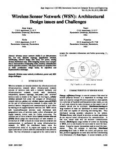
Figure 1. An overview of TriopusNet. The sensor nodes are released from the water inlet points. Each node equips with mechanical arms that can latch to fix a sensor node onto the pipe’s inner surface, thereby controlling node deployment inside the pipeline. Sensor network data is wirelessly transmitted to nearby gateway nodes. dant sensor nodes which increases the deployment cost. TriopusNet shares the autonomic computing concept such that a small number of backup sensor nodes (i.e., equal to the number of expected battery-depleted or faulty sensors) are deposited at a pipeline inlet storage and released on an as-needed basis.
Upon detection of low battery level (or a fault), the sensor node retracts its mechanical arms to detach itself from the pipe’s inner surface. Flow in the pipes carries the battery-depleted sensor node to exit to a pipe outlet. To repair the network disconnection created by the departed sensor node, the TriopusNet system releases a fresh sensor node and runs the sensor replacement algorithm to position the fresh sensor node and adjust the locations of existing sensor nodes to fill any sensing area and repair any network disconnections.
The main contributions of this work are:
Previous research [9] addresses the sensor deployment problem in wireless sensor networks. They formulated this as an optimization problem of how and where to place a minimum number of sensor nodes to achieve the maximum sensing coverage and maintain the best possible network connectivity while consuming the least amount of communication energy. They developed optimizing deployment algorithms to solve this problem. However, previous studies fail to directly address the human effort problem, i.e., human effort is still needed for any in-field sensor deployment (and replacement) at the locations determined by their optimizing deployment algorithms. Though some previous systems [16][15] assume sensor nodes capable of physical mobility, their mobility models are often simulated [16] or require continuously traveling sensor nodes without fixed deployment [15]. TriopusNet complements previous work by leveraging water propulsion to carry sensor nodes from water inlet to scale down human effort, and by creating mobile sensor nodes capable of positioning themselves at locations determined by any optimizing deployment algorithm developed by previous systems.
Different from traditional sensor network deployment in which human effort is needed to place and replace sensors manually, TriopusNet automates sensor deployment and replacement by leveraging natural water propulsion to carry sensor nodes throughout pipes, thus scales down human effort in deploying and maintaining WSN in pipeline monitoring.
This study tests and evaluates TriopusNet by developing a real prototype and pipeline testbed. Results show that automated sensor deployment in TriopusNet successfully produced quality deployment using no more sensor nodes than non-automated static deployment. Results also indicate that automated replacement in TriopusNet successfully replaced a battery-depleted sensor node with a fresh sensor node while recovering data collection rate from the departure of a battery-depleted sensor node.
The rest of this study is organized as follows. Section 2 provides the system overview, assumptions, and limitations. Section 3 describes hardware design. Section 4 presents sensor deployment and replacement algorithms. Section 5 describes the experimental testbed. Section 6 gives experimental results. Section 7 discusses limitations and future extensions. Section 8 reviews related work. Finally, Section 9 concludes the study.
Many related systems [10][19] address fault management in wireless sensor networks. These systems use various techniques to detect sensor node faults and errors, including information fusion for fault detection, collaborative fault detection, etc. However, these techniques do not eliminate the need for human effort to perform in-field replacement of faulty sensor nodes. TriopusNet complements previous work by using free water propulsion to facilitate in-field sensor node replacement. Other previous techniques [17] implement autonomic computing, in which systems self-heal by activating redundant (or backup) components near faulty components. These techniques deploy dense and/or redun-
2. SYSTEM OVERVIEW, ASSUMPTIONS, AND LIMITATIONS To understand system assumptions and limitations, this section first provides an overview of how the system dispatches and places sensor nodes in pipelines (Fig. 1). The pipelines interconnect a set of vertical and horizontal pipes, starting with a single water inlet and ending at multiple water outlets (i.e., faucets). In
62
Figure 2. A TriopusNet node contains (a) gyroscope, (b) water pressure sensors, (c) relays, and (d) Kmote CPU board. The first prototype uses three AAA batteries and three linear actuators. The second prototype uses a lithium battery and one customized motor to drive three arms, resulting in a significant size reduction.
other words, pipelines form a virtual tree in which the inlet is the root node, each faucet outlet is a leaf node, a pipe branch point is an intermediate node, each pipe tube is an edge between parent and child nodes, and each flow path is a downward path from the root node to each leaf node. The inlet also serves as the storage point where sensor nodes are deposited into a dispatch queue at the start of deployment. The TriopusNet releases sensor nodes from the dispatch queue while running the sensor deployment algorithm. This approach forms an interconnected wireless network that covers all possible flow paths with sensors.
3.
Sensor Latching Step: The sensor node continuously computes its current location as it travels through the pipeline. Section 4.4 describes the sensor localization algorithm. When the sensor node approaches its deployment position, it extends mechanical arms to attach itself to the pipe’s inner surface. The sensor node then reports latch completion to the system, and TriopusNet releases the next sensor node (i.e., repeats Step 2). Thus, the deployment of sensor nodes continues until TriopusNet covers all possible flow paths in the pipeline.
The proposed system involves the following four steps.
4.
Sensor Replacement Step: Sensor nodes consume battery power during the data collection phase. At some time point, some sensor node may report low-battery to the system. A low-battery sensor node uses its remaining battery power to retract its mechanical arms and detach itself from the pipe’s inner surface. The sensor node is then carried by the water current to a faucet, where it exits the pipeline. To recover from the sensing area and network disconnection caused by the departed sensor node, TriopusNet releases fresh sensor nodes (from the dispatch queue) during replacement. Section 4.7 describes the sensor replacement algorithm.
1.
2.
Preparation Step: The pipeline spatial topology must be measured a-priori as an input for automated sensor deployment. Interested readers may refer to the PipeProbe system [4] on obtaining pipeline spatial topology. The dispatch queue at the inlet must be filled with sensor nodes ready to be released into the pipeline. Each faucet in the pipeline is turned on, one after another, to create a running flow path from the inlet to each outlet. That is, each faucet must be turned on at least once such that sensor nodes can travel and cover all possible flow paths in the pipelines. Each faucet could be turned on either manually (i.e., by the user) or automatically (i.e., by installing a remote-control actuation device). This preparation step constitutes a onetime manual effort at the start of deployment.
To communicate with sensor nodes inside the pipelines, gateway nodes must be installed prior to any sensor node deployment inside the pipelines. Figure 1 shows that gateway nodes are placed at the inlet and each endpoint in pipelines. To ease manual deployment effort, gateway nodes can be installed outside pipes. To collect data from in-pipe sensor nodes, gateway nodes must have wireless communication with at least one in-pipe sensor node. Gateway nodes must also have a network connection to a laptop (or desktop) computer for remote control, data logging, and automated sensor deployment and replacement algorithms.
Sensor Deployment Step: Prior to releasing each sensor node, TriopusNet runs the sensor deployment algorithm to compute its deployment position. Sections 4.1 and 4.2 describe the sensor deployment algorithm. The system then sends the “release” message including the deployment position, to the head sensor node in the dispatch queue. The head sensor node retracts its mechanical arms from the dispatch tube and starts its pipe journey. Note that the sensor node requires no power for its physical movement as it uses water flow for propulsion.
The following list summarizes TriopusNet’s assumptions (particularly where manual effort is needed) and limitations below:
63
The spatial topology of pipelines must be known, including the pipe length, the pipe’s internal diameter, horizon-
Figure 3. TriopusNet node schematic. An Harrangement of Switch 1 – 4 is used to control the motor.
Figure 4. The final TriopusNet node prototype by Firgelli Technologies [7]. A linear actuator controls a mechanical arm following a linear push and pull motion. To activate a linear actuator for the push motion, the Kmote turns on switch (SW) 1 and 4 to make current flow from left to right on the Hbridge (the right-hand side of Fig. 3). To activate the linear actuator for the pull motion, the Kmote turns on switch (SW) 2 and 3 to reverse the current from flow right to left on the H-bridge. The switches are simply relays controlled by GPIO. To reduce the Triopus node size that is primarily occupied by three PQ-12 linear actuators, the 2nd prototype replaced three motors (each driving a separate mechanical arm) with one motor driving all three mechanical arms and replaced the three AAA batteries with a lithium battery. Motor calibration was achieved by adding a spiral gear that connects and pushes three separate gears moving all three mechanical arms simultaneously. When a Triopus node needs to attach to a pipe location, it extends mechanical arms until they touch the pipe’s inner surface. To ensure that the latching mechanism works well, three arms of a Triopus node point to three different angles and form a triangle. Because pipes have different diameters, the arm’s stroke length must be long enough to touch the pipe’s inner surface on three sides.
tal/vertical turns, and the faucet size. Interested readers may refer to the PipeProbe system [4] on obtaining pipeline spatial topology.
In the absence of automatic faucets, manual effort is required to open each faucet in turn and at least once, such that water runs through all pipelines to ensure complete sensor deployment. In addition, manual effort is required to open each faucet when a battery-depleted or faulty node needs to flow out for replacement. Section 7 discusses how to reduce this manual effort.
The current sensor node measures 6 cm in diameter, which does not fit inside all pipes or may get stuck in some pipes. Given a limited budget in making this proof-of-concept prototype, further engineering efforts may reduce its size. Section 7 discusses how to further reduce the prototype size in the future.
The current sensor prototype uses 2.4 GHz radio (CC2420) to send/receive messages. High frequency radio is not the ideal choice in water, as water absorbs radio waves and limits its transmission range. In water, sonar and light are better communication media than radio [12]. Given this study focuses on the deployment method, we leave the choice of radio an issue to be addressed in the future.
To localize in a vertical pipe segment, a Triopus sensor node measures water pressure using an Intersema MS5541C [21] water pressure sensor. The Intersema MS5541C pressure sensor gives pressure readings within a range of 0 to 14 bars (with a resolution of 1.2 mbars) and consumes less than 5 uA operating current. To detect the horizontal pipe turns, the Triopus sensor node uses a gyro-scope sensor [22] to measure the rotational motion along the yaw (z) axis with a ±300°/s range. The gyroscope sensor module is fixed precisely at the top of the upper half of the node’s hemispheres such that the gyroscope lays flat on the horizontal plane to obtain an accurate z-axis measurement. Figure 4 shows the final prototype of a Triopus Node.
3. HARDWARE DESIGN Figure 2 shows the components of a Triopus node, and figure 3 presents its block diagram and circuit design. The Triopus node consists of (1) a wireless sensor mote called Kmote [6], (2) a motor that drives three mechanical arms for latching onto and delatching from the pipe’s inner surface, (3) a spherical case that encapsulates and waterproofs the node’s electrical components, and (4) pressure and gyroscope sensors used for node localization. The details of these components are described as follows.
4. SYSTEM DESIGN This section describes key software components that support automated sensor deployment and maintenance in TriopusNet. The process of automating sensor deployment and maintenance involves calculating the sensor deployment order, sensor deployment positions, etc. The goal of sensor deployment is two-fold: (1) blockage-free movement and fixation of the sensors in the pipelines, and (2) full sensing and network coverage. The following subsections detail the individual software components as they are activated in the process of a complete deployment and replacement of a battery-depleted node.
The Kmote circuit is a clone of a standard TelosB mote, which features a MSP430 microcontroller and CC2420 radio stack. It is Tiny-OS compatible. The main difference between Kmote and TelosB mote is that Kmote separates the CPU circuit board from the USB program uploader circuit broad. In a field deployment, Kmote needs only the CPU board, thus reducing the form factor size of the Triopus node. The CPU board measures 35 mm (L) x 21 mm (W) x 7 mm and weighs approximately 4 grams. For the latching & delatching mechanism, the first version of Triopus node contains three linear actuators (model PQ-12) made
64
starts the first sensor deployment at the pipe segment p1 (ending at n1) then the pipe segment p2 (ending at n2), and so forth until reaching pipe segment p7. This post-order deployment sequence is important for two reasons. (1) It assures that sensor deployment covers all pipe segments. (2) It orders the deployment of a downstream sensor to precede the deployment of its upstream sensors. This prevents a newly released sensor from traveling past one or more latched sensors that may cause knocking-off or blocking in narrow pipes.
4.2 Sensor Deployment Before sensor nodes can be released, the sensor deployment algorithm computes first the coarse-grain positions – the pipe segment and the approximate latching point. This computation process ensures satisfactory sensing coverage. A Triopus node’s capabilities can be modeled as a coverage function of radio distance and sensing quality. A sensing quality utility function can thus be defined based on the sensor capability or application requirement. This study uses a simple coverage function in which each sensor monitors a disk area with a sensing range (radius) R. In this study, full sensing coverage over the monitored pipelines requires any pipe distance between two neighbor sensors to be less than or equal to 2*R. Sensing coverage means that the sensor network is able to monitor the health of the pipelines in full. Note that this sensor deployment algorithm is not limited to a simple sensor coverage function, but can perform other sensor coverage functions as well.
(a)
Assume that the new sensor node is placed in segment S and the sensing range is R. Subtracting 2*R distance from the most recently deployed sensor node in segment S gives the position of the new sensor node. If segment S is not long enough to accommodate the new sensor node, the new sensor node is placed in the next segment on the sensor deployment order sequence (Sec 4.1). To bootstrap for the leaf segments, the gateway node at the faucet is considered the only node at the beginning. For intermediate segments, i.e., segments with multiple downstream branches, the first sensor node in an intermediate segment is placed at the position such that the distances to all immediate downstream nodes are less than or equal to 2*R.
4.3 Sensor Movement Because sensor mobility leverages the force of water flow within the pipe, an endpoint faucet must be turned on to generate a running flow path. The sensor movement algorithm computes first the flow paths from the inlet to each outlet. The algorithm then selects a path intersecting the pipe segment the node is positioned to. Consider the example in Fig. 5(b). A sensor deployment at the pipe segment p3 requires the running flow path (root → n7 → n6 → n4 → n3) to power its movement. Turning on the endpoint faucet n3 and turning off all other faucets create this flow path.
(b) Figure 5. An example pipeline structure (a) with the corresponding virtual tree (b).
4.1 Sensor Deployment Order This initial phase determines the deployment order of the sensor nodes. Placing nodes close to the releasing point early may result in blockage and hinder the movement of nodes destined for downstream positions. To avoid this problem, the sensor deployment algorithm first transforms the physical layout of the pipelines into a virtual tree, in which the inlet is the root node, each endpoint is a leaf node, each pipe branch point is an intermediate node, and each pipe segment is an edge between parent and child nodes. Figure 5(b) shows the resulting virtual tree transformed from the physical layout (Fig. 5(a)).
4.4 Sensor Localization As a sensor node travels along its flow path, it continuously calculates and updates its location so that it knows when it has arrived at its assigned location. This study adopts the pipeline localization technique from the PipeProbe system [4], which uses a combination of pressure and gyroscope sensors to detect vertical and horizontal pipe turns. As pipelines have many segments, a flowing sensor node can track its location by counting the number of turns encountered on the flow path between the root inlet and the leaf faucet. To determine the segment offset distance from the last turn, the algorithm infers vertical distance offset from the change in water pressure and horizontal distance offset by multiplying node velocity by the traveled time. Since the sensor node was designed
The algorithm subsequently runs a post-order traversal of the virtual tree, in which the resulting node traversal sequence is also the order of node deployment in pipe segments. Consider the example in Figure 5(b). The post-order traversal sequence is {n1, n2, n3, n4, n5, n6, n7}. Following that traversal order, the algorithm
65
sensor nodes over other segments until it reaches full sensing and network coverage.
4.6 Data Collection Upon completion of the sensor deployment, TriopusNet enters the data collection phase and runs the collection tree protocol (CTP) [5] implemented in TinyOS 2.1. To balance the load over its network traffic, this study uses the support for anycast to multiple sinks provided by CTP. In the pipeline scenario, each gateway node acts as a sink for data collection. To reduce the hop count and packet loss rate, a sensor node forwards packets to the gateway node with the least CTP routing cost. Previous study in tunnel monitoring [11] shows that multi-sink collection trees work effectively in node deployments with linear topology.
4.7 Sensor Replacement Figure 6. Pipeline Testbed
Each sensor node continues to monitor its battery level and network connectivity while the system collects pipeline health data. Network connectivity can break as the node battery runs low. This issue is particularly disruptive due to TriopusNet’s tree-like connectivity. A single node failure in such a network can easily result in network partitions, i.e., persistent data losses. Therefore, the system must be able to recover when the battery of a sensor node runs out. The replacement mechanism requires collaboration between the battery-depleted node and good nodes. First of all, the batterydepleted node informs the downstream gateway at the endpoint, so the faucet can be turned on to allow node movement. The battery-depleted node retracts its mechanical arms to flow to an endpoint for node retrieval. At the same time, the battery-depleted node’s downstream nodes are also flushed out to prevent clogging inside the pipeline. This is due to the size of the current prototype being too big for a node to pass through its downstream nodes. For the node retrieval method, we adopt a similar approach from the SmartBall commercial product [23]. A fishing net with a tail is inserted at the ends of pipelines to catch any outgoing sensor nodes. Therefore, a sensor node will not remain inside the pipe when its battery dies.
Figure 7. The lengths (cm) of testbed and 4 test scenarios with its weight density equal to the water density, the node’s flow velocity approximates the water flow velocity.
4.5 Sensor Latching When a sensor arrives at its assigned location, it latches onto the pipe’s inner surface and turns on its radio to listen to beacon packets from downstream sensor nodes or gateway node. The sensor node measures the packet received rate for the link quality. Stable link quality is important because a single link failure may lead to a network partition in a tree-based network topology. Upon detecting a low packet received rate, the sensor node moves one increment closer to its downstream sensor node. This sensor downstream movement requires unlatching from the pipe inner surface, moving forward for t seconds, and re-latching onto the pipe’s inner surface. The sensor node repeats this latching step until a pre-defined link quality threshold is met.
Flushing out the battery-depleted sensor node and its downstream nodes produces an uncovered monitoring area in the system. To repair this uncovered area, each upstream node unlatches itself from the pipe sequentially and flows downstream to find the gateway node or its downstream neighbor node. Each sensor node repeats the process of detachment, movement, localization, and reattachment until the uncovered area reaches the root location. The system then releases fresh nodes from the dispatch queue to cover the remaining area. With a smaller prototype in the future, it is possible that the Triopus node can pass through any upstream and downstream nodes. Therefore, the new node can replace the battery-depleted node without having to move the entire set of nodes in the network. Section 7 discusses how to further reduce the prototype size in the future.
A tricky case is to ensure the first sensor node of an intermediate segment is connected to the sensor nodes of all downstream segments. This sensor node moves downstream until all immediate downstream sensor nodes from all branches are reachable. If a sensor node arrives at the exact branching point but is still unable to reach all downstream sensor nodes, the sensor node moves into one of the unreachable downstream segment until it connects to a sensor node in that segment.
To determine battery depletion, a sensor node simply uses its battery voltage to estimate residual energy and sets a low-battery threshold that triggers node replacement.
Upon successful attachment to a pipe location, the sensor node sends a “latching completion” packet to the system, including its latching position. The system continues to re-lease and deploy
66
Table 1. Results for automated sensor deployment
Scenarios
# of test runs
1
5
Node-to-node coverage distance (cm)
# of node deployed
Mean
TriopusNet
193.7
Std. 65.1
3.6
Static 7
Data collection rate (%)
Positional error (cm)
Time to deployment (sec)
# of latching per node
97.6
6.1
103.7
2.3
2
5
156.8
35.4
4
7
98.4
8.0
117.5
1.6
3
5
166.3
45.4
4
4
98.7
7.94
139.1
2
4
5
173.4
69.3
6
12
98.8
12.6
185.9
2.2
Overall
20
172.7
58.0
4.35
7.5
98.4
9.22
136.5
2.1
5. EXPERIMENTAL DESIGN This section describes the experimental testbed, procedure, and performance metrics.
5.1 Experimental Testbed Figure 6 shows the pipeline testbed used to evaluate performance of TriopusNet. This testbed connects 6 transparent pipe tubes and 2 water valves and forms a pipeline network that starts with one vertical path, followed by a horizontal path, and forks into two paths in the middle of horizontal path. These 6 transparent pipe tubes, each measuring 10 cm in diameter, enable direct observation of how well the sensor nodes flow and latch/de-latch inside the pipes. The two valves at the end of each horizontal path control the volumetric flow rate on each flow path. Figure 7 lists the lengths of each pipe tube segment in the testbed.
5.2 Performance Metrics The following list defines the metrics used to evaluate the performance of TriopusNet.
Data collection rate: This measures the percentage of data packets successfully received by the gateway nodes compared to all packets sent from sensor nodes. Coverage distance: This measures the total pipeline length covered by the deployed nodes. Number of nodes deployed: This counts the number of nodes deployed to cover a given sensing area. Time to deployment: This measures the time to complete the node deployment for a test scenario. Time to replacement: This measures the time to replace a battery-depleted node. Energy Consumption: This measures the energy to complete the node deployment for a test scenario or to replace a battery-depleted node.
Figure 8. Real node locations of three test runs from Scenario 4. It shows the dynamic of each deployment.
to create a running flow path is manual. For the single-outlet scenarios (#1, #2, and #3), the target faucet was turned on to create a flow path before starting the node deployment. In the multi-outlet scenario (#4), each of two faucets was turned on to create two different flow paths for node deployment. (3) After the system deployed all nodes in the pipes, data collection was performed by running the multi-sink collection tree protocol (CTP). During data collection, sensor nodes transmitted data packets back to the gateway nodes/sinks. The gateway is a laptop computer wired to Kmote. Data was logged during both node deployment and data collection for performance analysis.
5.3 Experimental Procedure
To measure sensor node replacement performance, scenario #4 began from a 6-node configuration. Each of the last two downstream sensor nodes was selected in turn by setting its battery level to low. When the test began, the selected node reported a “low-battery level” message and triggered the system’s node replacement. For each low-battery node replacement, we repeated the test 5 times. Over all, there were 10 test runs of node replacement. Each test run involved the following steps. (1) All nodes were restored to their initial configuration. (2) The system started the data collection phase. (3) The selected node reported lowbattery level and triggered node replacement. Data were recorded before, during, and after node replacement for performance analysis.
This study uses four test scenarios in Figure 7 to test TriopusNet’s performance. Each scenario has different pipe area coverage. Scenarios #1, #2, and #3 have the single-outlet sensing areas, and Scenario #4 involves a multi-outlet sensing area. System parameter settings are: the packet received rate (PRR) threshold = 95%, water flow velocity = 12.5 cm/sec, and each node’s sensing range R >= radio range. To measure node deployment performance, each test scenario was repeated five times for a total of 20 (= 4 scenarios * 5 runs per scenario) test runs. The procedure for each test run involved the following steps. (1) All sensor nodes were returned to the water inlet point. (2) In the current testbed, opening and closing a faucet
67
Figure 11. Data collection rate vs. number of transmission hops to gateways.
Figure 9. Coverage distances in L-shape and in I-shape pipe
Figure 10. CDF of data collection rate
Figure 12. CDF of positional errors range for adjacent nodes in the same tube, whereas the L-shape indicates nodes in different tubes. The reason for variation in the radio range is when two adjacent nodes are in different pipe segments (L-shape case), radio signals can travel through air, and therefore travel far. In comparison, for two adjacent nodes within the same pipe segment, radio signals travel mostly in water, which absorbs energy and limits its range. This highlights the benefits of using an online sensor deployment algorithm over a static sensor deployment. In comparison to the static deployment which on average uses 7.5 nodes for deployment, TriopusNet uses only 4.35 nodes.
6. EXPERIMENTAL RESULTS This section describes the results collected from test runs in the experimental testbed.
6.1 Results for Automated Sensor Deployment Table 1 shows the results collected from 20 test runs of automated sensor deployment. To evaluate the quality and efficiency of the automated sensor deployment, this study first shows the node locations and then measures the coverage distance, the number of nodes deployed, the data collection rate, the node’s positional error, the time to deployment, and energy overhead from mechanical latching.
6.1.2 Data Collection Rate (DCR) To quantitatively evaluate whether a network is well connected, this study measures the ratio of data being successfully collected at the gateway. In each test run of each scenario, each sensor node sent 1000 data packets to a gateway node. In other words, if a scenario involved 5 sensor nodes, a total of 5000 data packets were sent from all sensor nodes. Based on four scenarios and 20 test runs, this study logs the ratio of successfully received packets at the gateway nodes over all transmitted packets from each individual node. Figure 10 depicts the cumulative density function (CDF): 80% of the sensor nodes show a data collection rate exceeding 99%, and all sensor nodes have a data collection rate higher than 86.5%.
6.1.1 Node Locations Figure 8 shows the locations of deployed nodes in three test runs (labeled A, B and C) in Scenario #4. This figure also draws the node locations of a static deployment, where nodes are fixed 90 cm apart. This 90 cm measurement is based on repeated measurements for an average radio range between two sensor nodes in a straight pipe. Static deployment is a good baseline for performance comparison because it is the most commonly-used method in sensor deployment. It might have better data collection ratio, but it would need a lot more redundant nodes to hop the data.
The data collection rate varies depending on how far the sensor node is from the gateway. Figure 11 plots the average data collection rate for nodes with different transmission hop counts to the gateway node. This figure also plots the lower-bound data collection rate assuming an exact 95% data collection rate (DCR) for every hop. This can be calculated by taking the n-th power of the DCR threshold in the sensor deployment algorithm, where n is the transmission hop count to reach a gateway node. Note that the sensor nodes only latch when the measured per-hop DCR exceeds the threshold. This result also supports that the latching is reliable
In the TriopusNet system, each test run produces different node locations. The average node-to-node distance over all scenarios is 172.7 cm, with a standard deviation of 58 cm. This large variation implies that the radio range varies significantly from location to location. Examining the dataset reveals that the average radio range is approximately 90 cm for connecting nodes in the same pipe tube. However, the radio range can reach up to 170 cm for nodes placed in different tubes. Figure 9 provides statistics supporting this observation. The I-shape in this figure indicates radio
68
Table 2. Time to replacement The low battery node
# of test run
2nd last
5
Mean 223.4
Last node
5
152.3
# of latching per node
Transmission hops to inlet
Std. 38.8
2.2
3
24.1
2.3
4
Time to replacement (sec)
6.2.1 Data Collection Rate
Figure 13. CDF of the number of latching for all nodes
The data collection rates of the system before a node reported low-battery level and after the node was replaced were 0.989 and 0.984 respectively. This small difference suggests the effectiveness of the automated replacement. The data collection rate without automated replacement was 0.81. The reasons for the high data loss rate without automated replacement were: (1) In the presence of a network hole or an uncovered area, some sensor nodes selected a new route to reach the gateways. These new routes were longer than the original routes, and hence increased the chance of packet losses. (2) In the cases of network partition, isolated nodes reported zero data collection rate.
and the data collection rate does not go below the lower-bound data collection rate.
6.1.3 Positional Accuracy Figure 12 shows the (CDF) of positional errors in each of the 4 scenarios and an assemblage of all scenarios. The dataset for the CDF is based on 18 location estimates of the node in scenario #1, 20 estimates in scenario #2, 20 estimates in scenario #3, and 30 estimates in scenario #4, for a total of 88 location estimates. The overall median error is 7.14 cm, and 90% of the errors are less than 20.45 cm. Node positional accuracy is important for achieving sensing coverage in node deployment, as sensing range and coverage are calculated from node locations. From a practical viewpoint, this positional accuracy is sufficient for most pipeline applications, such as pinpointing the location of pipe leakage.
6.2.2 Time to Replacement The time to recover from a battery-depleted node depends on the location of the node and the size of the network. If the node is far from the root node, the system must repeat the cycle of detecting an uncovered area and then progressively shifting each upstream node to fill a moving area toward the root node. Table 2 shows the average time to replacement. Note that replacing the 2nd last node requires flushing and replacing its downstream node (i.e., the last node). As a result, replacing the 2nd last node has a longer average time to replacement than replacing the last node.
6.1.4 Time to Deployment Table 1 summarizes the average time required to fully deploy nodes in each of the four scenarios. Note that the deployment time excludes the time required for humans to manually turn on/off faucets, because these steps could be automated in the future. If the flow velocity is set at 12.5 cm/sec, the average time to deploy nodes is less than 2.5 minutes.
7. DISCUSSION The prototype evaluation in this study demonstrates the feasibility of the TriopusNet system. However, there are several assumptions and limitations that require future extensions before practical infield deployment.
6.1.5 Energy Consumption The primary energy consumer in the sensor node is in the motor and relays that drive the three mechanical arms. To quantify the energy spent on the mechanical motor and relays, the energy consumed by a single act of latching was measured first. This step consumes 1.01W and takes two seconds, which is less than 1% of the overall energy budget given a 3.7V Polymer Lithium Ion Battery at 600mAh. Subsequently, the number of latching processes required to fix a node deployment was measured (e.g., this may involve repeating the data collection rate measurement and node movement as described in Section 4.5). In total, data were collected from deploying 88 nodes over 20 test runs in four scenarios. Figure 13 shows the CDF on the numbers of required latching per node deployment. The average is 2.35 (latching), whereas 90% of nodes required less than 5 (latching).
The size of the current TriopusNet node prototype is too big to be flushed out independently in small-diameter pipes. In the experiment, when a battery-depleted node detaches from the pipes, its downstream nodes must be flushed out first such that the batterydepleted node does not get clogged by any downstream nodes in the pipe. Flushing good downstream nodes can be prevented by further minimizing the node size such that the battery-depleted node can easily pass through any downstream nodes without clogging the pipes. In addition, the upstream nodes do not have to move downstream for network coverage hole repair because the new node would be able to flow directly to the coverage hole to fix the network disconnection without being blocked by nodes already inside the pipeline. It would also benefit the time to replacement in section 6.2.2. For example, in our current testbed, the time for a node to travel from inlet to outlet is 44 seconds on average. In other word, it means that to replace a battery-depleted node only require 44 seconds at most. Reducing the node size is possible with current micro-mechanical design, particularly on folding the mechanical arms that occupy majority of the space in a sensor node.
6.2 Results for Automated Sensor Replacement Scenario #4 was selected to determine the effects of automated sensor replacement, as it is the most representative scenario among the four scenarios. Each of the last two downstream nodes was set to low battery to trigger automated node replacement five times. The resulting data was then measured to determine the data collection rate and time to replacement.
Since the mobility of TriopusNet node relies on water flow in pipes, node placement requires controlling or obtaining the direction of the water flow in the pipes. In our experiment, we manually
69
turn on one water outlet at a time, so each released node flows on the path leading to its assigned pipe location. Removing this manual effort is possible with automatic touch-free faucets. By attaching a sensor-trigger node to activate/deactivate the infrared sensor in each automatic faucet, the TriopusNet gateway controls each faucet by sending signals to the sensor-trigger node.
calization algorithm needs to obtain the water flow rate at each pipe to compute the location of Triopus node. The NAWNS project’s method can be used to calculate the water flow rate.
We envision an opportunistic node placement scheme in which each deployed sensor node is equipped with a water flow sensor. By gathering water flow information from all deployed nodes inside pipes, the system can infer the current flow path. The system opportunistically releases new nodes whose destinations must match the current water flow path.
The HydroSense system senses and recognizes the unique “water hammer” pressure fingerprint produced by each water fixture. By training and recognizing individual fixture’s fingerprint, the system can accurately infer which water fixture is turned on or off. The idea of single-point sensing also eliminates the human cost of a sensing system. However, HydroSense does not focus on sensor network deployment, whereas TriopusNet aims to reduce human effort in deploying a network.
HydroSense [3] proposes a novel single-point sensing technique that identifies the water usage activities of each water outlet using a single pressure sensor installed at one point within a building.
8. RELATED WORK Related research can be categorized into 2 classes: (1) mobile WSN deployment and (2) WSN in pipeline monitoring.
The PipeProbe project [4] developed a mobile sensor node for determining the spatial topology of hidden water pipelines behind walls. It works by dropping a tiny sensor capsule into pipeline. As this capsule traverses the pipeline, it collects water pressure and gyroscope readings to determine the 3D spatial pipeline layout. The proposed system assumes the pipeline layout is known. Thus, PipeProbe can be used first to discover the pipeline layout if such information is not available.
8.1 Mobile WSN Deployment Deployment has been a notorious issue in successful sensor network application. Previous research [8] provides a guideline for successful sensor network deployment. The human effort involved in installing and maintaining sensors is a tremedous cost, especially in remote on-site field deployment. There have been related systems that automate sensor deployment. For examples, Liu et al. [20] developed a breadcrumb system that leverages the mobility of a firefighter to deploy sensors in an environment. A firefighter carries a lightweight dispenser device that automatically drops and releases sensor nodes along a firefighter’s path. These dropped sensors automatically form a WSN and localize the fireflighter without human attention and effort.
9. CONCLUSION This study presents TriopusNet, a mobile wireless sensor network system for autonomous sensor deployment in pipeline monitoring. TriopusNet scales down human effort in deploying and maintaining WSN infrastructure inside pipes. To show the benefits and feasibility of TriopusNet, we have prototyped and tested the system in a real pipeline testbed. Experimental results have demonstrated that automated sensor deployment was able to produce quality node placement using no more nodes than nonautomated static sensor deployment. Results have also demonstrated that automated sensor replacement was able to successfully restore sensing and network coverage from the departure of a battery-depleted node. We believe that TriopusNet provides an alternative and promising strategy to automate sensor deployment and replacement in pipeline monitoring.
Purohit et al. developed the SensorFly system [18], which is a controlled-mobile aerial sensor network platform for indoor emergency response. When SensorFly is deployed, the nodes perform collaberative localization during flying, which is similar to the deployment algorithm in Section 4. Unlike the current project, SensorFly mobility relies on a battery to power the helicopter-like device, whereas the proposed Triopus node mobility relies on water flow. A Triopus node only consumes energy when it performs latching and delatching tasks.
10. ACKNOWLEDGMENTS
8.2 Wireless Sensor Network for Pipeline Monitoring
We would like to thank our shepherd Gian Pietro Picco and the anonymous reviewers for their insightful comments to improve the quality of this paper.
Recent projects involving WSN technologies for monitoring water pipelines include the PipeNet project [1], the NAWMS project [2], the HydroSense project [3], and the PipeProbe project [4].
11. REFERENCES
The PipeNet project [1] detects, localizes, and quantifies leaks and bursts in water pipelines. PipeNet attaches a variety of acoustic, vibration, pressure, and flow sensors to wireless sensor nodes mounted on pipelines, externally and internally, to detect faults and anomalies. The signals received from these sensor nodes are analyzed to identify and locate leaks. In PipeNet’s deployment, human effort is required to install and repair each sensor node onsite. In contrast, the proposed TriopusNet releasing method eliminates these human efforts to install and maintain sensors in the pipes.
[1] I. Stoianov, L. Nachman, S. Madden and T. Tokmouline. PIPENET: A Wireless Sensor network for pipeline monitoring. In IPSN, 2007. [2] Y. Kim, T. Schmid, Z. M. Charbiwala, J. Friedman and M. B. Srivastava. NAWMS: Non-Intrusive Autonomous Water Monitoring System. In SenSys, 2008. [3] J. Froehlich, E. Larson, T. Campbell, C. Haggerty, J. Fogarty, and S. Patel. HydroSense: Infrastructure- Mediated Single-Point Sensing of Whole-Home Water Activity. In Ubicomp, 2009. [4] T. S. Lai, Y. H. Chen, P. Huang and H. H. Chu. PipeProbe: A Mobile Sensor Droplet for Mapping Hidden Pipeline. In SenSys, 2010. [5] O. Gnawali, R. Fonseca, K. Jamieson, D. Moss and P. Levis. Collection Tree Protocol. In SenSys, 2009. [6] Kmote, INTECH http://www.tinyosmall.com/product_p/100-101.htm
The NAWMS project [2] detects the water outflow rate for each pipe and outlet. This method attaches a vibration (accelerometer) sensor to each pipe to separate the water outflow rate for an individual pipe from the master household water meter. By calibrating and deriving the relationship between the standard deviation of pipe vibration and the mean flow rate in the pipe, the NAWNS system can infer a pipe’s water flow rate from the sensed vibration level produced by each flowing pipe. In TriopusNet, the lo-
70
[15] M. Laibowitz and J. A. Paradiso. Parasitic mobility for pervasive sensor networks. In Pervasive, 2005. [16] K. Dantu, B. Kate, J. Waterman, P. Bailis and M. Welsh. Programming Micro-aerial vehicle swarms with Karma. In SenSys, 2011. [17] T. Bourdenas, M. Sloman and E. C. Lupu. Self-healing for Pervasive Computing Systems. Architecting Dependable Systems VII, Springer-Verlag 2010. [18] A. Purohit, Z. Sun, F. Mokaya and P. Zhang. SensorFly: Controlled-mobile Sensing Platform for Indoor Emergency Response Applications. In IPSN, 2011. [19] S. Guo, Z. Zhong and T. He. FIND: faulty node detection for wireless sensor networks. In SenSys, 2009. [20] H. Liu, J. Li, Z. Xie, S. Lin, K. Whitehouse, J. A. Stankovic and D. Siu. Automatic and Robust Breadcrumb System Deployment for Indoor Firefighter Applications. In MobiSys, 2010. [21] MS5541C Pressure Sensor http://www.intersema.ch/products/guide/calibrated/ms5541 [22] The STMicroelectronics LISY300AL gyroscope chip http://www.st.com/stonline/books/pdf/docs/14753.pdf [23] SmartBall, Pure Technologies http://www.puretechltd.com/products/smartball/smartball_lea k_detection.shtml [24] ROBOBEES project http://robobees.seas.harvard.edu
[7] PQ12-P Linear Actuator, Firgelli. http://store.firgelli.com/pq12-p-linear-actuato12.html [8] G. Barrenetxea, F. Ingelrest, G. Schaefer and M. Vetterli. The hitchhiker's guide to successful wireless sensor network deployments. In SenSys, 2008. [9] A. Krause, C. Guestrin, A. Gupta, and J. Kleinberg. Nearoptimal Sensor Placements: Maximizing Information while Minimizing Communication Cost. In IPSN, 2006. [10] K. Ni, N. Ramanathan, M. N. H. Chehade, L. Balzano, S. Nair, S. Zahedi, E. Kohler, G. Pottie, M. Hansen and M. Srivastava. Sensor Network Data Fault Types. ACM Trans. on Sensor Networks, Vol. 5, No. 3, Article 25, May 2009. [11] M. Ceriotti, M. Corra, L. D'Orazio, R. Doriguzzi, D. Facchin, S. T. Guna, G. P. Jesi, R. L. Cigno, L. Mottola, A. L. Murphy, M. Pescalli, G. P. Picco, D. Pregnolato and C. Torghele. Is there light at the ends of the tunnel? Wireless sensor networks for adaptive lighting in road tunnels. In IPSN, 2011. [12] I. Vasilescu, K. Kotay, D. Rus, M. Dunbabin and P. Corke. Data collection, storage, and retrieval with an underwater sensor network. In SenSys, 2005. [13] G. Chen, S. Hanson, D. Blaauw and D. Sylvester. Circuit Design Advances for Wireless Sensing Applications. Proceedings of the IEEE, Vol.98, No.11, pp.1808-1827, Nov. 2010. [14] Y. C. Wang, C. C. Hu and Y. C. Tseng. Efficient Placement and Dispatch of Sensors in a Wireless Sensor Network. IEEE Trans. on Mobile Computing, Vol. 7, No. 2. pp. 262-274, Feb, 2008.
71