[13] David S. Dummit and Richard M. Foote. Abstract Algebra. ... http://www-math.cudenver.edu/â¼spayne/classnotes/topics.pdf. [21] Igor R. Shafarevich.
TRUNCATED QUADRICS AND ELLIPTIC CURVES by Stephen C. Flink B.S., University of Colorado at Denver, 2000 M.S., University of Colorado at Denver, 2004
A thesis submitted to the University of Colorado Denver in partial fulfillment of the requirements for the degree of Doctor of Philosophy Applied Mathematics 2009
This thesis for the Doctor of Philosophy degree by Stephen C. Flink has been approved by
Stanley E. Payne
William E. Cherowitzo
Ellen Gethner
Sylvia A. Hobart
Michael S. Jacobson
Date
Flink, Stephen C. (Ph.D., Applied Mathematics) Truncated Quadrics and Elliptic Curves Thesis directed by Professor Stanley E. Payne
ABSTRACT Let p be an odd prime and let q = pe . Let E be an elliptic quadric in P G(3, q). The quadric E carries the structure of the projective line P G(1, q 2), and the points of E may be put in a one-to-one correspondence with the points of P G(1, q 2) in a manner that preserves the structure of the quadric, in terms of the respective automorphism groups. In this thesis, we consider the geometric properties of the subset E� of E whose points correspond in this way to the nonzero squares in the Galois Field Fq2 . In the course of determining the number of points of E� on certain hyperplanes of P G(3, q), there arise two families of elliptic curves. The Hasse-Weil theorem is invoked to give bounds on the cardinalities of plane intersections with E� . Empirical results for small values of q show that these bounds are the best possible. The theory of elliptic curves over finite fields is used to establish proofs of other properties of the plane sections of E. A substructure H� of the hyperbolic quadric H in P G(3, q) is defined and studied. H� is analogous to and has geometric properties very similar to those of E� . As with our examination of E� , there arise two families of elliptic curves, and
iii
the Hasse-Weil theorem implies bounds on the cardinalities of plane intersections with H� . We find that the two families of curves which arise in the study of H� are identical with the two families of elliptic curves from the study of E� . We call these families of curves E∩E, parameterized by F∗q , and E6∩E, parameterized by Fq \ {0, 1, −1}. Assume now that q is not a power of 3. We show that the set of curves E∩E is symmetric in the sense that the curves in this set with q + 1 + t points are in one-to-one correspondence with the curves in this set with q + 1 − t points. When q ≡ 3 mod 4, the set of curves E6∩E exhibits the same symmetry.
This abstract accurately represents the content of the candidate’s thesis. I recommend its publication.
Signed
Stanley E. Payne
iv
DEDICATION For Greg
ACKNOWLEDGMENT
This thesis would not have been possible without the assistance of the George Galloway trust. I would also like to thank the mathematics faculty at CU Denver for awarding me a Lynn Bateman Memorial Teaching Award for the Fall semester of 2006. Many people have provided encouragement and useful advice. Their influence may have been inadvertent and seemed small at the time and may have come in the course of working together or from offhand conversations. Thank you to John Wilson, Leanne Holder, Mark Miller, Janice Dugger, Art Busch, Oscar Jenkins, Dave Brown, Frank Thraxton, Sandy Barrett, Victoria Naman, Georgia Meginity, Shannon Raptis and Francis Conry. Special thanks to Rob Rostermundt for our many conversations and for being the designated driver after I completed my comprehensive exam. From the distant past, I need to thank Leona Jackson, Bill Blair, Rick Schmidt, James Plastino and Mark Chamberlin. In no particular order, math courses from Dave Wilson, Hugh Bradley, Tom Kammerling, Markus Emsermann, Rich Lundgen, Dave Fisher, Tom Russell, Bill Cherowitzo, Bruce MacMillan, and Brooks Reid have been particularly enlightening. Thanks again to Bruce MacMillan for allowing me to sit in on his Calculus courses during the 2004-05 academic year. I would like to thank the members of my thesis committee for taking the time to examine this work and for their helpful feedback. Thank you in particular to Stan Payne for his guidance in my research. Most of all, I would like to thank Yongxia for her love, support and patience.
CONTENTS Figures . . . . . . . . . . . . . . . . . . . . . . . . . . . . . . . . . . . .
ix
Tables . . . . . . . . . . . . . . . . . . . . . . . . . . . . . . . . . . . . .
x
Chapter 1. Introduction . . . . . . . . . . . . . . . . . . . . . . . . . . . . . . . .
1
2. Two Quadrics in P G(3, q) . . . . . . . . . . . . . . . . . . . . . . . .
8
2.1 Definitions and Preliminaries . . . . . . . . . . . . . . . . . . . . .
8
2.2 An Elliptic Quadric . . . . . . . . . . . . . . . . . . . . . . . . . . .
11
2.3 A Ruled Quadric in P G(3, q) . . . . . . . . . . . . . . . . . . . . .
17
3. The Actions of Two-Point Stabilizers . . . . . . . . . . . . . . . . . .
19
3.1 The Stabilizer of Two Points of E . . . . . . . . . . . . . . . . . . .
19
3.2 Orbits of Planes Under Gl . . . . . . . . . . . . . . . . . . . . . . .
21
3.3 The Group Stabilizing Two Points of H . . . . . . . . . . . . . . .
23
3.4 Point Sets Associated with Squares . . . . . . . . . . . . . . . . . .
28
3.4.1
The Square Points of E . . . . . . . . . . . . . . . . . . . . . . . .
28
3.4.3
The Square Points of H . . . . . . . . . . . . . . . . . . . . . . .
32
4. Truncated Quadrics and Elliptic Curves . . . . . . . . . . . . . . . . .
37
4.1 Point Counts on Planes Meeting E� . . . . . . . . . . . . . . . . . .
37
4.2 Some Background on Elliptic Curves . . . . . . . . . . . . . . . . .
41
4.3 Birational Transformations Between Quartics and Cubics . . . . . .
43
Elliptic Curves From Orbits O∩E� . . . . . . . . . . . . . . . . . .
43
4.3.1
vii
4.3.3
Elliptic Curves From Orbits O6∩E� . . . . . . . . . . . . . . . . . .
47
4.3.4
Elliptic Curves from Orbits O∩H� . . . . . . . . . . . . . . . . . .
48
4.3.5
Elliptic Curves from Orbits O6∩H� . . . . . . . . . . . . . . . . . .
50
4.3.6
Families of Curves . . . . . . . . . . . . . . . . . . . . . . . . . .
51
4.4 Summary of Plane Intersections with Truncated Quadrics . . . . . .
52
4.4.1
Other Plane Orbit Types . . . . . . . . . . . . . . . . . . . . . .
52
4.4.2
Summary of Plane Intersections for Truncated Quadrics . . . . .
53
4.5 Sums of Point Counts . . . . . . . . . . . . . . . . . . . . . . . . .
56
4.6 The Invariant j and Symmetry of Incidences . . . . . . . . . . . . .
58
4.6.1
Admissible Changes of Variables . . . . . . . . . . . . . . . . . .
59
4.6.4
The Invariant j . . . . . . . . . . . . . . . . . . . . . . . . . . . .
61
Appendix A. Additional Results . . . . . . . . . . . . . . . . . . . . . . . . . . . .
66
A.1 q − 1 Elliptic Quadrics Intersecting in 2 Points . . . . . . . . . . . .
66
A.2 Addition on the Curves . . . . . . . . . . . . . . . . . . . . . . . . .
67
B. Tables of Elliptic Curves . . . . . . . . . . . . . . . . . . . . . . . . .
69
B.1 Tables for Elliptic Curves . . . . . . . . . . . . . . . . . . . . . . .
69
C. Programs . . . . . . . . . . . . . . . . . . . . . . . . . . . . . . . . .
98
C.1 C++ Programs . . . . . . . . . . . . . . . . . . . . . . . . . . . . .
98
C.2 Sage Programs . . . . . . . . . . . . . . . . . . . . . . . . . . . . .
104
References . . . . . . . . . . . . . . . . . . . . . . . . . . . . . . . . . . .
105
viii
FIGURES Figure 2.1
Tangent planes to E and the lines l and l⊥ . . . . . . . . . . . . . . .
3.1
A diagram of the elliptic quadric from the point of view of the stabilizer of two points. . . . . . . . . . . . . . . . . . . . . . . . . . .
3.2
15
31
A diagram of the hyperbolic quadric from the point of view of the stabilizer of two points not on any line of the quadric.
ix
. . . . . . .
35
TABLES Table 4.1
Intersection numbers of E� with planes in P∩E for q = 263 . . . . . .
4.2
The number of Fq -rational points on elliptic curves E = EEω∩ for
38
ω ∈ F263 , their j-invariants and multiplicities in E∩E. . . . . . . . . .
65
B.1 Point counts and j-invariants for curves over F3 . . . . . . . . . . .
70
B.2 Point counts and j-invariants for curves over F5 . . . . . . . . . . .
70
B.3 Point counts and j-invariants for curves over F7 . . . . . . . . . . .
70
B.4 Point counts and j-invariants for curves over F11
. . . . . . . . . .
70
B.5 Point counts and j-invariants for curves over F13
. . . . . . . . . .
71
B.6 Point counts and j-invariants for curves over F17
. . . . . . . . . .
71
B.7 Point counts and j-invariants for curves over F19
. . . . . . . . . .
71
B.8 Point counts and j-invariants for curves over F23
. . . . . . . . . .
72
B.9 Point counts and j-invariants for curves over F29
. . . . . . . . . .
72
B.10 Point counts and j-invariants for curves over F31
. . . . . . . . . .
72
B.11 Point counts and j-invariants for curves over F37
. . . . . . . . . .
73
B.12 Point counts and j-invariants for curves over F41
. . . . . . . . . .
73
B.13 Point counts and j-invariants for curves over F43
. . . . . . . . . .
73
B.14 Point counts and j-invariants for curves over F47
. . . . . . . . . .
74
B.15 Point counts and j-invariants for curves over F53
. . . . . . . . . .
74
B.16 Point counts and j-invariants for curves over F59
. . . . . . . . . .
74
x
B.17 Point counts and j-invariants for curves over F61
. . . . . . . . . .
75
B.18 Point counts and j-invariants for curves over F67
. . . . . . . . . .
75
B.19 Point counts and j-invariants for curves over F71
. . . . . . . . . .
76
B.20 Point counts and j-invariants for curves over F73
. . . . . . . . . .
76
B.21 Point counts and j-invariants for curves over F79
. . . . . . . . . .
77
B.22 Point counts and j-invariants for curves over F83
. . . . . . . . . .
77
B.23 Point counts and j-invariants for curves over F89
. . . . . . . . . .
78
B.24 Point counts and j-invariants for curves over F97
. . . . . . . . . .
78
B.25 Point counts and j-invariants for curves over F101 . . . . . . . . . .
79
B.26 Point counts and j-invariants for curves over F103 . . . . . . . . . .
79
B.27 Point counts and j-invariants for curves over F107 . . . . . . . . . .
80
B.28 Point counts and j-invariants for curves over F109 . . . . . . . . . .
80
B.29 Point counts and j-invariants for curves over F113 . . . . . . . . . .
81
B.30 Point counts and j-invariants for curves over F127 . . . . . . . . . .
82
B.31 Point counts and j-invariants for curves over F131 . . . . . . . . . .
83
B.32 Point counts and j-invariants for curves over F137 . . . . . . . . . .
84
B.33 Point counts and j-invariants for curves over F139 . . . . . . . . . .
85
B.34 Point counts and j-invariants for curves over F149 . . . . . . . . . .
86
B.35 Point counts and j-invariants for curves over F151 . . . . . . . . . .
87
B.36 Point counts and j-invariants for curves over F157 . . . . . . . . . .
88
B.37 Point counts and j-invariants for curves over F163 . . . . . . . . . .
89
B.38 Point counts and j-invariants for curves over F167 . . . . . . . . . .
90
B.39 Point counts and j-invariants for curves over F173 . . . . . . . . . .
91
B.40 Point counts and j-invariants for curves over F179 . . . . . . . . . .
92
xi
B.41 Point counts and j-invariants for curves over F181 . . . . . . . . . .
93
B.42 Point counts and j-invariants for curves over F191 . . . . . . . . . .
94
B.43 Point counts and j-invariants for curves over F193 . . . . . . . . . .
95
B.44 Point counts and j-invariants for curves over F197 . . . . . . . . . .
96
B.45 Point counts and j-invariants for curves over F199 . . . . . . . . . .
97
xii
1. Introduction The focus of this dissertation is on a question in three-dimensional projective geometry, P G(3, q), when Fq is an arbitrary finite field of odd order. Our principal problem is to determine geometric properties of an object with a natural algebraic definition, but whose geometric structure is not obvious. We begin with a nondegenerate quadric Q in P G(3, q). We partition the points of Q so that the partite classes correspond in a natural way with the elements of the ˜ q = Fq ∪ {∞}. We study the geometry of Q� , the set of points extended field F associated with the nonzero squares in Fq under this partition. We call Q� a truncated quadric. Our problem is to describe Q� in terms of plane intersections. The first step is to classify all orbits of planes under the action of the group stabilizing our partition. We find that the most interesting orbits fall into two classes for each of the two types of quadric under consideration. Counting points of Q� on planes in these orbits is shown to be equivalent to counting points on certain nonsingular elliptic curves. These are algebraic curves of genus 1, for which there exists a large and rich theory. We apply the Hasse-Weil Theorem, a deep result which gives bounds on the number of points on algebraic curves over finite fields. This theorem, in turn, gives us bounds on the cardinalities of plane intersections with the truncated quadrics. We present numerical results establishing the tightness of these bounds. We give a simple characterization of the families of elliptic curves which arise when considering each type of orbit. Finally, we explain a symmetry of incidence numbers which occurs in certain
1
families of orbits of planes, which have the property that for every plane meeting the truncated quadric in meeting it in
q+1 2
q+1 2
+ t points, there is a plane in the same family
− t points.
In Chapter 2, we recall basic notions from projective geometry over finite fields. We review results which establish that the elliptic quadric is the unique example of an ovoid in P G(3, q) when q is odd. The points of an elliptic quadric in P G(3, q) may be put in one-to-one correspondence with the points of the projective line P G(1, q 2) so that each reflects the structural properties of the other. We point out that this is analogous to the identification of the points of the extended complex plane with the unit sphere via stereographic projection. Choosing a specific elliptic quadric E, we show how to make the correspondence between the points of E and P G(1, q 2) explicit. We find that the norm map from F∗q2 to F∗q partitions the points of E \ {0, ∞} into q − 1 disjoint ovals. This partition is the same as the partition induced by a certain flock of E. Fix the points 0 and ∞ of E, and define the line to be the line of intersection of the tangent planes to E at 0 and ∞. For each of the q − 1 non-tangent planes on l⊥ , we choose representative vectors parameterized by the nonzero elements of Fq . This choice of representatives is such that for each value a ∈ F∗q , the points of E on the plane with representative a are the elements of F∗q2 with norm a. In Section 2.3, we choose a specific hyperbolic quadric H in P G(3, q) whose algebraic form bears a strong resemblance with the form chosen for the elliptic quadric E. In E, the points corresponding to Fq ∪ ∞ form an oval o, and E ∩ H = o. If we remove a certain pair of points from H, the remaining points may be partitioned into q + 1 subsets. In fact, the set of q + 1 planes we used
2
to partition E are used to partition the points of H, in a manner different from but analogous to the partition for E. We find that a subset of the points of H has a natural partition into q − 1 arcs of size q − 1. In Chapter 3, we examine the actions of the stabilizers of the elliptic and hyperbolic quadrics on lines and planes in P G(3, q). Recall our identification of the points of the elliptic quadric E with the points of the projective line ˜ q2 = Fq2 ∪ ∞. We are interested in the action of P G(1, q 2), and so with the set F the group Gl stabilizing the points 0 and ∞ of the quadric, as this is the group stabilizing our partition. In Section 3.2, Theorem 3.2.1 describes the orbits of all planes of P G(3, q) under the action of Gl . In section 3.3, we describe the geometry of the hyperbolic quadric H and the action of the stabilizer Hl of 0 and ∞ in a manner analogous to the work in Sections 3.1 and 3.2 for E. Theorem 3.3.1 describes all orbits of planes under the action of Hl . In section 3.4, we define our truncated quadrics E� and H� . These are the subsets of E and H which correspond to squares in Fq under the respective partitions of the quadrics described in Chapter 2. The truncated elliptic quadric E� is stabilized by Gl� , a group of index 2 in Gl . The truncated hyperbolic quadric H� is stabilized by a group Hl� of index 2 in Hl . Having described the actions of Gl and Hl , it is straightforward to describe the actions of Gl� and Hl� on the planes of P G(3, q). We do so in Theorems 3.4.2 and 3.4.4. For each of the stabilizing groups Gl� and Hl� , there are orbits of planes whose intersections with the truncated quadric are easily described. For example, when q − 1 of the q + 1 planes on a line are all in the same orbit, the planes
3
are known to partition a point set of a certain size (say 12 (q 2 − 1)), and so must each contain 21 (q +1) points of the truncated quadric. Define an interesting orbit of planes (under the action of Gl� or Hl� ) to be one whose intersection numbers with their respective truncated quadric are not immediately obtained by application of the orbit-stabilizer theorem. We find that it is sufficient to consider two ∗ families of interesting orbits for each of the truncated quadrics: {Oω∩ E� : ω ∈ Fq } ∩ ∗ : ω ∈ F∗q \ {2, −2}} for E� and {Oω∩ and {Oω6E� H� : ω ∈ Fq \ {2, −2}}, and ∩ {Oω6H� : ω ∈ F∗q } for H� . These interesting orbits of planes have the property
that no more than two planes in such an orbit meet in the same line. For each family of orbits, we choose a line such that each orbit of planes in the family has 2 representatives in the set of planes on that line. In the remainder of the thesis, we describe the intersection of planes from these classes with our truncated quadrics and examine some of the consequences of that description. In Section 4.1, we offer a summary of results from algebraic geometry in general and from the theory of elliptic curves in particular, which we will use in subsequent proofs. Most important for us is the Hasse-Weil theorem, stated in Theorem 4.2.2, which gives bounds on the number of points on an elliptic curve. Also important is Theorem 4.2.1, which states that every curve is birationally equivalent to a unique nonsingular curve. In Section 4.2, we begin with a plane αω in an interesting orbit Oω∩ E� under Gl� . Some algebra on the equations describing the intersection of αω with E� yields a plane curve CF whose Fq -rational points are in 2:1 proportion with the points of αω ∩ E� . The equation for the curve CF is of the form s2 = g(a), where g is a quartic in x without repeated roots. In Section 4.3, we show that this curve is birationally equivalent to a
4
curve whose equation is of the form y 2 = f (x), where f is a cubic in x without repeated roots. This is a standard form for an elliptic curve, and we may bring to bear upon our problem substantial theoretical machinery. In Theorem 4.3.1, an application of the Hasse-Weil theorem, we find that q−1 √ q−1 √ − q ≤ |αω ∩ E� | ≤ + q. 2 2 In section 4.4, we consider intersections of truncated quadrics with representative planes from our other interesting orbits under Gl� and Hl� . We again obtain elliptic curves from the equations for plane intersections and again apply the Hasse-Weil theorem. Also in Section 4.3, we show that the two families of curves which arise from E� are identical to the two families of curves which arise from H� . In Section 4.4, we use our use results from Sections 4.2 and 4.3 to describe bounds of point counts on planes in other orbits. The idea here is that Gl� stabilizes both E� and E6� = E \ (E� ∪ {0, ∞}), and we are able to find an element ϕ of Gl which interchange E� and E6� . Then ϕ also interchanges αω with a plane with the property that |αω ∩ E� | + |ϕ(αω ) ∩ E� | = q + 1. The situation is again similar for H� . We summarize point counts of plane intersections with the truncated quadrics in Theorems 4.4.3 and 4.4.4. In section 4.5, we explain a property of some of the families of orbits of planes under Gl� . The property occurs for families of interesting orbits whenever q ≡ 3 mod 4 and in certain cases when q ≡ 1 mod 4. Let P be such a family of orbits. Then whenever there is an orbit O ∈ P whose planes meet E� in points, there is a different orbit O′ ∈ P whose planes meet E� in
q+1 2
q+1 2
+t
− t points.
The proof that these planes come in these complementary pairs is accomplished
5
using properties of a numeric invariant of the associate elliptic curves. Appendix A.1 contains a minor result which is not used in the main part of the thesis, but which might be of independent interest. Here we describe a set of q − 1 elliptic quadrics whose pairwise intersection is {0, ∞}, all of which are stabilized by Gl . A description of an analogous family of hyperbolic quadrics whose pairwise intersection is a set of four points of P G(3, q) not all in one plane is given in Section 6.1 of [20]. Appendix B contains tables of elliptic curves for each of the two families described in Theorem 4.4.3, for odd primes q < 200. For a given q and for each of the two families of curves, the table gives the j-invariant of each curve, the number of Fq -rational points on the curve, and the number of times the curve occurs in that family. Appendix C.1 contains a program in C++ written to produce the tables in Appendix B. Appendix C.2 contains a short program in SAGE which uses some built-in elliptic curve functions. This program was written to verify the accuracy of the C++ program in section C.1. The work presented in this thesis originated with an attempt to construct sets of points in P G(n, q) with the property that the cardinalities of hyperplane intersections with the set take on relatively few values. We see from Theorems 4.5.1 and 4.5.2 and from the tables in Appendix B that the truncated quadrics are highly irregular with respect to plane intersections. Let S be a subset of P G(n, q) such that the cardinalities of hyperplane intersections with S take on few values. If these cardinalities take on k values, we call S a k-intersection set. Nondegenerate quadrics provide examples of 2-intersection sets in P G(n, q) when n is odd. Some of our early motivation came from the construction of Brouwer
6
in [2], which yields 2-intersection sets by removing points from nondegenerate quadrics in odd-dimensional projective space. Another important work on 2intersection sets is [4], which lists all such sets known at that time and explains how 2-intersection sets may be used to construct strongly regular graphs and 2-weight codes. The literature on quadrics in finite projective space is large and varied. We acknowledge the influence of several works whose results and terminology did not directly come into play in the final version of this thesis. Elliptic and hyperbolic quadrics give examples of finite circle planes. A standard reference on the circle planes associated with elliptic quadrics is Chapter 6 of [11]. The Ph.D. thesis of Orr [19], as reworked in [20], and the paper [3] by Bruck helped us to find a proper frame of reference and to steer clear of some false conjectures.
7
2. Two Quadrics in P G(3, q) 2.1 Definitions and Preliminaries In this section, we give a brief review of some relevant results from finite projective geometry. We follow Stan Payne’s book [20] for theorems and notation. Much of what we describe here may be found in [7], which is a good introductory text on projective geometry. Let V be a vector space of dimension n + 1, for some 0 < n < ∞ over a field F. The projective geometry P(V ) is the geometry whose r-dimensional subspaces are defined to be the r+1-dimensional subspaces of V , for r = 0, . . . , n. Incidence in P(V ) is defined by subspace containment in V . We call the 0−, 1- and 2-dimensional subspaces of P(V ) the points, lines and planes of the geometry, and an (n − 1)-dimensional subspace is a hyperplane. When F is a field with q elements, we write P G(n, q) to denote P(V ). For our purposes, the term projective plane will refer to P G(2, q), although there exist other examples of projective planes. We refer the reader to the early chapters of [20] and to Chapter 1 of [7] for an axiomatic approach to projective geometry. In P G(n, q), we use a row vector x = (x0 , x1 , . . . , xn ) to represent a point and a column vector π = [y0 , y1 , . . . , yn ]T a hyperplane in P G(n, q), with the understanding that for the vector representing a point or hyperplane, we may substitute any nonzero scalar multiple of that vector. The vector representing π generates the null space of all the points incident with π. That is, the point x is incident with the hyperplane π whenever xπ = 0.
8
When q is the power of an odd prime, lois field Fq are squares and
q−1 2
q−1 2
of the nonzero elements of the Ga-
are nonsquares. We will let � and � 6 respectively
denote the set of nonzero squares and the set of nonsquares in Fq . Throughout the main text of this thesis, we use η to denote a fixed but arbitrary nonsquare in Fq . An oval in a projective plane π of order q is a set of q + 1 points, no three collinear. Let P be a point on an oval o. Of the q + 1 lines through P , q are secant lines, meeting o in exactly one other point. The remaining line through P is the tangent line to o at P . It can be shown that when q is odd, each point of π \ o is on 0 or 2 tangent lines. When q is even, one may show that there is a point N such that all tangent lines to o meet at N. That is, when q is even, an oval may be extended to a hyperoval, a set of q + 2 points, no three on a line. A quadric Q in P G(n, q) is a set of points x = (x0 , x1 , . . . , xn ) satisfying a homogeneous quadratic equation f (x0 , . . . , xn ) =
n X n X
aij xi xj = 0
i=0 j=i
for some aij ∈ Fq not all zero. Let A = (aij ) be the upper triangular matrix such that f (x0 , . . . , xn ) = xAxT , and let B = A+ AT . A point of Q is a singular point provided BxT = 0 and xAxT = 0. We say that the quadric Q is degenerate (or singular) if it has a singular point. In P G(2, q), a nondegenerate quadric is a conic. Every conic is an example of an oval. When q is odd, the converse is true as well. Theorem 2.1.1 (Segre) Every oval in P G(2, q), q odd, is a conic.
9
Our primary interest is in quadrics in P G(3, q). For a point x on a nonsingular quadric Q, define the tangent hyperplane to Q at x to be the hyperplane x⊥ := BxT . It can be shown that in P G(3, q), there are exactly two nonisomorphic nonsingular quadrics. When for all x ∈ Q, x⊥ intersects Q in more than just x, it happens that x⊥ ∩ Q is the union of two lines which meet at x. In this case, Q is a hyperbolic quadric. The quadric Q is an elliptic quadric if for each x ∈ Q, Q ∩ x⊥ = x. In this case, for each point x of Q, every line meeting x and not contained in x⊥ meets Q \ {x} in exactly one point. A set S of points of P G(3, q) is called an ovoid if it satisfies the following: 1. Each line meets S in at most 2 points. 2. Each point of S lies on exactly q + 1 tangent lines, all of which lie on a plane. Let P be a point on an ovoid S. Since P is on exactly q + 1 tangent lines, the remaining q 2 lines through P must meet S in exactly one other point. Thus S has exactly q 2 + 1 points. A k-cap in P G(3, q) is a set K of k points, no three on a line. We can think of k-caps as the convex objects in P G(3, q). We can show that ovoids are examples of maximal k-caps. Lemma 2.1.2 If q is odd and K is a k-cap in P G(3, q), then k ≤ q 2 + 1. Proof:
Let P and Q be points of K and consider a plane π on the line P Q.
We claim that |π ∩ K| ≤ q + 1. The q + 1 lines of π meeting P each meet K in at most one other point, so |π ∩ K| ≤ q + 2. Suppose |π ∩ K| = q + 2. If R
10
is a point of π not on K, then each line in π through R must meet K in 0 or 2 points. But this is not possible, since q + 2 is odd. Thus |π ∩ K| ≤ q + 1. Thus the planes on P Q contain at most (q + 1)(q − 1) + 2 points of K. One may show that every q 2 + 1-cap K has the property that for every point P of K there is a unique plane πP such that πP ∩ K = P . That is, every q 2 + 1-cap is an ovoid. We see from the definition that every elliptic quadric is an ovoid. When q is odd, the converse is true as well. Theorem 2.1.3 (Barlotti, Panella) When q is odd, every ovoid in P G(3, q) is an elliptic quadric. Hence in P G(3, q), q odd, the study of ovoids and of k-caps of maximum size is reduced to the study of elliptic quadrics. Further, all elliptic quadrics in P G(3, q) are projectively equivalent. See Theorem 5.4.4 in [20] for proof of this fact. Thus the study of ovoids is reduced to the study of an essentially unique object for each odd prime power q. 2.2 An Elliptic Quadric Let η be a nonsquare in Fq , q odd, and let
Then
0 1 E= 0 0
1
0
0
0
0 −2 0
0
0
0 . 0 2η
E = {x = (x0 , x1 , x2 , x3 ) : xExT = 0}
11
is an elliptic quadric. An explicit representation of the points is E = {(1, s2 − ηt2 , s, t) : s, t ∈ Fq } ∪ {(0, 1, 0, 0)}. For a point x, the unique tangent plane to E at x is the plane ExT . Using the explicit form, we may define addition and multiplication on the points of E \ {(0, 1, 0, 0)} by (1, s2 –ηt2 , s, t) + (1, u2–ηv 2 , u, v) = (1, (s + u)2 –η(t + v)2 , s + u, t + v) (2.1) and (1, s2 –ηt2 , s, t)(1, u2–ηv 2 , u, v) = (1, (s2 –ηt2 )(u2 –ηv 2), su + ηtv, sv + tu).(2.2) √ Note that {1, η} are a basis for Fq2 over Fq , that is, we may represent Fq2 = √ {s + ηt : s, t ∈ Fq } and it is easy to show that θ : Fq2 → E \ {(0, 1, 0, 0)} θ :s+
√
ηt 7→ (1, s2 − ηt2 , s, t)
is a field isomorphism, using operations defined above. √ √ We claim that η q = − η. The map r 7→ r q on Fq2 is a field automorphism √ √ fixing only Fq ⊆ Fq2 . Then (s2 − ηt2 )q = (s + ηq t)(s − η q t). Thus s2 − ηt2 = √ NFq2 /Fq (s+ ηt), where NFq2 /Fq is the relative norm from Fq2 to Fq . Given a fixed basis for the vector space F2q2 underlying P G(1, q 2), we choose representatives for the points of the projective line so that P G(1, q 2) = {(1, a) : a ∈ Fq2 } ∪ {(0, 1)}. We identify the points of E with the points of P G(1, q 2) by (1, s2 − ηt2 , s, t) ↔ (1, s +
12
√ ηt)
(2.3)
and (0, 1, 0, 0) ↔ (0, 1) = (∞). Note that s2 − ηt2 is a square in Fq if and only if s +
(2.4) √
ηt is a square in F2q .
To see this, let α be a primitive element of Fq2 . Then αq+1 generates F∗q ⊆ F∗q2 . √ √ √ Suppose s + ηt = αn . Then s2 − ηt2 = (s + ηt)(s − ηt) = (αq+1 )n . We will say that a point P = (1, s2 − ηt2 , s, t) of E is square if s2 − ηt2 ∈ � and that P is a nonsquare if s2 − ηt2 ∈ � 6 . We label the points (1, 0, 0, 0) and (0, 1, 0, 0) with 0 and ∞, respectively. Define E� = {(1, s2 − ηt2 , s, t) : s2 − ηt2 ∈ �}
(2.5)
E6� = {(1, s2 − ηt2 , s, t) : s2 − ηt2 ∈ � 6 }
(2.6)
and
To better motivate our definition of E� , consider the sphere Z of radius 1 whose center is at the origin in R3 . Let P = (0, 0, 1) and let Π be the plane z = 0. Define the map taking a point Q = (x, y, z) on Z to the ρ : Z \ {P } → Π � � y x , ,0 . ρ : (x, y, z) 7→ 1−z 1−z This is stereographic projection of Z \ {P } onto the xy plane. If we identify each point (x, y, 0) with the complex number x + yi, we have identified the points of Z \ {P } with the complex numbers. Let P C = {(1, ζ) : ζ ∈ C} ∪ {(0, 1)}
13
be the complex projective line. Then the map ρ : Z \ {P } → P C ρ : (x, y, z) 7→ (1,
x y + i) for z 6= 1 1−z 1−z
ρ : (0, 0, 1) 7→ (0, 1) = ∞
identifies the points of Z with the points of the complex projective line. The unit sphere, so identified with the extended complex numbers C ∪ ∞ is the Riemann sphere. The map ρ is analogous to our identification of the points of E with the projective line P G(1, q 2). Then the set of points Z� = {(x, y, z) ∈ Z \ {P } : z > 0}
(2.7)
is analogous to E� . Although we will not require it later, we may make explicit the correspondence between the points of E \ {∞} and the points of an affine plane. We project from ∞ = (0, 1, 0, 0) through the remaining points of E to the plane π = [0, 1, 0, 0]T . The line h(0, 1, 0, 0), (1, s2 − ηt2 , s, t)i meets π in the point (1, 0, s, t). No points of E are mapped to the line at infinity h(0, 0, 1, 0), (0, 0, 0, 1)i of π. Let l = h(1, 0, 0, 0), (0, 1, 0, 0)i. The tangent planes to E at the points (1, 0, 0, 0) and (0, 1, 0, 0) are [0, 1, 0, 0]T and [1, 0, 0, 0]T respectively, which meet in the line l⊥ = h(0, 0, 0, 1), (0, 0, 1, 0)i. The planes on l⊥ different from the tangents [1, 0, 0, 0]T and [0, 1, 0, 0]T are VE = {πc = [1, −c−1 , 0, 0]T : c ∈ F∗q }
14
(2.8)
[1,0,0,0]T
[0,1,0,0]T l⊥
(1,1,−1,0) (1,s2 ,−s,0) m l (1,0,0,0)
(1,s2 ,s,0)
(0,1,0,0)
(1,1,1,0)
m′ (1,η,−1,0)
(1,η,1,0) (0,0,1,0)
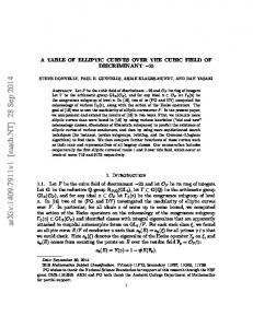
Figure 2.1: Tangent planes to E and to at the points (1, 0, 0, 0) and (0, 1, 0, 0) are the planes [0, 1, 0, 0]T and [1, 0, 0, 0]T , respectively. The oval o = {(1, s2, s, 0) : s ∈ Fq } ∪ {(0, 1, 0, 0)} in the plane [0, 0, 0, 1]T is the intersection of our chosen elliptic quadric E with our chosen hyperbolic quadric H. The lines l and l⊥ are both fixed by Gl . The planes in VE all meet in the line l⊥ and the planes in FE all meet in l.
15
each of which meets E in the oval {(1, s2 − ηt2 , s, t) : s2 − ηt2 = c}. This implies that for c ∈ F∗q , there are q + 1 pairs (u, v) such that u2 − ηv 2 = c. For future reference, define VE� = {[1, −c−1 , 0, 0]T : c ∈ �} and VE6� = {[1, −c−1 , 0, 0]T : c ∈ � 6 }. The planes on l are FE = {αa = [0, 0, 1, a]T : a ∈ Fq } ∪ {α∞ = [0, 0, 0, 1]T }. The plane α∞ meets E in the oval o = {(1, s2 , s, 0) : s ∈ Fq } ∪ {(0, 1, 0, 0)}
(2.9)
and for the remaining planes in FE, αa ∩ E = {(1, s2 − ηt2 , s, t) : s = −ta} ∪ {(0, 1, 0, 0)}.
(2.10)
Note that if (−ta)2 − ηt2 = r 2 then (−vta)2 − η(vt)2 = (vr)2 and that both (1, (−ta)2 − ηt2 , −ta, t) and (1, (−vta)2 − η(vt)2 , −vta, vt) are on αa . It follows that, for b ∈ Fq , the points of E \ {(1, 0, 0, 0), (0, 1, 0, 0)} on αb are either all square or all nonsquare. As with VE, define a partition of FE by FE� = {αa : αa ∩ E� 6= ∅} and FE6� = {αa : αa ∩ E6� 6= ∅}. We refer to Figure 2.1 for a schematic of the relationship between the points of E, VE, and FE. 2.3 A Ruled Quadric in P G(3, q)
16
We describe a particular hyperbolic quadric H in P G(3, q), with an emphasis on the geometric similarities H has with E. For a more complete description of hyperbolic quadrics in P G(3, q), we refer to sections 6.1 and 6.2 of [20]. Put
and let
0
1 H= 0 0
1
0
0
0
0 −2 0
0
0
0 0 2
H = {x : xHxT = 0} = {x : x0 x1 − x22 + x23 = 0} The points may be described explicitly: H = {(1, s2 − t2 , s, t) : s, t ∈ Fq } ∪ {(0, 1, s, s) : s ∈ F∗q } ∪{(0, 1, s, −s) : s ∈ F∗q } ∪{(0, 0, 1, 1), (0, 0, 1, −1), (0, 1, 0, 0)}. H contains the oval o = {(1, s2, s, 0) : s ∈ Fq } ∪ {(0, 1, 0, 0)} in the plane [0, 0, 0, 1]T , in common with E and indeed H∩E = o. Let l = h(1, 0, 0, 0), (0, 1, 0, 0)i as in our description of E. The line l⊥ = h(0, 0, 1, 0), (0, 0, 0, 1)i meets H in the points (0, 0, 1, 1) and (0, 0, 1, −1), and the planes [1, 0, 0, 0]T and [0, 1, 0, 0]T on l⊥ are tangent at the points (1, 0, 0, 0) and (0, 1, 0, 0) respectively. The remaining planes on l⊥ are VH = {πc = [1, −c−1 , 0, 0]T : c ∈ Fq }, each of which meet H in the q + 1 points of an oval. In particular, H ∩ πc = {(1, s2 − t2 , s, t) : s2 − t2 = c} ∪ {(0, 0, 1, 1), (0, 0, 1, −1)}. (2.11)
17
Let P be a point of H that is not on [1, 0, 0, 0]T or [0, 1, 0, 0]T . Then P has the form (1, a2 − b2 , a, b) for some a, b ∈ Fq , a 6= ±b. We say that P is square if a2 − b2 ∈ �, and nonsquare if a2 − b2 ∈ � 6 . Now define partitions of VH and FH by VH� = {[1, −c−1 , 0, 0]T : c ∈ �} and VH6� = {[1, −c−1 , 0, 0]T : c ∈ � 6 }. and FH� = {αa : αa ∩ H� 6= ∅} and FH6� = {αa : αa ∩ H6� 6= ∅}. Then the square points of H are all on the planes of VH� and are all on the planes of FH� and the nonsquare points of H are all on the planes of VH6� and are all on the planes of FH6� . The reasoning is the same as with that for E in the previous section.
18
3. The Actions of Two-Point Stabilizers In this chapter, we will determine the actions of the stabilizers of the truncated quadrics E� and H� on the planes of P G(3, q). This will reduce our problem of finding cardinalities of plane intersections with the quadrics to one involving relatively few orbit types. 3.1 The Stabilizer of Two Points of E In section 6.4 of [20], the stabilizer in GL(4, q) of the elliptic quadric E is found to be the group G generated by 2 2 1 a − ηb 0 1 {[τa,b ]} = 2a 0 0 −2ηb {[ϕa,b ]} =
1
0
0
0 a2 − ηb2 0 0
0
a
0
0
ηb
0 1 N = 0 0
1
0
0
0
0
1
0
0
a 0 1 0
b
0 : a, b ∈ Fq 0 1
0 0 : a, b ∈ Fq , (a, b) 6= (0, 0) , b a
1 0 0 M = 0 0 0 1 0
19
0 1 0 0
0
0
0 0 . 1 0 0 −1
Recall the identification of the points of E with the points of P G(1, q 2) given in equations 2.3 and 2.4. We note simply that the set {[τa,b ]} is a group isomorphic to the additive group of Fq2 fixing (0, 1, 0, 0) = (∞), and {[ϕa,b ]} is a group isomorphic to the multiplicative group of Fq2 fixing (1, 0, 0, 0) = 0 and (0, 1, 0, 0). The element N interchanges 0 and (∞), and it is easy to show that G is 3transitive on the points of E. It is possible to show that G′ , the commutator subgroup of G is isomorphic to P SL(2, q 2). We refer to Chapter 12 of [24] for details. Henceforth, we drop the brackets and write ϕa,b for the matrix [ϕa,b ]. The stabilizer of the pair of points {(1, 0, 0, 0), (0, 1, 0, 0)} is the group Gl generated by M, N and {ϕa,b }. Note that the points of E\{(1, 0, 0, 0), (0, 1, 0, 0)} are the nonzero elements of Fq2 under the isomorphism θ. The group G stabilizing the elliptic quadric contains P SL(2, q 2) as a subgroup. See p. 190 of [24] for a proof. Observe that {ϕa,b } and M{ϕa,b }M form distinct subgroups of Gl , each of order q 2 − 1 and which intersect in {ϕa,b : a2 − ηb2 = 1}, a subgroup of order q + 1. Thus h{ϕa,b }, M{ϕa,b }Mi is a group of order
(q 2 −1)2 q+1
= (q + 1)(q − 1)2 .
The element N normalizes h{ϕa,b }, M{ϕs,t }Mi and thus Gl is a group of order 2(q + 1)(q − 1)2 . Note that A = {a2 I : a ∈ F∗q } is a subgroup of Gl fixing all points. Consider the line m = h(1, 1, 1, 0), (1, 1, −1, 0)i secant to E.
The element ϕs,t takes m to h(1, s2 − ηt2 , s, t), (1, s2 − ηt2 , −s, −t)i, so
the orbit of m under Gl has order at least
q 2 −1 . 2
On the other hand, m
is stabilized by Gm = hM, N, A, ϕ−1,0 i ≤ Gl , a group of order 4(q − 1), so {{(1, s2 − ηt2 , s, t), (1, s2 − ηt2 , −s, −t)} : (s, t) 6= (0, 0)} constitutes the entire
20
orbit of {(1, 1, 1, 0), (1, 1, −1, 0)}, under the action of Gl . Similarly, we see that the line m′ = h(1, η, 1, 0), (1, η, −1, 0)i is exterior to E and is in an orbit of size
q 2 −1 2
under Gl .
3.2 Orbits of Planes Under Gl Let L∩E be the set of lines in the orbit of m under Gl and let L6∩E be the orbit of m′ under Gl . Choose ω 6= 0 and consider the plane [1, −1, 0, ω]T containing m. It is easy to check that under the stabilizer in Gl of m, the orbit of [1, −1, 0, ω]T is {[1, −1, 0, ±ω]T }, and that the orbit under the action of the stabilizer of m′ of [1, −η −1 , 0, ω]T is {[1, −η −1 , 0, ±ω]}. Define TE to be the set of lines generated by one of (1, 0, 0, 0), (0, 1, 0, 0) and a point of l⊥ . It is straightforward to show that Gl acts transitively on the points of l⊥ , and that l⊥ is fixed by Gl . Because N ∈ Gl interchanges (1, 0, 0, 0) and (0, 1, 0, 0), it follows that TE is a single orbit of lines under Gl . Theorem 3.2.1 The orbits of planes of P G(3, q) under the action of Gl , the stabilizer of {(1, 0, 0, 0), (0, 1, 0, 0)} are as follows: 1. The two tangent planes [0, 1, 0, 0]T and [1, 0, 0, 0]T to E at (1, 0, 0, 0) and (0, 1, 0, 0), respectively. 2. The set of q 2 − 1 planes tangent to E \ {(1, 0, 0, 0), (0, 1, 0, 0)}. 3. The q − 1 planes VE = {πc = [1, −c−1 , 0, 0]T : c ∈ F∗q }. 4. The q + 1 planes FE = {γa,b = [0, 0, a, b]T : a, b ∈ Fq }1 . 1
We shall see that this is a useful way to represent these planes
21
5. The planes not tangent to E and meeting E in exactly one of (1, 0, 0, 0), (0, 1, 0, 0) form an orbit of size 2(q 2 − 1). These are the planes which are not tangent to E and not in FE and which contain a line of TE. Call this orbit O∗E. 6. The
q−1 2
∗ 2 T ω∩ orbits Oω∩ E , ω ∈ Fq of size q − 1 such that [1, −1, 0, ω] ∈ OE .
These are the planes not in FE or VE containing a single line of L∩E. Call this orbit OEl . 7. The
q−3 2
orbits Oω6E∩ , ω ∈ F∗q of size q 2 − 1 such that [1, −η −1 , 0, ω]T ∈ Oω6E∩ ,
ω 6= ±2. These are the planes not in FE or VE and not tangent to E which contain a single line of L6∩E. Proof: The stabilizer Gl of {(1, 0, 0, 0), (0, 1, 0, 0)} is transitive on E \ {(1, 0, 0, 0), (0, 1, 0, 0)} and therefore on the tangent planes to the points different from {(1, 0, 0, 0), (0, 1, 0, 0)} as well. The lines l = h(1, 0, 0, 0), (0, 1, 0, 0)i and l⊥ = h(0, 0, 1, 0), (0, 0, 0, 1)i are fixed by Gl and it is easy to check that the group is transitive on the sets VE and FE. The subgroup of Gl fixing (0, 1, 0, 0) is generated by M and {ϕa,b } and is seen to be transitive on the points of l⊥ . The stabilizer in hM, {̟a,b }i of the plane [0, 0, 0, 1]T contains all elements [ϕs,0], s ∈ F∗q , and [ϕs,0][1, 0, 0, c]T = [1, 0, 0, sc]T , so Gl is transitive on planes of the set O∗E which contain (0, 1, 0, 0). Finally, N interchanges (1, 0, 0, 0) and (0, 1, 0, 0), so the planes in O∗E form a single orbit. Each line of L∩E is in exactly one plane of FE and in exactly one plane of VE. The matrix M stabilizes m and interchanges [1, −1, 0, ω]T and [1, −1, 0, −ω]T .
22
2 Since Gl is transitive on L∩E, Oω∩ E has order at least q − 1. The stabilizer of m
contains A, the matrix MN and [ϕ−1,0 ] which generate a group of order 2(q − 1) 2 which fixes [1, −1, 0, ω]T . Thus Oω∩ E is an orbit of size q − 1 and there are
q−1 2
such orbits. Similarly, the orbit L6∩E under Gl of m′ gives
q−1 2
orbits of size q 2 − 1. We
check whether a plane in an orbit Oω6E∩ can be a tangent plane, that is, whether (1, −η −1 , 0, ω)E ∈ E. We find that when ω = ±2, the planes are tangent to the respective points (1, −η, 0, ±1). The remaining
q−3 2
orbits are each of size q 2 − 1.
The total number of planes accounted for by the union of these orbits is q 3 + q 2 + q + 1 which is all of the planes in P G(3, q). 3.3 The Group Stabilizing Two Points of H We turn now to the hyperbolic quadric H defined in Section 2.3. We seek similarities between H and E in terms of the stabilizers in each case of the points (1, 0, 0, 0) and (0, 1, 0, 0). The stabilizer in P GO + (4, q) of the pair {(1, 0, 0, 0), (0, 1, 0, 0)} contains the group generated by the matrices 0 1 0 1 0 0 N = 0 0 1 0 0 0
0
1
0 0 M = 0 0 0 1
23
0 1 0 0
0
0
0 0 1 0 0 −1
and the set {̟a,b } =
1
0
0
0 a2 − b2 0 0
0
a
0
0
b
0
0 2 6 0 . : a − b2 = b a
Let K = h{̟a,b}i. Note first that |{̟a,b }| = (q − 1)2 and that N does not normalize K, and the intersection of K and NKN consists of the ̟a,b such that a2 − b2 = 1. We see that the plane π1 meets H in the oval {(1, a2 − b2 , a, b) : a2 − b2 = 1} ∪ {(0, 0, 1, 1), (0, 0, 1, −1)}, which implies that a2 − b2 = 1 has q − 1 solutions (a, b). Thus the group HK = hK, NKNi has order
(q−1)2 (q−1)2 q−1
= (q −
1)3 , and |hN, K, NKNi| = 2(q −1)3 . The group HK is normalized by the matrix M, so that hM, N, Ki is a matrix group of order 4(q − 1)3 , and HK contains the scalar matrices a2 I and Na2 I, a ∈ F∗q , and these are the only elements of this group which act as the identity on all points of π1 . Thus the group of homographies in P GL(3, q) fixing H and stabilizing {(1, 0, 0, 0), (0, 1, 0, 0)} has at least 4(q − 1)2 elements. In chapter 6, section 1 of [20], it is shown that the complete group of homographies of the hyperbolic quadric in P G(3, q), denoted P GO + (4, q), has order 2(q 3 − q)2 , so we wish to show that the orbit of {(1, 0, 0, 0), (0, 1, 0, 0)} has order 12 (q + 1)2 q 2 . The stabilizer in P GO + (4, q) of the point (0, 1, 0, 0) contains a subgroup generated by matrices a a 1 0 2 2 0 1 0 0 {Ba } = : a ∈ Fq 0 a 1 0 0 −a 0 1 24
and {Ca } =
1 0
a 2
0 1 0 0 a 1 0 a 0
− a2
0 : a ∈ Fq 0 1
which contains {̟a,b } and is seen to be transitive on points of H not on the tangent plane (0, 1, 0, 0)⊥. The matrix N interchanges (0, 1, 0, 0) and (1, 0, 0, 0) and we find that P GO + (4, q) acts transitively on points of H and on pairs {P, Q} of points such that P 6∈ Q⊥ . There are 21 (q + 1)2 q 2 such pairs, and we conclude that the complete stabilizer of two points of H not on a line contained in H has order 4(q−1)2 . Thus, when working with the stabilizer of {(1, 0, 0, 0), (0, 1, 0, 0)}, it is sufficient to use the matrix group of order 4(q − 1)3 generated by M, N and {̟a,b }. Call this group Hl . Now consider the line m = h(1, 1, 1, 0), (1, 1, −1, 0)i secant to H. The element ̟a,b takes m to h(1, a2 −b2 , a, b), (1, a2 −b2 , −a, −b)i. Let L∩H be the lines in the orbit of m under Hl . Let L6∩H be the orbit of m′ = h(1, η, 1, 0), (1, η, −1, 0)i. The lines in L∩H and L6∩H are those on the intersections of planes in FH with some plane of VH. Let TH be the lines on one of (1, 0, 0, 0) or (0, 1, 0, 0) and ⊥ on a point of l⊥ \ {(0, 0, 1, 1), (0, 0, 1, −1)}. Let TH be the set of lines gener-
ated by one of (0, 0, 1, 1) or (0, 0, 1, −1) and a point of h(1, 0, 0, 0), (0, 1, 0, 0)i \ {(1, 0, 0, 0), (0, 1, 0, 0)}. Our next theorem describes the action of Hl on the planes of P G(3, q). Theorem 3.3.1 The orbits of planes under the action of Hl are as follows:
25
1. The tangent planes [0, 1, 0, 0]T and [1, 0, 0, 0]T to H at the points (1, 0, 0, 0) and (0, 1, 0, 0), respectively, form an orbit of size 2. 2. The tangent planes [0, 0, 1, −1]T and [0, 0, 1, 1]T to H at the points (0, 0, 1, 1) and (0, 0, 1, −1), respectively, form an orbit of size 2. 3. The planes VH = {πc } = {[1, −c−1 , 0, 0]T : c ∈ F∗q }, form an orbit of size q − 1. 4. The planes FH on the line h(1, 0, 0, 0), (0, 1, 0, 0)i distinct from [0, 0, 1, 1]T and [0, 0, 1, −1]T form an orbit of size q − 1. 5. The planes containing exactly one line of TH form a single orbit of size 2(q − 1)2 . Call this orbit OHl . ⊥ 6. The planes containing exactly one line of TH form a single orbit of size
2(q − 1)2 . Call this orbit O⊥ Hl . 7. The planes on exactly one of the lines h(1, 0, 0, 0), (0, 0, 1, 1)i, h(0, 1, 0, 0), (0, 0, 1, 1)i, h(0, 1, 0, 0), (0, 0, 1, −1)i, or h(1, 0, 0, 0), (0, 0, 1, −1)i form an orbit O⋄H of size 4(q − 1). T 8. The single orbit O2∩ H of tangent planes to points of H not on [1, 0, 0, 0] or
[0, 1, 0, 0]T . 9. The
q−3 2
∗ 2 orbits Oω∩ H , ω ∈ Fq , ω 6= ±2, of size (q − 1) such that
[1, −1, 0, ω] ∈ Oω∩ H . 10. The
q−1 2
orbits Oω6H∩ , ω ∈ F∗q of size (q − 1)2 such that [1, −η −1 , 0, ω] ∈ Oω6H∩ .
26
Proof: Hl stabilizes both l and l⊥ , so the first four sets are seen to be orbits, as Hl is transitive on each of these sets. For items 5 and 6, we need to show that Hl acts transitively on the indicated sets of planes. For item 5, note that {̟a,b } fixes (1, 0, 0, 0) and is transitive on points of l⊥ \{(0, 0, 1, 1), (0, 0, 1, −1)}. Then we see that ̟δ−1 ,0 takes the plane [0, 1, 1, 0]T on h(1, 0, 0, 0), (0, 0, 0, 1)i to [0, 1, δ, 0]. Thus the planes containing exactly one line of TH form a single orbit. Item 6 is handled similarly. For the orbit O⋄H, observe that Hl is transitive on the 4 lines described and since the pairs {(1, 0, 0, 0), (0, 1, 0, 0)} and {(0, 0, 1, 1), (0, 0, 1, −1)} each are orbits, these 4 lines form a single orbit. Note that ̟δ−1 ,0 takes the plane [0, 1, 1, −1]T on h(1, 0, 0, 0), (0, 0, 1, 1)i to [0, 1, δ, −δ]T . Thus Hl is transitive on all planes in the set O⋄H, and the remaining planes on the 4 lines in the statement are tangents to H whose orbits are described in 1 and 2, so O⋄H is a single orbit. For the orbits in 9, recall that Hl is transitive on lines h(1, a2 −b2 , a, b), (1, a2 − b2 , −a, −b)i, (a, b) 6= (0, 0) and that the stabilizer of h(1, 1, 1, 0), (1, 1, −1, 0)i is generated by M, N, ̟−1,0 and A and so the orbit under this group of a representative plane, say [1, −1, 0, ω]T , ω 6= 0 contains only itself and [1, −1, 0, −ω]T , giving the stated orbit size. Now check that (1, −1, 0, ω)H = (1, −1, 0, −2ω) is a point on H iff ω = ± 21 . As Hl acts transitively on the points of H \ {(1, 0, 0, 0), (0, 1, 0, 0)}, it also acts transitively on the corresponding tangent planes. The lines L6∩H form a single orbit under Hl , as {(0, 0, 1, 1), (0, 0, 1, −1)} and the points of h(1, 0, 0, 0), (0, 1, 0, 0)i\{(1, 0, 0, 0), (0, 1, 0, 0)} form orbits of points, and the stabilizer of (0, 0, 1, 1) contains the set {̟a,b }, which is transitive on the
27
points of h(1, 0, 0, 0), (0, 1, 0, 0)i \ {(1, 0, 0, 0), (0, 1, 0, 0)}. It is straightforward to check that for each c ∈ F∗q , the set {̟a,b : a2 − b2 = 1} contains an element ̟a,b such that a − b = c, so that this set is transitive on planes [0, 1, ω, −ω]T on the line h(1, 0, 0, 0), (0, 0, 1, 1)i. 3.4 Point Sets Associated with Squares In this section, we define the subsets of the points of E and H corresponding under the partitions induced by the planes in VE and VH which correspond to the nonzero squares in Fq . These subsets are the truncated quadrics E� and H� . 3.4.1 The Square Points of E The group Gl contains a subgroup Gl� of index 2 generated by M, N and {[ϕa,b ] : a2 − ηb2 ∈ �}. Choose ϕc,d such that c2 − ηd2 = η, and note that Gl = Gl� ∪ ϕc,d Gl� . We will be interested in a set of points stabilized by Gl� and acted regularly upon by {ϕa,b : a2 − ηb2 ∈ �}, namely E� = {(1, s2 − ηt2 , s, t) : s2 − ηt2 ∈ �}.
(3.1)
We can view a point (1, s2 − ηt2 , s, t) ∈ E \ {(1, 0, 0, 0), (0, 1, 0, 0)} as being either square or nonsquare depending upon whether s2 − ηt2 is square or nonsquare. Similarly, a line h(1, s2 − ηt2 , s, t), (1, s2 − ηt2 , −s, −t)i ∈ LE in the orbit of m meets E in two points, both of which are either square or nonsquare. The lines in the orbit of m are all the secant lines to E which contain a single point of l⊥ . A plane [0, 0, a, b]T ∈ FE meets E in the q + 1 points {(1, u, c, d) : u = c2 − ηd2 and c/d = −b/a} ∪ {(1, 0, 0, 0), (0, 1, 0, 0)}
28
and we see that for a particular choice of plane in FE, u is either always a square or always a nonsquare, so there are two orbits of planes in FE under Gl� . Each plane of FE meets l⊥ in a single point, so there are two orbits of points of l⊥ under Gl� as well. It is also easy to show that there are two orbits of planes in VE under Gl� and since each plane of VE meets l in a unique point, there are 3 orbits of points of l, including {(1, 0, 0, 0), (0, 1, 0, 0)}. The orbit L∩E of m under Gl splits into two orbits L∩E� and L∩E6� under the action of Gl,� . Similarly, the orbit L6∩E splits into two orbits L6∩E� and L6∩E� . Let FE be as defined in Theorem 3.2.1. Each plane [0, 0, a, b]T ∈ FE contains (1, 0, 0, 0), (0, 1, 0, 0) and the q − 1 points {(1, c2 − ηd2 , c, d) : ca + bd = 0} of E. Because c2 − ηd2 ∈ � iff (rc)2 −η(rd)2 ∈ �, we see that a plane in FE meets E� in q −1 points, or it meets E \ {(1, 0, 0, 0), (0, 1, 0, 0)} in q − 1 points. Call a plane of FE square if it meets E� and nonsquare otherwise. That is, put FE� = {α ∈ FE� : α ∩ E� 6= ∅} and FE6� = {α ∈ F : α ∩ E� = ∅}. The orbits of planes of P G(3, q) are bipartitions of the orbits under Gl , with the exception of {[1, 0, 0, 0]T , [0, 1, 0, 0]T }, which remains an orbit under the action of Gl� . Theorem 3.4.2 The orbits of planes of P G(3, q) under the action of Gl� are as follows: 1. The tangent planes [0, 1, 0, 0]T and [1, 0, 0, 0]T to (1, 0, 0, 0) and (0, 1, 0, 0) form an orbit of size 2. 2. The set of
q 2 −1 2
tangent planes to E� form a single orbit.
3. The set of
q 2 −1 2
tangent planes to E6� form a single orbit.
29
4. The planes VE� = {[1, −c−1 , 0, 0]T : c ∈ � ∈ F∗q } form an orbit of size
q−1 . 2
5. The planes VE6� = {[1, −c−1 , 0, 0]T : c ∈ 6 � ∈ F∗q } form an orbit of size
q−1 . 2
6. FE� , the
q+1 2
square planes of FE form a single orbit.
7. FE6� , the
q+1 2
nonsquare planes of FE form a single orbit.
8. The planes not tangent to E and meeting E in exactly one of (1, 0, 0, 0), (0, 1, 0, 0) and containing a line in a plane of FE� form an orbit of size q 2 − 1. Call this orbit OEl� . 9. The planes not tangent to E and meeting E in exactly one of (1, 0, 0, 0), (0, 1, 0, 0) and containing a line in a plane of FE6� form an orbit of size q 2 − 1. Call this orbit OEl6� . 10. The
q−1 2
∗ orbits Oω∩ E� , for some ω ∈ Fq of size
q 2 −1 2
such that
αω = [1, −1, 0, ω]T ∈ Oω∩ E� and is on a line of L∩E in a plane of FE� . From the q −1 planes on a line in L∩E� and not in VE or FE, one may choose 2 representatives of each orbit. 11. The
q−1 2
∩ , for some ω ∈ F∗q of size orbits Oω6E�
q 2 −1 2
which consist of planes
containing one line in L6∩E� . From the q − 1 planes on a line in L6∩E� and not in VE or FE, one may choose 2 representatives of each orbit. 12. The
q−1 2
∗ orbits Oω∩ E6� , for some ω ∈ Fq of size
q 2 −1 2
which consist of planes
containing one line in L∩E6� . From the q − 1 planes on a line in L∩E6� and not in VE or FE, one may choose 2 representatives of each orbit.
30
13. The
q−1 2
∩ , for some ω ∈ F∗q of size orbits Oω6E6�
q 2 −1 2
which consist of planes
containing one line in L6∩E6� . From the q − 1 planes on a line in L6∩E6� and not in VE or FE, one may choose 2 representatives of each orbit. Proof: Based on Theorem 3.2.1 and the discussion preceding the statement of the theorem, it is straightforward to verify the assertions.
FE : q + 1 planes meeting in l
VE : q–1 planes meeting in l⊥ }| { z
E6�
E�
FE6�
FE�
|
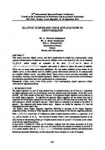
{z } | {z } VE6� VE� Figure 3.1: A diagram of the elliptic quadric from the point of view of the stabilizer of two points.
Figure 3.1 is a diagram of E from the point of view of the stabilizer Gl of {(1, 0, 0, 0), (0, 1, 0, 0)}.
The horizontal lines represent planes in FE,
and the vertical lines represent planes in VE. The planes VE meet in l⊥ = h(0, 0, 1, 1), (0, 0, 1, −1)i and the planes FE meet in l = h(1, 0, 0, 0), (0, 1, 0, 0)i. The points of E\{(1, 0, 0, 0), (0, 1, 0, 0)} are on the lines in orbits L∩E = VE� ∩FE�
31
and L6∩E = VE6� ∩ FE6� under the action of Gl� .
Each dot represents a
line of L∩E containing a pair of points (1, a2 − ηb2 , a, b), (1, a2 − ηb2 , −a, −b), (a, b) 6= (0, 0). The intersections without dots represent the lines in the orbit of m′ = h(1, η, 1, 0), (1, η, −1, 0)i, L6∩E under Gl . Under the action of Gl� , the four quadrants of the grid each represent an orbit of lines. Each of these four orbits of lines carries orbits of planes distinct from FE and VE. In the next chapter, we will study how the planes in an orbit carried by an orbit of lines in a quadrant of the grid meet E� . We will see that it is sufficient to study planes in orbits of ω6∩ the type Oω∩ E� and in orbits of the type OE� .
3.4.3 The Square Points of H Let H� = {(1, s2 − t2 , s, t) : s2 − t2 ∈ �}, the subset of H analogous to E� ⊆ E. That is, H� is the set of points of H corresponding to the set of all (a, b) such that a2 − b2 is a nonzero square. The group Hl� stabilizing H� is generated by {̟a,b : a2 − b2 ∈ �}, M and N and [Hl : Hl� ] = 2. It is straightforward to show that, under the action of Hl� , the points on l are in three orbits: {(1, 0, 0, 0), (0, 1, 0, 0)}, {(1, s2 , 0, 0) : s ∈ F∗q } and {(1, ηs2 , 0, 0) : s ∈ F∗q }. Similarly, there are three orbits of points on l⊥ : {(0, 0, 1, 1), (0, 0, 1, −1)}, {(0, 0, a, b) : a2 –b2 ∈ �} and {(0, 0, a, b) : a2 –b2 ∈ � 6 }. The orbit under Hl , L∩H splits into two orbits under Hl� : L∩H� and L∩H6� , which contain the points of H� and H6� , respectively. Similarly, the orbit of lines L6∩H splits into the two orbits L6∩H� and L6∩H� under the action of Hl� .
32
Theorem 3.4.4 The orbits of planes under the action of Hl� are as follows: 1. The tangent planes [0, 1, 0, 0]T and [1, 0, 0, 0]T to the points (1, 0, 0, 0) and (0, 1, 0, 0), respectively form an orbit of size 2. 2. The tangent planes [0, 0, 1, −1]T and [0, 0, 1, 1]T to the points (0, 0, 1, 1) and (0, 0, 1, −1), respectively form an orbit of size 2. 3. The planes VH� = {πc� } = {[1, −c−1 , 0, 0]T : c ∈ �}, form an orbit of size q − 1. 4. The planes VH6� = {πc6� } = {[1, −c−1 , 0, 0]T : c ∈ � 6 }, form an orbit of size q − 1. 5. The planes FH� = {γa,b = [0, 0, a, b]T } on the line h(1, 0, 0, 0), (0, 1, 0, 0)i such that αa,b ∩ H� = {(1, s2 − t2 , s, t) : s2 − t2 ∈ � and sa + tb = 0} ∪ {(1, 0, 0, 0), (0, 1, 0, 0)} form an orbit of size
q−1 . 2
6. The planes FH� = {γa,b = [0, 0, a, b]T } on the line h(1, 0, 0, 0), (0, 1, 0, 0)i such that αa,b ∩ H = {(1, s2 − t2 , s, t) : s2 − t2 ∈ � and sa + tb = 0} ∪ {(1, 0, 0, 0), (0, 1, 0, 0)} form an orbit of size
q−1 . 2
7. The planes FH6� = {γa,b = [0, 0, a, b]T } on the line h(1, 0, 0, 0), (0, 1, 0, 0)i such that αa,b ∩ H� = {(1, s2 − t2 , s, t) : s2 − t2 ∈ 6� and sa + tb = 0} ∪ {(1, 0, 0, 0), (0, 1, 0, 0)} form an orbit of size
q−1 . 2
8. The planes meeting exactly one of (1, 0, 0, 0) or (0, 1, 0, 0) and one point on h(0, 0, 1, 1), (0, 0, 1, −1)i \ {(0, 0, 1, 1), (0, 0, 1, −1)} ∩ γa,b for some γa,b ∈ FH� form a single orbit of size (q − 1)2 .
33
9. The planes meeting exactly one of (1, 0, 0, 0) or (0, 1, 0, 0) and one point on h(0, 0, 1, 1), (0, 0, 1, −1)i \ {(0, 0, 1, 1), (0, 0, 1, −1)} ∩ γa,b for some γa,b ∈ FH6� form a single orbit of size (q − 1)2 . 10. The planes on exactly one of the lines h(1, 0, 0, 0), (0, 0, 1, 1)i, h(0, 1, 0, 0), (0, 0, 1, 1)i, h(0, 1, 0, 0), (0, 0, 1, −1)i, or h(1, 0, 0, 0), (0, 0, 1, −1)i form an orbit of size 4(q − 1). 11. The
q−1 2
∗ orbits Oω∩ H� , ω ∈ Fq of size
(q−1)2 2
such that [1, −1, 0, ω] ∈ Oω∩ H�
This includes a single orbit O2∩ H� of tangent planes to points of H not on [1, 0, 0, 0]T or [0, 1, 0, 0]T . The tangent planes are the orbit O2∩ H� and are tangent to points of H� when q ≡ 3 mod 4 and are tangent to points of H6� when q ≡ 1 mod 4. 12. The
q−1 2
∗ orbits Oω∩ H6� , ω ∈ Fq of size
(q−1)2 . 2
These are orbits of planes
meeting a single line of L∩H6� . This includes a single orbit of tangent planes to points of H not on [1, 0, 0, 0]T or [0, 1, 0, 0]T . The tangent planes are tangent to points of H� when q ≡ 1 mod 4 and are tangent to points of H6� when q ≡ 1 mod 4. 13. The
q−1 2
∩ orbits Oω6H� , ω ∈ F∗q of size
(q−1)2 2
∩ such that [1, −η −1 , 0, ω] ∈ Oω6H� .
These are orbits of planes containing a single line of L6∩H� . 14. The
q−1 2
orbits Oω6H6∩� , ω ∈ F∗q of size
(q−1)2 . 2
These are orbits of planes
containing a single line of L6∩H6� . Proof: We can check that Hl� is transitive on the four lines in the statement of number 9, via the action of hM, Ni. Consider the action of {̟a,b : a2 − b2 =
34
1} ⊆ Hl� on planes on any of these lines, say β = [0, 1, ω, −ω]T for some ω 6= 0 on h(1, 0, 0, 0), (0, 0, 1, 1)i. β ∩ [0, 0, 0, 1]. If ̟a,b β = ̟c,dβ for some a2 − b2 = c2 − d2 = 1 then we must have a − b = c − d, whence a + b = c + d and hence a = c and b = d. As there are q − 1 representations a2 − b2 of 1, the orbit of β includes all planes on h(1, 0, 0, 0), (0, 0, 1, 1)i which are not tangent to H. Thus the orbit of β has size 4(q − 1). It is straightforward, if occasionally tedious, to verify the remaining statements.
FH : q–1 planes meeting in l
H6�
VH : q–1 planes meeting in l⊥ }| { z
FH6�
H� }
|
FH�
{z } | {z VH6� VH� Figure 3.2: A diagram of the hyperbolic quadric from the point of view of the stabilizer of two points not on any line of the quadric.
The action of the stabilizer of two points of H not on a line of the quadric is similar to the action of Gl on E. Figure 3.2 is a diagram of H from the point of view of the stabilizer Hl of {(1, 0, 0, 0), (0, 1, 0, 0)}. The planes VH meet in l⊥ =
35
h(0, 0, 1, 1), (0, 0, 1, −1)i and the planes FH meet in l = h(1, 0, 0, 0), (0, 1, 0, 0)i. The points of H not contained in either of the planes [1, 0, 0, 0]T or [0, 1, 0, 0]T are on the lines in orbits L∩H = VH� ∩ FH� and L6∩H = VH6� ∩ FH6� under the action of Hl� . Each dot represents a line of L∩H containing a pair of points (1, a2 − b2 , a, b), (1, a2 − b2 , −a, −b), a2 6= b2 . The intersections without dots represent the lines in the orbit of m′ = h(1, η, 1, 0), (1, η, −1, 0)i, L6∩H under Hl . Under the action of Hl� , the four quadrants of the grid each represent an orbit of lines. Each of these four orbits of lines carries orbits of planes distinct from FH and VH. We will see that, for our purposes, it is sufficient to study planes in the
q−3 2
orbits of the type Oω∩ H� and in the
36
q−1 2
∩ orbits of the type Oω6H� .
4. Truncated Quadrics and Elliptic Curves 4.1 Point Counts on Planes Meeting E� In view of Theorem 3.4.2, it is a simple matter to count the points of E� on planes in certain orbits under Gl,�. The planes in FE� each meet E� in q − 1 points and the planes in FE6� do not meet E� . The planes in VE� each meet E� in q + 1 points and the planes in VE6� miss E� . Each plane of OEl� lies on a line n tangent to either (1, 0, 0, 0) or (0, 1, 0, 0) and in a single plane of FE� . Thus the q − 1 planes on n each meet
q−1 2
of the remaining
E� . Similarly, the planes in OEl6� each meet E� in
q+1 2
q 2 −1 2
− (q − 1) points of
points. The tangents to E
meet E� in either 0 or 1 point. Counting the number of points of E� on planes ω6∩ ω6∩ ω∩ in orbits of type Oω∩ E� , OE6� , OE� and OE6� will take considerably more work.
In our discussion of the orbits of planes under the action of Gl , we found that for the
q−1 2
orbits of type Oω∩ E� , the planes on the line m include 2 repre-
sentatives of each of these orbits. Similarly, the planes on the line m′ include 2 representatives of the
q−3 2
∩ . orbits of type Oω6E�
In order to get a feel for the shape of E� , we checked, for small prime values q, the intersection numbers of some planes with E� . Consider the planes on h(1, 1, 1, 0), (1, 1, −1, 0)i distinct from [0, 0, 0, 1]T ∈ F and [1, −1, 0, 0]T ∈ V , i.e., the set P∩E = {αω = [1, −1, 0, ω]T : ω ∈ F∗q }. Note that P∩E contains two representatives, αω and α−ω , from each orbit Oω∩ E� . As an example, in table 4.1 we have the intersection numbers of this family
37
Table 4.1: Intersection numbers of E� with planes in P∩E for q = 263 N
Planes meeting E� in N points
116 118 120 122 124 126 128 130 132 134 136 138 140 142 144 146 148
** ****** ******************** ****** ****************** ****************************** ************ ************************ ************************** ************************ ************ ****************************** ****************** ****** ******************** ****** **
of planes for q = 263. We notice that Table 4.1 is symmetric with respect to q−1 2
= 132, that each plane meets E� in an even number of points and that the
number of points per plane is relatively near 132. For odd primes p < 300, it was observed that these characteristics hold in general. Lemma 4.1.1 Let E� and P∩E be described as above. Then 1 Each plane in P∩E meets E� in an even number of points. 2 For any N, there are an even number of planes of P∩E meeting E� in N points. Proof: Suppose a point of E� is incident with a plane αω = [1, −1, 0, ω]T of P∩E, that is (1, s2 − ηt2 , s, t)[1, −1, 0, ω]T = 1 − s2 + ηt2 + ωt = 0.
38
(4.1)
If s 6= 0 then (1, s2 − ηt2 , −s, t) is also on αω . If s = 0, solve the quadratic in t and note that the discriminant ω 2 − 4η is nonzero and the roots are distinct. Check also that these roots can never be zero. This proves 1. For 2, simply note that (1, s2 − ηt2 , s, t) ∈ αω if and only if (1, s2 − ηt2 , s, −t) ∈ α−ω , and that each αω meets the oval {(1, s2 , s, 0) : s ∈ F} ∪ (0, 1, 0, 0) in the points (1, 1, 1, 0) and (1, 1, −1, 0). The remainder of this chapter will be concerned primarily with the proof of the following statements, and corresponding statements for the families of orbits of ∩ ω6∩ planes Oω6E� , Oω∩ H� , and OH� .
1. If a plane of P∩E meets E� in N points, then 2. If there is a plane of P∩E meeting E� in
q+1 2
q+1 2
−
√
q≤N ≤
q+1 2
+
√
q.
− t points for some integer t,
then there exists a plane of P∩E which meets E� in
q+1 2
+ t points.
We will see that the second statement, and the corresponding statements for planes meeting the hyperbolic quadric H do not hold for all q. Consider the plane αω = [1, −1, 0, ω]T , ω ∈ F∗q secant to E and containing the points (1, 1, 1, 0) and (1, 1, −1, 0). Asking if a point of E� is on αω , there arises the system of equations (1, s2 − ηt2 , s, t)[1, −1, 0, ω]T = 1 − s2 + ηt2 + ωt = 0
(4.2)
s2 − ηt2 − a2 = 0.
(4.3)
We may convert these to the homogeneous polynomials f (x, s, t, a) = x2 − s2 + ηt2 + ωxt
39
(4.4)
g(x, s, t, a) = s2 − ηt2 − a2 .
(4.5)
This allows us to interpret solutions X = (x, s, t, a) to f (X) = g(X) = 0 as points in projective space P G(3, q). Because η is a nonsquare, s2 − ηt2 = 0 has no solution, so f (0, s, t, a) = 0 has no solution and a point P satisfying f (P ) = g(P ) = 0 may be assumed to have the form P = (1, s, t, a). If P = (1, s, t, a) is a solution to this system, then so is (1, s, t, −a), and these two points correspond to the single point (1, s2 − ηt2 , s, t) on E� with s2 − ηt2 = a2 . That is, if there are N points satisfying f (X) = g(X) = 0, there are
N 2
points of E� on the
plane [1, −1, 0, ω]T . Each of f and g is a degenerate quadratic form over Fq in variables x, s, t, a with respective 1 0 ω2 0 −1 0 Mf = ω 2 0 η 0 0 0
matrices Mf and 0 0 0 0 Mg = 0 0 0 0
Mg , 0
0
0
1 0 0 . 0 −η 0 0 0 −1
Let Cf and Cg be the corresponding quadrics in P G(3, q). Then Cf is a quadratic
cone with vertex (0, 0, 0, 1) and a convenient carrier plane is [0, 0, 0, 1]T . The quadric Cg is a quadratic cone with vertex (1, 0, 0, 0) and carrier plane [1, 0, 0, 0]. Note that neither of the vertices is a point on the other cone, so the cones do not share a linear component. With this choice of carrier planes, the vertex of each cone is on the carrier plane of the other. We postpone the continuation of this discussion in order to outline some relevant results from algebraic geometry and the general theory of elliptic curves.
4.2 Some Background on Elliptic Curves
40
This section collects basic results from algebraic geometry from [21] and [15] and on elliptic curves in particular from [22], [16], and [25] which is necessary to justify the manipulations in coming sections. The first chapter of Shafarevich [21] is particularly illuminating. Let f1 and f2 be homogeneous polynomials over an algebraically closed field K and let C1 and C2 be projective plane curves defined by Ci = {x ∈ P G(2, q) : fi (x) = 0} for i = 1, 2. A rational map from C1 to C2 is a collection of rational functions φ1 , φ2 , φ3 such that for x ∈ C1 , Φ(x) = (φ1 (x1 ), φ(x2 ), φ(x3 )) ∈ C2 . The map Φ is a birational equivalence if the functions φj are invertible, that is, if there exist functions ψj , j = 1, 2, 3 such that φj ◦ ψj and ψj ◦ φj are the identity on the points where the maps are defined. The following theorem is central to our investigations. A proof and discussion may be found in Hartshorne [15], chapter 6. Theorem 4.2.1 Every curve is birationally equivalent to a nonsingular projective curve which is unique up to isomorphism. The genus of an algebraic curve is a nonnegative integer associated with the curve which is invariant under birational transformation. Conics, for example, are curves of genus g = 0. For curves over arbitrary fields, genus may be defined algebraically via the Riemann-Roch theorem. We again refer to Chapter 2 of [22]. An elliptic curve is an algebraic curve of genus 1. It can be shown (Silverman [22], Chapter 2) that any elliptic curve is isomorphic to an affine curve E, together with a point (∞) whose points (x, y)
41
satisfy an equation y 2 + a1 xy + a3 y = x3 + a2 x2 + a4 x + a6 ,
(4.6)
an equation in Weierstrass form, with coefficients in a field K. Any such curve is isomorphic to a curve in the projective plane with an equation y 2z + a1 xyz + a3 yz 2 = x3 + a2 x2 z + a4 xz 2 + a6 z 3 via the map (x, y) → [1, x, y], (∞) → [0, 1, 0] and conversely that any nonsingular curve given by a Weierstrass equation is an elliptic curve. Any isomorphism between curves with equations of the form 4.6 is given by a change of variables x = t2 x′ + u
(4.7)
y = t3 y ′ + vx′ + s
(4.8)
with s, t, u, v ∈ K and t 6= 0, where K is the algebraic closure of K. See [16], Chapter 3 for proof. We call this an admissible change of variables. If the characteristic of K is not 2 or 3, equation 4.6 can always be transformed to an equation of the form y 2 = x3 + Ax2 + Bx + C
(4.9)
via an admissible change of variables. An elliptic curve is necessarily nonsingular, that is, it has no points (x, y) at which both partial derivatives vanish.
42
For a curve with equation y 2 = f (x) as in equation 4.9, this is equivalent to f (x) having distinct roots. We define an elliptic curve to be a nonsingular affine curve whose points satisfy an equation of the form 4.9 together with a point ∞. We now state the Hasse-Weil Theorem, which is essential to our progress. For a curve E, let #E(Fq ) denote the number of Fq -rational points of E. Theorem 4.2.2 (Hasse-Weil) Let E be a projective curve of genus g defined over a finite field Fq . Then √ √ q + 1 − 2g q ≤ N ≤ q + 1 + 2g q.
(4.10)
We refer to [16] or [22] for a proof when g = 1 and [15] for the more difficult result when g is arbitrary. 4.3 Birational Transformations Between Quartics and Cubics In this section, we carry out algebraic transformations on equations of curves whose points correspond to the points on the intersections of planes with the truncated quadrics. The resulting equations are of the form 4.9, and we apply the Hasse-Weil Theorem with g = 1. 4.3.1 Elliptic Curves From Orbits O∩E� We return to the equations 4.4 and 4.5 from section 4.1. These equations arose from considering the intersection of a plane πω = [1, −1, 0, ω]T with E. From g(x, s, t, a) = 0 we have s2 − ηt2 = a2 , which we substitute into equation 4.4 to get x2 − a2 + ωt = 0 . We may assume that x 6= 0, since no point on Cf ∩ Cg is of the form (0, s, t, a). We solve for t t=
a2 − x2 ωx
43
and substitute into g(x, s, t, a) = 0 to obtain, after simplification F (x, s, a) = ηx2 + (ω 2 − 2η)x2 a2 + ηa2 − ωx2 s2
(4.11)
and we let CF = {(x, s, a) ∈ P G(2, q)|F (x, s, a) = 0} be the corresponding plane curve. When x = 0, there is the unique solution (0, 1, 0). Put x = 1 in F (x, s, a) = 0 to obtain the equation ω 2 s2 = ηa4 + (ω 2 − 2η)a2 + η,
(4.12)
the affine part of CF . We will show that equation 4.12 is birationally equivalent to an equation for an elliptic curve in Weierstrass form, that is, an equation of the form 4.9. Our hypothesis that Fq is an arbitrary finite field of odd order does not change. In particular, these manipulations are justified when Fq has characteristic 3. Our method follows one outlined in chapter 8 of Cassels [8]. Note that the point (a, s) = (1, 1) satisfies equation 4.12. Put1 u =
1 , a−1
to obtain (after
dividing through by ω 2) s2 =
η 1 (ω 2 − 2η) 1 η 4 ( + 1) + ( + 1)2 + 2 2 2 ω u ω u ω
which leads to u4 s2 = u4 + 2u3 +
η ω 2 − 2η 2 4η u + 2u + 2. 2 ω ω ω
Put v = su2 and write the right hand side as G(u)2 + H(u), where G(u) = u2 + g1 u + g0 and 1
The first step has the effect of moving the rational point (1, 1) to ∞ on the resulting elliptic curve and is not absolutely essential.
44
H(u) = h1 u + h0 . solving for coefficients we find g1 = 1, g0 =
2η , ω2
h1 = 0 and h0 =
η ω2
−
4η2 . ω4
Now
v 2 = G(u)2 + H(u), so (v + G(u))(v − G(u)) = H(u). Put v + G(u) = t, whence v − G(u) =
H(u) H(u) and then 2G(u) = t − . t t
Multiply through by 4t2 to obtain � � η 4η 2 2η 2 3 − 4 t. 4u t + 4ut + 2 t = 2t − 2 ω ω2 ω 2 2
2
Let d = ut, so that 2η 4d + 4dt + 2 t2 = 2t3 − 2 ω 2
and then let r = 2d + t, so that d =
r−t 2
3
η 4η 2 − ω2 ω4
�
t
and after simplification
�
η� r = 2t + 1 − 8 2 t2 − 2 ω 2
�
�
η η2 − 4 ω2 ω4
�
t.
Finally put y = 2r and x = 2t to put our equation into a rather nice form: � � � 16η 2 4η η � 2 − 2 x y =x + 1−8 2 x + ω ω4 ω � �� � 2 4η 4η − ω y2 = x x − 2 x− ω ω2 2
3
(4.13)
ω and let EE� , together with ∞, be the elliptic curve whose points satisfy this
equation. Tracing through the various transformations, we find that the rational maps a=
2x +1 y−x
45
(4.14)
2x3 + (1 − 8 ωη2 )x2 − y 2 s= (y − x)2
(4.15)
4ηa2 + 2(ω 2 − 4η)a + 4η + 2ω 2s ω 2(a − 1)2
(4.16)
4ηa3 + 2(ω 2 − 2η)a2 + 2(ω 2 (s + 1) − 2η)a + 2(2η + ω 2 s) (a − 1)3 ω 2
(4.17)
with inverse maps x= y=
ω map the curve with equation 4.12 to the affine part of E = EE� . The functions
from E to CF are undefined only when a = 1, and the inverse functions are undefined only when x = y. If we put y = x in equation 4.13, we find that for x 6= 0, the discriminant of the resulting quadratic is
16η , ω2
which is never a square
in Fq . Thus the only point on 4.13 with x = y is (0, 0) and so the only rational points of E on which the maps 4.16 and 4.17 are undefined are (0, 0) and ∞. The two points of CF for which a = 1 are (1, 1) and (1, −1). We extend the rational maps between CF and E by (1, 1) ↔ ∞ and (1, −1) ↔ (0, 0). Thus augmented, the rational maps 4.14 and 4.15 and their inverses 4.16 and 4.17 give a bijection between the points of E (including ∞) and the nonsingular points of the projective curve CF that is, the points of CF different from (0, 1, 0). Two nonsingular points (s, a), (s, −a) on CF correspond to the single point (1, s2 − ηt2 , s, t) with s2 − ηt2 = a2 on αω ∩ E� , where t =
a2 −1 . ω
Thus the map
from the points of the elliptic curve E to the points on αω ∩ E� is 2:1, and by the Hasse-Weil Theorem we have the following result. Theorem 4.3.2 Let αω , ω ∈ F∗q be a plane in the orbit Oω∩ E� and let Nω = |αω ∩ E� |. Then Nω is even and q+1 √ q+1 √ − q ≤ Nω ≤ + q. 2 2
46
(4.18)
ω∩ ω∩ Let EE� denote the elliptic curve with equation 4.13 and E∩E� = {EE� }ω∈F∗q . √ In our example q = 263 in Figure 4.1, we find ⌊264+2 263⌋ = 296 = 2(148)
which shows that the bounds of 4.18 are as close as possible without some further restriction. 4.3.3 Elliptic Curves From Orbits O6∩E� Let P6∩E = {[1, −η −1, 0, ω]T : ω ∈ Fq \ {0, 2, −2}}. We choose a representa∩ tive plane αω = [1, −η, 0, ω]T in the orbit Oω6E� . Note that [1, −η −1 , 0, ±2]T are
tangent planes to E at the points (1, −η, 0, ±1), hence the restriction. From the equations (1, s2 − ηt2 , s, t)[1, −η, 0, ω]T = 1 − η(s2 − ηt2 ) + ωt = 0 s2 − ηt2 − a2 = 0 we obtain the equation ηω 2 s2 = a4 + η(ω − 2)a2 + η 2 .
(4.19)
The substitution √
ηx y √ η(4x3 + x2 (2 − ω 2 ) − 2y 2 s= 2ωy 2
a=
(4.20) (4.21)
transforms 4.19 to � � 4 2 − ω2 2 ω ω2 y =x + x x + − 2 16 4 �� � 2 �� � ω ω2 x− −1 =x x− 4 4 2
3
47
(4.22)
which is nonsingular whenever ω 6= ±2. The inverse rational maps are −2a2 + 2η + 2ηωs + ω 2 a2 and 4a2 3 √ √ −2a2 η + η 2 + 2ηωs + ηω 2 a2 y= . 4a3
x=
(4.23) (4.24)
Again we apply the Hasse-Weil theorem and find that for Nω = |αω ∩ E� |, ω 6= ±2 q+1 √ q+1 √ − q ≤ Nω ≤ + q. 2 2
(4.25)
When ω = ±2, the equation 4.22 is singular and the curves correspond to the planes tangent at the points (1, −η, 0, ±1). When q ≡ 3 mod 4, −η is a square and the points (1, −η, 0, ±1) are on E� , while when q ≡ 1 mod 4 they are on E6� . The total number of points of E� on the planes αω , ω ∈ Fq \ {0, 2, −2} is therefore
(q−1)2 2
when q ≡ 1 mod 4 and
q 2 −2q−3 2
when q ≡ 3 mod 4.
4.3.4 Elliptic Curves from Orbits O∩H� Now consider H� , a subset of the hyperbolic quadric H defined in Section 3.5 and stabilized by the group Hl� . We look first at planes in the orbits O∩H. Similar to the situation with planes in orbits O6∩E� when ω = ±2, the planes are tangent to H at the points (1, −1, 0, ±1). These points are on H� when q ≡ 3 mod 4 and on H6� when q ≡ 1 mod 4. From the system of equations (1, s2 − t2 , s, t)[1, −1, 0, ω]T = 1 − s2 + t2 + ωt = 0 2
2
(4.26)
2
s −t −a =0 we obtain the quartic ω 2 s2 = a4 + (ω 2 − 2)a2 + 1
48
(4.27)
which is equal to 4.19 if we set η = 1 in that equation. We adapt the birational maps from the discussion of planes in O∩E. The rational maps x y (4x3 + x2 (2 − ω 2 ) − 2y 2 s= 2ωy 2
a=
(4.28)
take 4.27 to � � 4 ω ω2 2 − ω2 2 x x + − y =x + 2 16 4 �� � 2 � �� ω ω2 x− =x x− −1 4 4 2
3
(4.29) (4.30)
which is identical to equation 4.22. The inverse maps are −2a2 + 2 + 2ωs + ω 2 a2 4a2 2 −2a + 1 + 2ωs + ω 2 a2 . y= 4a3
x=
(4.31) (4.32)
Although the curves that arise here are isomorphic to those from orbits Oω∩ E� , the point counts on planes are slightly different. Note that the plane [1, −1, 0, ω]T meets H in the four points (1, 0, ±ω −1, −ω −1 ) and (0, 1, ±ω −1, ω −1 ) which are not in H� . These pairs of points lie on the planes [0, 1, 0, 0]T and [1, 0, 0, 0]T tangent to H at (1, 0, 0, 0) and (0, 1, 0, 0), respectively. Let βω be a plane in the orbit Oω∩ H� , and Nω = |βω ∩ H� |. Then q−3 √ q−3 √ − q ≤ Nω ≤ + q 2 2 by the Hasse-Weil Theorem. 4.3.5 Elliptic Curves from Orbits O6∩H�
49
(4.33)
∩ , which contains the planes [1, −η, 0, ±ω]T on the line Consider an orbit Oω6H�
h(1, η −1, 1, 0), (1, η −1, −1, 0)i. Note that for all ω ∈ F∗q , these planes are secant to H. From the system (1, s2 − t2 , s, t)[1, −η, 0, ω]T = 1 − η(s2 − t2 ) + ωt = 0 2
2
(4.34)
2
s −t −a =0 we obtain the quartic �
ωs η
�2
= a4 +
ω 2 − 2η 2 1 a + 2 2 η η
(4.35)
which we transform to the cubic 2η − ω 2 2 ω 4 − 4ηω 2 x + x y 2 = x3 + 2η 2 16η 4 � �� � ω2 ω 2 − 4η =x x− 2 x− 4η 4η 2
(4.36)
ω6∩ using the technique from Section 4.3.1. Let EH� be the curve with equation ω6∩ 4.36 and E6∩H� = {EH� : ω ∈ F∗q }. The plane αω = [1, −η, 0, ω]T meets the
plane [0, 1, 0, 0]T at the points (1, 0, ±ω −1, −ω −1 ) and (0, 1, −ω −1, −ω −1 ) of H, which are not points of H� . The points (1, 0, ±ω −1, −ω −1) give two solutions (s, t, a) = (−ω −1 , ±ω −1 , 0) to the system 4.34. Thus the number of solutions (s, t, a) to 4.34 is two more than |αω ∩ H� |. ∩ To reiterate, let αω be a plane in the orbit Oω6H� , and Nω = |αω ∩ H� |. Then
by the Hasse-Weil Theorem, q−3 √ q−3 √ − q ≤ Nω ≤ + q. 2 2
4.3.6 Families of Curves
50
(4.37)
2
Return now to equation 4.36 and make the substitution x 7→ x + ω 4η−4η 2 . �6 and make the substitutions y 7→ Multiply both sides of the result by 2η ω � �3 � �2 ω ω y and x 7→ 2η x, to obtain 2η �
4η y =x x− 2 ω 2
�� � 4η − ω 2 x− ω2
(4.38)
which is identical to equation 4.13. That is, the families of curves E∩E� and E6∩H� are the same. To reiterate the relationship between curves from H� and from E� , we state the following theorem. Theorem 4.3.7 The set of elliptic curves E∩E that arise from considering the intersections of planes in P∩E with E� is identical with the set of elliptic curves E6∩H which arise from considering the intersections of planes in P6∩H with H� . The set of elliptic curves E6∩E that arise from considering the intersections of planes in P6∩E with E� is identical with the set of elliptic curves E∩H which arise from considering the intersections of planes in P∩H with H� . Thus we have two families of elliptic curves to consider, and they take surprisingly simple forms. Make the substitution a =
2 ω
into equation 4.13, and
write E∩E = {y 2 = x x − ηa2
�
x − ηa2 − 1
��
: a ∈ F∗q }.
(4.39)
From equation 4.22, we obtain, via the substitution a = ω2 , the set of curves E6∩E = {y 2 = x x − a2
�
x − a2 − 1
51
��
: a ∈ Fq \ {0, 1, −1}}.
(4.40)
4.4 Summary of Plane Intersections with Truncated Quadrics In this section, we give a complete summary of plane intersections with E� and H� in terms of exact counts or bounds given by the Hasse-Weil Theorem. We first explain how the bounds we have found give bounds on orbits we have not yet considered. 4.4.1 Other Plane Orbit Types ω6∩ ω6∩ ω∩ We turn now to the orbits of planes Oω∩ E6� , OE6� , OH6� , and OH6� and their
intersections with E� and H� . These orbits have the same relationship with E6� and H6� as the orbits we have already considered have with E� and H� , and the point counts of the intersections are easily calculated. Choose a, b ∈ Fq such that a2 − ηb2 = η. Then ϕa,b ∈ Gl interchanges E� with E6� and in particular, (1, 1, 1, 0)ϕa,b = (1, η, a, b) and (1, 1, −1, 0)ϕa,b = (1, η, −a, −b), so the set PE� is exchanged with a set of representatives for orbits Oω∩ E6� . As each non-tangent plane of P G(3, q) meets E in q + 1 points, the number N6�ω of points of E� on the plane [1, −η −1 , −ωbη −1 , ωaη −1]T ∈ Oω∩ E6� is equal to the number of points of E6� on [1, −1, 0, ω]T . By our application of the Hasse-Weil Theorem to the number of points on planes in Oω∩ E� , we have q+1 √ q+1 √ − q ≤ NE6ω� ≤ + q. 2 2 We obtain the same bounds on the number of points of E� on planes in orbits ∩ ∩ by counting the number of points of E6� on planes in orbits Oω6E� of type Oω6E6� ∩ ∩ with ϕa,b , which simultaneously interchanges E� and to Oω6E6� and mapping Oω6E�
52
E6� . Thus if a plane π of P G(3, q) meets E in q + 1 points of which
q+1 2
+ t are
points of E� , then an element of Gl taking E� to E6� (such as ϕa,b as defined previously) takes π to a plane ϕa,b π meeting E6� in E� in
q+1 2
q+1 2
+ t points, so ϕa,b π meets
− t points. We call this a complementarity property.
Similarly, if we choose c and d ∈ Fq such that c2 − d2 = η, then ̟c,d ∈ Hl interchanges the points of H� with the points of H6�, and takes orbits Oω∩ H� and ∩ ω6∩ to orbits Oω∩ Oω6H� H6� and OH6� , respectively. We may choose as a representative
plane in an orbit of type O∩H� the plane πω = [1, −1, 0, ω] for some ω 6= 0. Then πω contains the points (1, 0, ω −1, ±ω −1 ) and (0, 1, ±ω −1, ω −1) of H and so meets H� ∪ H6� in q − 3 points. Thus a complementarity property holds for H as well.
4.4.2 Summary of Plane Intersections for Truncated Quadrics We summarize our results on the plane intersection numbers for E� and for H� in two theorems. Theorem 4.4.3 Let E� = {(1, s2 − ηt2 , s, t) : s2 − ηt2 ∈ �} and let the orbits of planes under Gl� be as stated in Theorem 3.4.2. 1. The
q 2 −1 2
tangent planes to E� each meet E� in a single point.
2. The
q 2 +3 2
tangent planes to E \ E� do not meet E� .
3. The
q−1 2
planes VE6� do not meet E� .
4. The
q−1 2
planes VE� each meet E� in q + 1 points.
5. The planes in FE� each meet E� in q − 1 points.
53
6. The planes in FE6� do not meet E� . 7. The planes in OEl� each meet E� in
q−1 2
points.
8. The planes in OEl6� each meet E� in
q+1 2
points.
∗ 9. Each plane in an orbit Oω∩ E� , ω ∈ Fq each meets E� in N points, where N √ − N| ≤ q. is even and satisfies | q+1 2 ∗ 10. Each plane in an orbit Oω∩ E6� , ω ∈ Fq meets E� in N points, where N is √ even and satisfies | q+1 − N| ≤ q. 2 ∩ 11. Each plane in an orbit Oω6E� , ω ∈ F∗q meets E� in N points, where N is √ − N| ≤ q. even and satisfies | q+1 2 ∩ , ω ∈ F∗q meets E� in N points, where N is 12. Each plane in an orbit Oω6E6� √ − N| ≤ q. even and satisfies | q+1 2
Proof:
When we are able to give an exact value, the number is at most a
consequence of the orbit-stabilizer theorem. The bounds given in statements 9 and 10 are consequences of our application of the Hasse-Weil Theorem, and the bounds in statements 11 and 12 are arrived at via the complementarity property discussed prior to the theorem statement. The structure of H� is slightly more complicated than that of E� , and there are several more orbit types. Theorem 4.4.4 Let H = {1, s2 − t2 , s, t) : s2 − t2 ∈ �} and let the orbits of planes under Hl� be as stated in Theorem 3.4.4. 1. The
(q−1)2 2
tangent planes to H� each meet H� in q − 1 points.
54
2. The
(q−1)2 2
tangent planes to H6� each meet H� in q − 2 points.
3. The planes VH� each meet H� in q − 1 points. 4. The planes VH6� do not meet H� . 5. The planes FH� each meet H� in q − 1 points. 6. The planes FH6� do not meet H� . 7. The planes meeting exactly one of (1, 0, 0, 0) or (0, 1, 0, 0) and one point x on h(0, 0, 1, 1), (0, 0, 1, −1)i \ {(0, 0, 1, 1), (0, 0, 1, −1)} such that x is on a plane of FH� each meet H� in
q−3 2
points.
8. The planes meeting exactly one of (1, 0, 0, 0) or (0, 1, 0, 0) and one point x on h(0, 0, 1, 1), (0, 0, 1, −1)i \ {(0, 0, 1, 1), (0, 0, 1, −1)} such that x is on a plane of FH6� each meet H� in
q−1 2
points.
9. The planes on exactly one of the lines h(1, 0, 0, 0), (0, 0, 1, 1)i, h(0, 1, 0, 0), (0, 0, 1, 1)i, h(0, 1, 0, 0), (0, 0, 1, −1)i, or h(1, 0, 0, 0), (0, 0, 1, −1)i each meet H� in
q−1 2
points.
∗ 10. Planes in an orbit Oω∩ H� , ω ∈ Fq \ {2, −2} each meet H� in N points for √ − N| ≤ q. some N satisfying | q−3 2 ∗ 11. Planes in an orbit Oω∩ H6� , ω ∈ Fq each meet H� in N points for some N √ − N| ≤ q. satisfying | q−3 2 ∩ 12. Planes in an orbit Oω6H� , ω ∈ F∗q each meet H� in N points for some N √ − N| ≤ q. satisfying | q−3 2
55
13. Planes in an orbit Oω6H6∩� , ω ∈ F∗q each meet H� in N points for some N √ − N| ≤ q. satisfying | q−3 2 T 14. Planes in the orbit O2∩ H� of tangent planes to points of H not on [1, 0, 0, 0]
or [0, 1, 0, 0]T each meet H� in q points when q ≡ 1 mod 4 and in q − 1 points when q ≡ 3 mod 4. T 15. Planes in the orbit O2∩ H6� of tangent planes to points of H not on [1, 0, 0, 0]
or [0, 1, 0, 0]T each meet H� in q − 1 points when q ≡ 1 mod 4 and in q points when q ≡ 3 mod 4. Proof: Because Hl� is transitive on the points of H� , and hence on the tangent planes to H� , it is sufficient for 1 to consider the tangent plane [1, 1, −2, 0]T to the point (1, 1, 1, 0). This plane contains 2q + 1 points of H, including (1, 1, 1, 0) and the four points (1, 0, 2−1, ±2−1 ) and (0, 1, 2−1, ±2−1 ). Any element ̟a,b of Hl such that a2 − b2 ∈ � 6 interchanges H� and H6� , and so the points of H� distinct from (1, 1, 1, 0) on [1, 1, −2, 0]T are equal in number to the points of H6� on [1, 1, −2, 0]T . The reasoning for 2 is similar. The other exact counts are either immediate or are a consequence of the orbit-stabilizer theorem. The planes in orbits of type O∩H� and O6∩H� were handled in Sections 4.3 and 4.4. The bounds given in statements 11 and 13 follow by our application of the Hasse-Weil Theorem and the complementarity property.
4.5 Sums of Point Counts In this section, we use our knowledge of the number of incidences of sets of representatives of plane orbits with the truncated quadrics to find the total
56
number of points in the elliptic curve families given in equations 4.39 and 4.40. The planes P∩E = {αω } = {[1, −1, 0, ω]T : ω ∈ F∗q } all meet in the line h(1, 1, 1, 0), (1, 1, −1, 0)i and partition the points of E� which do not lie on either [0, 0, 0, 1]T or [1, −1, 0, 0]T . Thus the number of incidences of {αω } ∩ E� is seen to be
q 2 −1 . 2
As the map taking points of E� ∩ αω to points
on the associated elliptic curve is 1 : 2, the total number of points on the family ω∩ of curves E = {EE� } is q 2 − 1, including multiplicities.
Now we have the problem of finding how the points of H� are partitioned ω6∩ by the set of planes on a single line in an orbit Lω∩ H� or LH� . On the line
h(1, 1, 1, 0), (1, 1, −1, 0)i ∈ LH� , each pair of planes [1, −1, 0, ±ω], ω ∈ F∗q are T in a distinct orbit Oω� H� . We will write αω = [1, −1, 0, ω] . When ω = ±2, the
planes αω are the tangents to H at the points (1, −1, 0, 1) and (1, −1, 0, −1). In [1, −1, 0, −2]T , the plane tangent at (1, −1, 0, 1), the tangent lines to H may be written n1 = {(1, 1 + 2λ, 1 + λ, −λ) : λ ∈ Fq } ∪ {(0, 2, 1, −1)} and n−1 = {(1, 1 + 2λ, −1 − λ, −λ) : λ ∈ Fq } ∪ {(0, 2, −1, −1)}. The points (0, 2, ±1, −1) are on the plane [1, 0, 0, 0]T tangent at (0, 1, 0, 0). The points (1, 1 + 2λ, 1 + λ, λ) and (1, 1 + 2λ, −1 − λ, −λ) are the unique points of n1 and n−1 on the plane [1, −(1 + 2λ)−1 , 0, 0] ∈ VH. Thus [1, −1, 0, −2]T meets H� in q points when −1 is a square in Fq and in q − 1 points when −1 is a nonsquare. In this way we find the same counts for points of H� on the plane [1, −1, 0, 2]T .
2
Let N be the set
of points of H� on one of the planes [0, 0, 0, 1]T , [1, −1, 0, 2]T or [1, −1, 0, −2]T . The planes in the set P∩H = {αω = [1, −1, 0, ω]T : ω 6= 0, 2, −2} each contain 2
It is possible that we could have made a more geometric argument here.
57
(1, 1, 1, 0) and (1, 1, −1, 0) and each of the
q 2 −4q+6−4d 2
points of H� \ N are on
exactly one of these planes, where d = q − 1 when q ≡ 3 mod 4 and d = q when q ≡ 1 mod 4. Each plane in P∩H contains (1, 1, 1, 0) and (1, 1, −1, 0) and meets 2 points of H ∩ [1, 0, 0, 0]T . In particular, αω = [1, −1, 0, ω] contains the points (0, 1, ω −1, ω −1) and (0, 1, −ω −1, ω −1 ). Thus the planes of P∩H have a total of
q 2 −6q+9 2
incidences with points of H� ∩ ([1, 0, 0, 0]T ∪ H), counting the 2(q − 3)
incidences from {αω } meeting (1, 1, 1, 0) and (1, 1, −1, 0). Each such incidence yields 2 points on the curve with equation 4.29. Each curve also has 4 points corresponding to the 2 points on the intersection αω ∩ H ∩ [0, 1, 0, 0]T . This proves the following theorem. Theorem 4.5.1 The family of elliptic curves E∩E
η = {y = x + (1 − 8 2 )x2 + ω 2
3
�
16η 2 4η − 2 ω4 ω
�
x : ω ∈ F∗q }
contains a total of q 2 − 1 Fq -rational points. The family of elliptic curves E6∩E = {y 2 = x3 +
ω4 ω4 2 − ω2 2 x + ( − )x : ω ∈ Fq \ {0, 2, −2}} 2 16 4
contains a total of q 2 − 2q − 3 Fq -rational points. 4.6 The Invariant j and Symmetry of Incidences In this section, we show that for the family of planes P∩E = {αω } = {[1, −1, 0, ω]T }, ω ∈ F∗q , the planes meeting E� in
q+1 2
+ t points are in one-
to-one correspondence with the planes in P∩E meeting E� in
q+1 2
− t points. To
prove this result, we require more elementary properties of elliptic curves. Proofs and further discussion of these results may be found in [16] and [22]. For our
58
results in Section 4.6.2 and beyond, we find it necessary to restrict ourselves to finite fields Fq where q = pe and p > 3. 4.6.1 Admissible Changes of Variables For the finite field Fq , let Fq denote the algebraic closure of Fq . As usual, ω ∈ F∗q and η is a nonsquare in Fq . Two elliptic curves with Weierstrass equations y12 = f (x1 ) and y22 = g(x2 ) with coefficients in Fq are isomorphic over Fq if and only if there exists a linear change of variables of the form x1 = u2 x2 + r 3
(4.41)
2
y1 = u y2 + su x2 + t ∗
where r, s, t ∈ Fq and u ∈ Fq . The curves E = {(x, y) : y 2 = x3 + ax2 + bx + c} ∪ {(∞)} and E η = {(x, y) : ηy 2 = x3 + ax2 + bx + c} ∪ {(∞)} are seen to be isomorphic over Fq , via the substitution y 7→
√
η −1 y. In this case
we say that E η is a twist of E by η. E and E η are isomorphic over Fq2 , and since any nonsquare β ∈ Fq may be written β = ηα2 for some α ∈ Fq , the twist of E is unique up to isomorphism. Proposition 4.6.2 Let E and E η be elliptic curves given by y 2 = f (x) and ηy 2 = f (x), respectively, where f (x) = x3 + ax2 + bx + c and let #E be the number of points on E over Fq . Then #E + #E η = 2(q + 1). Proof: For each zero x of f , the point (x, 0) is on both E and E η . Say f has m zeros. Then for each of the remaining q − m elements x of Fq , f (x) is either
59
square or nonsquare, yielding two points on either E or E η . The two points at infinity give the desired sum. Recall that the curve Eω from the plane πω in orbit Oω∩ E� has k points if and k 2
only if the plane αω meets E� in exactly
points. To show that the symmetry
of incidences observed in Section 4.1 holds for all q, by Proposition 4.6.2 it will be sufficient to show that for ω 6= 0, the elliptic curve Eω = {(x, y) : y 2 = 2
x3 + (1 − 8 ωη2 )x2 + ( 16η − ω4
4η )x} ω2
∪ {(∞)} has as a twist the curve Eδ for some
−1
δ 6= 0. Consider the twist Eωη
� � � η� 2 16η 2 4η η y =x + 1−8 2 x + − 2 x ω ω4 ω −1 2
3
and make the substitutions x 7→ a−2 η −1 x + r and y 7→ a−3 η −1 y, yielding a2 η(ω 2(3r + 1) − 8η) 2 x + ω2 a4 η 2 (16η 2 − 4ηω 2(4r + 1) + rω 4(3r + 2) x+ ω4 a6 η 3 r(16η 2 − 4ηω 2(2r + 1) + rω 4 (r + 1)) ω4
y 2 = x3 +
after clearing denominators. Put r =
4η−ω 2 ω2
and a =
ω 2η
to obtain, after simplifi-
cation y 2 = x3 +
2η − ω 2 2 ω 4 − 4ηω 2 x + x. 2η 16η 2
Multiply the numerator and denominator of the coefficient on x2 by
� 4η 2 1 , ω 2η
and multiply the numerator and denominator of the coefficient on x by whence 2
3
y =x +
1−8
η � 4η 2 ω
!
2
x +
60
4η 16η 2 � − 4η �2 4η 4 ω
ω
!
x.
� 4η 2 , 2 ω
So the curve Eδ is a twist of Eω when δ =
4η . ω
Note that
4η ω
= ω implies η =
� ω 2 , 2
contrary to the assumption that η is a nonsquare, so δ 6= ω. Thus for each Eω
in E∩E with q + 1 + t points, there is a different curve Eδ in E∩E with q + 1 − t points. This proves the following theorem. Theorem 4.6.3 In the family of elliptic curves over Fq � � � � � 16η 2 4η η � 2 ∗ ∩ 2 3 − 2 x : ω ∈ Fq , EE = y = x + 1 − 8 2 x + ω ω4 ω
if Eω is a curve in E∩E then Eωη is in E∩E as well. Further, if a particular curve
Eω is represented k times in E∩E then Eωη is represented k times in E∩E. We can restate this in terms of the plane intersections αω ∩E� . If αω meets E� in q+1 + 2t 2
points, then αδ meets E� in
q+1 − 2t 2
points, where δ =
4η . ω
The statement
of the relevant theorem for plane intersections is part of Theorem 4.6.6. We might ask how often these complementary pairs of planes (and complementary pairs of elliptic curves) occur in our various families. To find an answer to this, we invoke more of the theory of elliptic curves. For the remainder of this section, assume that we are working over a finite field Fq , where q = pe f or some positive integer e and for a prime p > 3. 4.6.4 The Invariant j To an elliptic curve given by a Weierstrass equation with coefficients in a field F, it is possible to associate a value j ∈ F, the j-invariant of the curve that is invariant under an admissible change of variables, 4.41. Thus any two curves with the same j-invariant are isomorphic over the algebraic closure of F. For curves with Weierstrass equation y 2 = x3 + ax2 + bx, the j-invariant is given by j=
256(a2 − 3b)3 . b2 (a2 − 4b)
61
(4.42)
For details of the derivation and properties of j, see Chapter 3, section 3 of [16]. The curves given by equation 4.13 for ω ∈ F∗q are the curves E∩E and were shown to be isomorphic, as a set, to the curves E6∩H. Further, we found that whenever a curve Eω is in the set E∩E
η � = {y = x + 1 − 8 2 x2 + ω 2
3
�
�
16η 2 4η − 2 ω4 ω
�
x : ω ∈ F∗q }
(4.43)
a quadratic twist Eωη of that curve is also in E∩E, and that a curve and its twist occur the same number of times. From formula 4.42, the j invariants for this family of curves are j=
16(16η 2 − 4ηω 2 + ω 4 ) η 2 ω 4 (4η − ω 2 )2
(4.44)
for ω ∈ F∗q . We have already seen that the curves Eω and E 4η are proper twists ω
of one another, (and so are isomorphic over Fq2 but not necessarily isomorphic over Fq ) and that Eω and E−ω are isomorphic over Fq . Solving 16(16η 2 − 4ηδ 2 + δ 4 ) 16(16η 2 − 4ηω 2 + ω 4 ) = η 2 δ 4 (4η − δ 2 )2 η 2 ω 4 (4η − ω 2 )2
(4.45)
for δ, the solution set is ( ) p √ 2 − 4η 2 p ηω 2 4η ηω 2 4η ±ω, ± , ± p , ± 4η − ω 2 , ± p , ± 2 ω ω 4η − ω ω 2 − 4η
and we find that there are at most 12 values of δ such that Eω ∼ = Eδ over Fq . For the curves E6∩E
2 − ω2 2 x + = {y = x + 2 2
3
�
ω4 ω2 − 16 4
�
x : ω ∈ F∗q , ω 6= ±2}
the j-invariants are j=
16(ω 4 − 4ω 2 + 16)3 ω 4 (ω 2 − 4)2
62
ω ∈ F∗q \ {2, −2}
and in this case the values of δ such that Eω ∼ = Eδ are √ � √ 2 4 4 ω2 − 4 2ω 2 , ± 4 − ω , ±√ ,± δ ∈ ±ω, ± , ± √ . (4.46) ω ω 4 − ω2 ω2 − 4 �
The curves Eω and E 4 are easily seen to be isomorphic over Fq . When q ≡ ω
2
1 mod 4, ω − 4 and 4 − ω 2 are either both square or both nonsquare. A simple count shows that for some values of ω, both ω 2 − 4 and 4 − ω 2 are nonsquare. Thus it is possible that the family of curves E6∩E does not contain a proper twist of Eω for every ω ∈ F∗q . When q ≡ 3 mod 4, exactly one of ω 2 − 4 or 4 − ω is a square, and it is straightforward to check that for each ω ∈ Fq , at least one value of δ in 4.46 gives a twist of Eω by −1. We interpret this result in terms of plane intersections with E� and H� . Theorem 4.6.5 Assume that q ≡ 3 mod 4. Let P∩H = P∩E = {[1, −1, 0, ω] : ω ∈ F∗q , ω 6= ±2} and P6∩H = P6∩E = {[1, −η −1 , 0, ω] : ω ∈ F∗q , ω 6= ±2}. Then for each plane in P∩H meeting H� in in P∩H meeting H� in
q−3 2
q−3 2
+ t points for some integer t, there is a plane
− t points. If there is a plane in P6∩E meeting E� in
q+1 2
+ t points for some integer t, then there is a plane in P6∩E meeting E� in
q+1 2
− t points.
We restate our theorems on the symmetry of families of elliptic curves in terms of symmetries of families of orbits of planes under the actions of Gl� and Hl� . Theorem 4.6.6 Let q = pe be a prime power with p > 3, and let {Oω∩ E� }ω∈F∗q , ∩ ω6∩ {Oω6E� }ω∈F∗q , {Oω∩ H� }ω∈F∗q , and {OH� }ω∈F∗q be families of orbits of planes as de-
scribed in Theorems 3.4.2 and 3.4.4.
63
1. For each orbit in {Oω∩ E� }ω∈F∗q whose planes meet E� in is an orbit whose planes meet E� in
q+1 2
q−3 2
+ t points, there
− t points.
∩ 2. For each orbit in {Oω6H� }ω∈F∗q whose planes meet H� in
is an orbit whose planes meet H� in
q+1 2
q−3 +t 2
points, there
− t points.
∩ 3. When q ≡ 3 mod 4, for each orbit in {Oω6E� }ω∈F∗q whose planes meet E� in q+1 2
+ t points, there is an orbit whose planes meet E� in
q+1 2
− t points.
∩ }ω∈F∗q whose planes meet H� in 4. When q ≡ 3 mod 4, for each orbit in {Oω6E� q−3 2
+ t points, there is an orbit whose planes meet H� in
q−3 2
− t points.
Proof: These statements are an immediate consequence of Theorem 4.6.5 and the correspondences between points of the truncated quadrics on planes of the stated orbits and their associated elliptic curves. Appendix B contains tables for the number of points on the two families of elliptic curves which we have studied for primes q < 200. Table 4.2 is an example and may be viewed as a refinement of Figure 4.1. The first column states the number N of points on a curve and the second column states the j-invariants of the curves which occur having N points, followed in parentheses by the number of times that particular curve occurs. Referring to Table 4.2, we see in this example that there are 2 curves with 232 points having j-invariant 44. This agrees with the first row of Figure 4.1, which shows 2 planes of P∩E meet E� in exactly 116 points.
64
Table 4.2: The number of Fq -rational points on elliptic curves E = EEω∩ for ω ∈ F263 , their j-invariants and multiplicities in E∩E. E∩E |E| j-invariant (number of curves) 232 44(2) 236 153(6) 240 60(2) 93(2) 109(2) 143(2) 159(2) 163(2) 168(2) 189(2) 212(2) 245(2) 244 20(6) 248 23(2) 30(2) 35(2) 156(2) 166(2) 211(2) 218(2) 242(2) 261(2) 252 94(6) 103(6) 120(6) 162(6) 193(6) 256 129(2) 161(2) 175(2) 199(2) 239(2) 253(2) 260 15(6) 71(6) 187(6) 225(6) 264 31(4) 37(4) 85(4) 108(4) 110(4) 150(2) 184(4) 268 15(6) 71(6) 187(6) 225(6) 272 129(2) 161(2) 175(2) 199(2) 239(2) 253(2) 276 94(6) 103(6) 120(6) 162(6) 193(6) 280 23(2) 30(2) 35(2) 156(2) 166(2) 211(2) 218(2) 242(2) 261(2) 284 20(6) 288 60(2) 93(2) 109(2) 143(2) 159(2) 163(2) 168(2) 189(2) 212(2) 245(2) 292 153(6) 296 44(2)
65
Appendix A. Additional Results The results given in this appendix are not used elsewhere in this thesis. The logical place for Appendix A.1 is after Section 3.1, and we adopt the notation and perspective taken up through that point. In Appendix A.2, we give equations for application of the chord-tangent group law on an elliptic curve from the family E∩E. A.1 q − 1 Elliptic Quadrics Intersecting in 2 Points We take a moment to show that the orbits under Gl of the lines m = h(1, 1, 1, 0), (1, 1, −1, 0)i and m′ = h(1, η, 1, 0), (1, η, −1, 0)i carry the points of a number of elliptic quadrics, any two of which meet in the points (1, 0, 0, 0) and (0, 1, 0, 0).
The orbit of the point (1, η, 1, 0) under Gl , together with
{(1, 0, 0, 0), (0, 1, 0, 0)} form the elliptic 0 η 2 E1 = 0 0
Choose η to be a primitive element 0 ηn 2 En = 0 0
quadric E1 = {x : xE1 xT = 0} where η 0 0 2 0 0 0 . 0 −2 0 0 0 2η of Fq , and for 1 ≤ n ≤ q − 1, put ηn 0 0 2 0 0 0 . 0 −2 0 0 0 2η
66
q−1 is a family Then each En = {x : xE n xT = 0} is an elliptic quadric, and {En }n=1
of q − 1 elliptic quadrics pairwise intersecting only in {(1, 0, 0, 0), (0, 1, 0, 0)}. An alternative description is En = {(1, η n (s2 − ηt2 ), s, t) : s, t ∈ Fq } ∪ {(0, 1, 0, 0)}.
(A.1)
Each En is stabilized by Gl , and E = Ek , where η k = 2. Let D = diag[1, η, 1, 1]. Then hDi permutes {En } in a cycle. Each En , 1 ≤ n ≤ q − 1 is stabilized by matrices of the form
n
2
2
1 η (a − ηb ) 0 1 n [τa,b ]= 2a 0 0 −2ηb
a 0 1 0
b
0 . 0 1
and we find that the complete group of En is generated by the set of all such n n [τa,b ] and Gl . Note that n here is not an exponent, merely a superscript on [τa,b ].
Thus the group that stabilizes the set {En }of q − 1 quadrics is generated by Gl and D. A.2 Addition on the Curves It is well known that the rational points of an elliptic curve, together with a point ∞ form a group with identity ∞ under a law of composition derived from the construction of chords and tangents to the curve. See Chapter 2 of [25] for proof and a discussion. For the sake of completeness, we include the addition formulae for the elliptic curve Eω whose equation is η � 2 y =x + 1−8 2 x + ω 2
3
�
67
�
16η 2 4η − 2 ω4 ω
�
x.
Let P = (x1 , y1) and Q = (x2 , y2) be points on C. If P 6= Q then P +Q = (x3 , y3 ) is given by �2 η y2 − y1 + 8 2 − 1 − x1 − x2 x3 = x2 − x1 ω y1 − y2 x1 y2 − x2 y1 y3 = x3 + . x2 − x1 x2 − x1 �
If P = (x1 , 0), then 2P = (∞). Otherwise, to find 2P , let 1 m= 2y1
� � 2 �� � η � 4η η 2 3x1 + 2 1 − 8 2 x1 + 4 − 2 . ω ω4 ω
Then x3 = m2 + 8
η − 1 − 2x1 ω2
y3 = m(x3 − x1 ) + y1 . Each point (x, 0) on the curve is an element of order 2, so the order of the group of the curve is divisible by 4. We may use the birational transformations 4.16 and 4.17 to obtain formulae for addition on the nonsingular points of the curve CF with equation 4.12. The resulting equations are quite messy and we will not reproduce them here.
68
Appendix B. Tables of Elliptic Curves B.1 Tables for Elliptic Curves In Theorem 4.3.7, it was shown that in the analysis of certain plane intersections with the point sets E� and H� , there arise two families of elliptic curves, which we call E∩E and E6∩E. In keeping with the remainder of this thesis, q is a power of an odd prime, and η is a fixed nonsquare element in Fq . We restate equations 4.39 and 4.40. Our families of curves are E6∩E = {y 2 = x x − a2 and
�
x − a2 − 1
E∩E = {y 2 = x x − ηa2
�
��
: a ∈ F∗q \ {1, −1}}
x − ηa2 − 1
��
: a ∈ F∗q }.
(B.1)
(B.2)
In this appendix, we present tables for the families of curves which arise from truncated quadrics when q < 200 is an odd prime. Recall from Section 4.6.4 that two elliptic curves are isomorphic over the algebraic closure of Fq if and only if their j-invariants are equal. Each table lists in the first column N, the number of points on a curve E in that family, and in the second column are given the j-invariants of the curves that arise with N points, followed in parenthesis by the number of curves in the family with that j-invariant and N points. For example, when q = 7, the family of curves E∩E contains 2 curves with 4 points and j-invariant 0, 2 curves with 8 points and j-invariant 6, and 2 curves with 12 points and j-invariant 0. The family E6∩E contains 4 curves with j-invariant 6. Recall that E6∩E contains 2 fewer curves because the line which carries the corresponding planes is the intersection of two tangent planes.
69
Table B.1: Point counts and j-invariants for curves over F3 E6∩ E
E∩ E |E| 4
j-invariant (number of curves)
|E|
0(2)
j-invariant (number of curves) (0)
Table B.2: Point counts and j-invariants for curves over F5 E∩ E |E|
E6∩ E
j-invariant (number of curves)
4
3(2)
8
3(2)
|E| 8
j-invariant (number of curves) 3(2)
Table B.3: Point counts and j-invariants for curves over F7 E∩ E |E|
E6∩ E
j-invariant (number of curves)
4
0(2)
|E|
8
6(2)
8
12
0(2)
j-invariant (number of curves) 6(4)
Table B.4: Point counts and j-invariants for curves over F11 E∩ E |E|
E6∩ E
j-invariant (number of curves)
8
2(2)
12
1(6)
16
2(2)
|E|
70
j-invariant (number of curves)
8
2(4)
16
2(4)
Table B.5: Point counts and j-invariants for curves over F13 E∩ E |E|
E6∩ E
j-invariant (number of curves)
8
12(2)
|E|
12
11(4)
8
16
11(4)
16
20
12(2)
j-invariant (number of curves) 12(2) 0(4) 11(4)
Table B.6: Point counts and j-invariants for curves over F17 E∩ E |E|
E6∩ E
j-invariant (number of curves)
12
10(4)
|E|
j-invariant (number of curves)
16
9(4)
16
9(4) 11(6)
20
9(4)
24
10(4)
24
10(4)
Table B.7: Point counts and j-invariants for curves over F19 E∩ E |E|
j-invariant (number of curves)
12
0(2)
16
5(2) 15(2)
20
18(6)
24
5(2) 15(2)
28
0(2)
E6∩ E |E|
71
j-invariant (number of curves)
16
5(4) 15(4)
24
5(4) 15(4)
Table B.8: Point counts and j-invariants for curves over F23 E∩ E |E|
E6∩ E
j-invariant (number of curves)
16
6(2)
|E|
j-invariant (number of curves)
20
5(6)
16
6(4)
24
3(2) 19(4)
24
3(4) 19(8)
28
5(6)
32
6(4)
32
6(2)
Table B.9: Point counts and j-invariants for curves over F29 E∩ E |E|
j-invariant (number of curves)
20
17(2)
24
12(4) 23(4)
28
16(4)
32
16(4)
36
12(4) 23(4)
40
17(2)
E6∩ E |E|
j-invariant (number of curves)
24
12(4) 23(4)
32
16(4) 18(12)
40
17(2)
Table B.10: Point counts and j-invariants for curves over F31 E∩ E |E|
E6∩ E
j-invariant (number of curves)
24
11(2) 17(2)
|E|
28
0(2) 28(6)
24
11(4) 17(4)
32
2(4) 23(2)
32
2(8) 23(4)
36
0(2) 28(6)
40
11(4) 17(4)
40
11(2) 17(2)
72
j-invariant (number of curves)
Table B.11: Point counts and j-invariants for curves over F37 E∩ E |E|
j-invariant (number of curves)
28
17(4)
32
10(4)
36
15(4) 26(2) 30(4)
40
15(4) 26(2) 30(4)
44
10(4)
48
17(4)
E6∩ E |E|
j-invariant (number of curves)
32
10(4) 29(12)
40
15(4) 26(2) 30(4)
48
0(4) 17(4)
Table B.12: Point counts and j-invariants for curves over F41 E∩ E |E|
j-invariant (number of curves)
32
4(4)
36
22(4) 29(4)
40
11(4) 39(4)
44
11(4) 39(4)
48
22(4) 29(4)
52
4(4)
E6∩ E |E|
j-invariant (number of curves)
32
4(4) 6(6)
40
11(4) 39(4)
48
5(12) 22(4) 29(4)
Table B.13: Point counts and j-invariants for curves over F43 E∩ E |E|
j-invariant (number of curves)
32
22(2)
36
0(2) 24(6)
40
9(2) 12(2) 29(2) 31(2)
44
8(6)
48
9(2) 12(2) 29(2) 31(2)
52
0(2) 24(6)
56
22(2)
E6∩ E |E|
73
j-invariant (number of curves)
32
22(4)
40
9(4) 12(4) 29(4) 31(4)
48
9(4) 12(4) 29(4) 31(4)
56
22(4)
Table B.14: Point counts and j-invariants for curves over F47 E∩ E |E|
j-invariant (number of curves) E6∩ E
36
38(6)
40
16(2) 25(2) 26(2)
44
37(6)
40
16(4) 25(4) 26(4)
48
10(4) 36(2) 44(4)
48
10(8) 36(4) 44(8)
52
37(6)
56
16(4) 25(4) 26(4)
56
16(2) 25(2) 26(2)
60
38(6)
|E|
j-invariant (number of curves)
Table B.15: Point counts and j-invariants for curves over F53 E∩ E |E|
j-invariant (number of curves) E6∩ E
40
32(2)
44
7(4)
48
8(4) 22(4) 42(4)
40
32(2)
52
25(4) 45(4)
48
8(4) 22(4) 39(12) 42(4)
56
25(4) 45(4)
56
25(4) 45(4)
60
8(4) 22(4) 42(4)
64
7(4) 17(12)
64
7(4)
68
32(2)
|E|
j-invariant (number of curves)
Table B.16: Point counts and j-invariants for curves over F59 E∩ E |E|
j-invariant (number of curves)
48
20(2) 42(2) 44(2)
52
34(6)
56
7(2) 38(2) 43(2) 53(2)
60
15(12) 17(6)
64
7(2) 38(2) 43(2) 53(2)
68
34(6)
72
20(2) 42(2) 44(2)
E6∩ E |E|
74
j-invariant (number of curves)
48
20(4) 42(4) 44(4)
56
7(4) 38(4) 43(4) 53(4)
64
7(4) 38(4) 43(4) 53(4)
72
20(4) 42(4) 44(4)
Table B.17: Point counts and j-invariants for curves over F61 E∩ E |E|
j-invariant (number of curves) E6∩ E
48
15(4)
52
20(2) 35(4) 40(4)
56
1(4) 33(4)
48
0(4) 15(4)
60
4(4) 6(4)
56
1(4) 33(4)
64
4(4) 6(4)
64
4(4) 6(4) 32(12) 56(12)
68
1(4) 33(4)
72
20(2) 35(4) 40(4)
72
20(2) 35(4) 40(4)
76
15(4)
|E|
j-invariant (number of curves)
Table B.18: Point counts and j-invariants for curves over F67 E∩ E |E|
j-invariant (number of curves)
52
0(2)
56
3(2) 9(2) 22(2)
60
12(6) 23(6)
64
33(2) 35(2) 42(2) 51(2) 57(2)
68
53(6)
72
33(2) 35(2) 42(2) 51(2) 57(2)
76
12(6) 23(6)
80
3(2) 9(2) 22(2)
84
0(2)
E6∩ E |E|
75
j-invariant (number of curves)
56
3(4) 9(4) 22(4)
64
33(4) 35(4) 42(4) 51(4) 57(4)
72
33(4) 35(4) 42(4) 51(4) 57(4)
80
3(4) 9(4) 22(4)
Table B.19: Point counts and j-invariants for curves over F71 E∩ E |E|
j-invariant (number of curves) E6∩ E
56
33(2)
60
25(6) 42(6)
64
7(2) 11(2) 56(2) 60(2)
56
33(4)
68
32(6)
64
7(4) 11(4) 56(4) 60(4)
72
17(4) 24(2) 40(4) 48(4)
72
17(8) 24(4) 40(8) 48(8)
76
32(6)
80
7(4) 11(4) 56(4) 60(4)
80
7(2) 11(2) 56(2) 60(2)
88
33(4)
84
25(6) 42(6)
88
33(2)
|E|
j-invariant (number of curves)
Table B.20: Point counts and j-invariants for curves over F73 E∩ E |E|
j-invariant (number of curves) E6∩ E
60
26(4) 55(4)
64
47(4) 50(4)
|E|
68
52(4) 72(4)
64
0(4) 47(4) 50(4) 53(12)
72
25(4) 41(4) 43(4)
72
25(4) 41(4) 43(4)
76
25(4) 41(4) 43(4)
80
22(12) 49(6) 52(4) 72(4)
80
52(4) 72(4)
88
26(4) 55(4)
84
47(4) 50(4)
88
26(4) 55(4)
76
j-invariant (number of curves)
Table B.21: Point counts and j-invariants for curves over F79 E∩ E |E|
j-invariant (number of curves) E6∩ E
64
3(2) 73(2)
68
10(6)
72
22(2) 26(2) 42(2) 74(2) 77(2)
64
3(4) 73(4)
76
0(2) 34(6) 63(6)
72
22(4) 26(4) 42(4) 74(4) 77(4)
80
15(4) 21(4) 69(2)
80
15(8) 21(8) 69(4)
84
0(2) 34(6) 63(6)
88
22(4) 26(4) 42(4) 74(4) 77(4)
88
22(2) 26(2) 42(2) 74(2) 77(2)
96
3(4) 73(4)
92
10(6)
96
3(2) 73(2)
|E|
j-invariant (number of curves)
Table B.22: Point counts and j-invariants for curves over F83 E∩ E |E|
j-invariant (number of curves)
68
44(6)
72
2(2) 11(2) 49(2) 53(2) 69(2)
76
66(6)
80
8(2) 14(2) 16(2) 78(2) 80(2)
84
50(12) 68(6)
88
8(2) 14(2) 16(2) 78(2) 80(2)
92
66(6)
96
2(2) 11(2) 49(2) 53(2) 69(2)
100
E6∩ E |E|
44(6)
77
j-invariant (number of curves)
72
2(4) 11(4) 49(4) 53(4) 69(4)
80
8(4) 14(4) 16(4) 78(4) 80(4)
88
8(4) 14(4) 16(4) 78(4) 80(4)
96
2(4) 11(4) 49(4) 53(4) 69(4)
Table B.23: Point counts and j-invariants for curves over F89 E∩ E |E|
j-invariant (number of curves)
72
79(4)
76
42(4) 62(4)
80
17(4) 46(4)
84
41(4) 54(4) 55(4) 59(4)
88
29(4) 39(4)
92
29(4) 39(4)
96
41(4) 54(4) 55(4) 59(4)
100
17(4) 46(4)
104
42(4) 62(4)
108
79(4)
E6∩ E |E|
j-invariant (number of curves)
72
79(4)
80
17(4) 26(12) 37(6) 46(4)
88
29(4) 39(4)
96
1(12) 21(12) 41(4) 54(4) 55(4) 59(4)
104
42(4) 62(4)
Table B.24: Point counts and j-invariants for curves over F97 E∩ E |E|
j-invariant (number of curves)
80
85(4)
84
76(4) 83(4)
88
44(4) 46(4) 80(4)
92
63(4) 78(4)
96
6(4) 31(4) 36(4) 48(4)
100
6(4) 31(4) 36(4) 48(4)
104
63(4) 78(4)
108
44(4) 46(4) 80(4)
112
76(4) 83(4)
116
85(4)
E6∩ E |E|
j-invariant (number of curves)
80
79(6) 85(4)
88
44(4) 46(4) 80(4)
96
6(4) 15(12) 31(4) 36(4) 48(4) 61(12)
104
63(4) 78(4)
112
0(4) 68(12) 76(4) 83(4)
78
Table B.25: Point counts and j-invariants for curves over F101 E∩ E |E|
j-invariant (number of curves)
84
7(4) 79(4)
88
6(4) 54(4)
92
41(4) 81(4) 88(4)
96
27(4) 60(4) 98(4)
100
11(2) 42(4) 69(4)
104
11(2) 42(4) 69(4)
108
27(4) 60(4) 98(4)
112
41(4) 81(4) 88(4)
116
6(4) 54(4)
120
7(4) 79(4)
E6∩ E |E|
j-invariant (number of curves)
88
6(4) 54(4)
96
27(4) 28(12) 30(12) 60(4) 65(12) 98(4)
104
11(2) 42(4) 69(4)
112
24(12) 41(4) 81(4) 88(4)
120
7(4) 79(4)
Table B.26: Point counts and j-invariants for curves over F103 E∩ E |E|
j-invariant (number of curves)
84
0(2)
88
40(2) 49(2) 84(2) 99(2)
92
93(6)
96
5(2) 29(2) 32(2) 43(2) 60(2) 70(2)
88
40(4) 49(4) 84(4) 99(4)
100
58(6) 89(6) 97(6)
96
5(4) 29(4) 32(4) 43(4) 60(4) 70(4)
104
23(4) 69(4) 80(2)
104
23(8) 69(8) 80(4)
108
58(6) 89(6) 97(6)
112
5(4) 29(4) 32(4) 43(4) 60(4) 70(4)
112
5(2) 29(2) 32(2) 43(2) 60(2) 70(2)
120
40(4) 49(4) 84(4) 99(4)
116
93(6)
120
40(2) 49(2) 84(2) 99(2)
124
0(2)
E6∩ E |E|
79
j-invariant (number of curves)
Table B.27: Point counts and j-invariants for curves over F107 E∩ E |E|
j-invariant (number of curves)
88
49(2)
92
27(6)
96
19(2) 30(2) 46(2) 57(2) 63(2) 64(2) 77(2)
E6∩ E |E|
100
32(6) 103(6)
104
26(2) 39(2) 43(2) 69(2) 97(2)
108
16(6) 72(12)
112
26(2) 39(2) 43(2) 69(2) 97(2)
116
32(6) 103(6)
120
19(2) 30(2) 46(2) 57(2) 63(2) 64(2) 77(2)
124
27(6)
128
49(2)
j-invariant (number of curves)
88
49(4)
96
19(4) 30(4) 46(4) 57(4) 63(4) 64(4) 77(4)
104
26(4) 39(4) 43(4) 69(4) 97(4)
112
26(4) 39(4) 43(4) 69(4) 97(4)
120
19(4) 30(4) 46(4) 57(4) 63(4) 64(4) 77(4)
128
49(4)
Table B.28: Point counts and j-invariants for curves over F109 E∩ E |E|
j-invariant (number of curves)
92
77(4)
96
29(4) 67(4)
100
10(4) 15(4) 58(4) 84(4)
104
19(4) 86(4) 93(2)
108
22(4) 45(4) 65(4) 94(4)
112
22(4) 45(4) 65(4) 94(4)
116
19(4) 86(4) 93(2)
120
10(4) 15(4) 58(4) 84(4)
124
29(4) 67(4)
128
77(4)
E6∩ E |E| 96
j-invariant (number of curves) 29(4) 67(4) 72(12) 89(12)
104
19(4) 86(4) 93(2)
112
0(4) 6(12) 22(4) 45(4) 65(4) 94(4)
120
10(4) 15(4) 58(4) 84(4)
128
4(12) 77(4)
80
Table B.29: Point counts and j-invariants for curves over F113 E∩ E |E|
j-invariant (number of curves)
96
1(4) 42(4)
100
5(4) 40(4)
104
20(4) 25(4)
108
11(4) 29(4) 49(4) 64(4) 95(4) 97(4)
112
41(4) 59(4)
116
41(4) 59(4)
120
11(4) 29(4) 49(4) 64(4) 95(4) 97(4)
124
20(4) 25(4)
128
5(4) 40(4)
132
1(4) 42(4)
E6∩ E |E| 96
j-invariant (number of curves) 1(4) 42(4) 90(12)
104
20(4) 25(4)
112
15(12) 41(4) 59(4) 94(12)
120
11(4) 29(4) 49(4) 64(4) 95(4) 97(4)
128
5(4) 24(12) 33(6) 40(4)
81
Table B.30: Point counts and j-invariants for curves over F127 E∩ E |E|
j-invariant (number of curves)
108
0(2) 12(6)
112
18(2) 54(2) 71(2) 78(2) 81(2)
116
19(6) 63(6)
120
14(2) 37(2) 67(2) 72(2) 90(2) 98(2) 113(2) 124(2)
124
85(6) 103(6)
128
77(2) 95(4) 126(4)
132
85(6) 103(6)
136
14(2) 37(2) 67(2) 72(2) 90(2) 98(2) 113(2) 124(2)
140
19(6) 63(6)
144
18(2) 54(2) 71(2) 78(2) 81(2)
148
0(2) 12(6)
E6∩ E |E|
j-invariant (number of curves)
112
18(4) 54(4) 71(4) 78(4) 81(4)
120
14(4) 37(4) 67(4) 72(4) 90(4) 98(4) 113(4) 124(4)
128
77(4) 95(8) 126(8)
136
14(4) 37(4) 67(4) 72(4) 90(4) 98(4) 113(4) 124(4)
144
18(4) 54(4) 71(4) 78(4) 81(4)
82
Table B.31: Point counts and j-invariants for curves over F131 E∩ E |E|
j-invariant (number of curves)
112
32(2) 74(2) 109(2)
116
59(6)
120
3(2) 6(2) 8(2) 29(2) 53(2) 66(2) 69(2) 83(2)
124
2(6) 73(6)
128
1(2) 15(2) 34(2) 52(2) 130(2)
132
25(6) 28(12) 50(12)
136
1(2) 15(2) 34(2) 52(2) 130(2)
140
2(6) 73(6)
144
3(2) 6(2) 8(2) 29(2) 53(2) 66(2) 69(2) 83(2)
148
59(6)
152
32(2) 74(2) 109(2)
E6∩ E |E|
j-invariant (number of curves)
112
32(4) 74(4) 109(4)
120
3(4) 6(4) 8(4) 29(4) 53(4) 66(4) 69(4) 83(4)
128
1(4) 15(4) 34(4) 52(4) 130(4)
136
1(4) 15(4) 34(4) 52(4) 130(4)
144
3(4) 6(4) 8(4) 29(4) 53(4) 66(4) 69(4) 83(4)
152
32(4) 74(4) 109(4)
83
Table B.32: Point counts and j-invariants for curves over F137 E∩ E |E|
j-invariant (number of curves)
116
70(4)
120
34(4) 68(4) 82(4) 123(4)
124
86(4) 99(4)
128
16(4) 47(4)
132
3(4) 12(4) 67(4) 85(4)
136
19(4) 88(4) 116(4) 118(4)
140
19(4) 88(4) 116(4) 118(4)
144
3(4) 12(4) 67(4) 85(4)
148
16(4) 47(4)
152
86(4) 99(4)
156
34(4) 68(4) 82(4) 123(4)
160
70(4)
E6∩ E |E|
j-invariant (number of curves)
120
34(4) 68(4) 82(4) 123(4)
128
16(4) 47(4) 50(12) 128(12)
136
19(4) 88(4) 116(4) 118(4)
144
3(4) 12(4) 45(12) 54(12) 67(4) 73(12) 85(4)
152
86(4) 99(4)
160
70(4) 84(6)
84
Table B.33: Point counts and j-invariants for curves over F139 E∩ E |E|
j-invariant (number of curves)
120
41(2) 90(2) 107(2) 124(2)
124
0(2) 114(6) 123(6)
128
27(2) 34(2) 39(2) 91(2) 106(2)
132
115(6) 137(6)
136
12(2) 37(2) 38(2) 48(2) 52(2) 73(2) 85(2) 102(2)
140
60(6) 65(12)
144
12(2) 37(2) 38(2) 48(2) 52(2) 73(2) 85(2) 102(2)
148
115(6) 137(6)
152
27(2) 34(2) 39(2) 91(2) 106(2)
156
0(2) 114(6) 123(6)
160
41(2) 90(2) 107(2) 124(2)
E6∩ E |E|
j-invariant (number of curves)
120
41(4) 90(4) 107(4) 124(4)
128
27(4) 34(4) 39(4) 91(4) 106(4)
136
12(4) 37(4) 38(4) 48(4) 52(4) 73(4) 85(4) 102(4)
144
12(4) 37(4) 38(4) 48(4) 52(4) 73(4) 85(4) 102(4)
152
27(4) 34(4) 39(4) 91(4) 106(4)
160
41(4) 90(4) 107(4) 124(4)
85
Table B.34: Point counts and j-invariants for curves over F149 E∩ E |E|
j-invariant (number of curves)
128
59(4)
132
22(4) 85(4) 111(4) 128(4)
136
89(2) 98(4) 124(4)
140
53(4) 72(4) 138(4)
144
7(4) 35(4) 36(4) 84(4) 114(4) 118(4)
148
42(4) 94(4)
152
42(4) 94(4)
156
7(4) 35(4) 36(4) 84(4) 114(4) 118(4)
160
53(4) 72(4) 138(4)
164
89(2) 98(4) 124(4)
168
22(4) 85(4) 111(4) 128(4)
172
59(4)
E6∩ E |E|
j-invariant (number of curves)
128
52(12) 59(4)
136
89(2) 98(4) 124(4)
144
7(4) 35(4) 36(4) 56(12) 83(12) 84(4) 114(4) 118(4)
152
42(4) 94(4)
160
53(4) 63(12) 64(12) 72(4) 122(12) 138(4)
168
22(4) 85(4) 111(4) 128(4)
86
Table B.35: Point counts and j-invariants for curves over F151 E∩ E |E|
j-invariant (number of curves)
128
98(2)
132
34(6) 136(6)
136
6(2) 21(2) 32(2) 71(2) 114(2) 129(2)
140
87(6) 107(6)
144
10(2) 19(2) 37(2) 69(2) 85(2) 88(2) 122(2) 126(2)
148
0(2) 13(6) 104(6)
152
67(2) 101(4) 143(4) 148(4)
156
0(2) 13(6) 104(6)
160
10(2) 19(2) 37(2) 69(2) 85(2) 88(2) 122(2) 126(2)
164
87(6) 107(6)
168
6(2) 21(2) 32(2) 71(2) 114(2) 129(2)
172
34(6) 136(6)
176
98(2)
E6∩ E |E|
j-invariant (number of curves)
128
98(4)
136
6(4) 21(4) 32(4) 71(4) 114(4) 129(4)
144
10(4) 19(4) 37(4) 69(4) 85(4) 88(4) 122(4) 126(4)
152
67(4) 101(8) 143(8) 148(8)
160
10(4) 19(4) 37(4) 69(4) 85(4) 88(4) 122(4) 126(4)
168
6(4) 21(4) 32(4) 71(4) 114(4) 129(4)
176
98(4)
87
Table B.36: Point counts and j-invariants for curves over F157 E∩ E |E|
j-invariant (number of curves)
136
1(2) 48(4) 50(4)
140
2(4) 49(4) 128(4)
144
37(4) 72(4) 100(4) 149(4)
148
10(4) 31(4) 119(4) 148(4)
152
41(4) 90(4)
156
5(4) 47(4) 123(4) 142(4)
160
5(4) 47(4) 123(4) 142(4)
164
41(4) 90(4)
168
10(4) 31(4) 119(4) 148(4)
172
37(4) 72(4) 100(4) 149(4)
176
2(4) 49(4) 128(4)
180
1(2) 48(4) 50(4)
E6∩ E |E|
j-invariant (number of curves)
136
1(2) 48(4) 50(4)
144
0(4) 37(4) 72(4) 76(12) 100(4) 149(4)
152
41(4) 90(4)
160
5(4) 36(12) 47(4) 68(12) 69(12) 107(12) 123(4) 142(4)
168
10(4) 31(4) 119(4) 148(4)
176
2(4) 49(4) 116(12) 128(4)
88
Table B.37: Point counts and j-invariants for curves over F163 E∩ E |E|
j-invariant (number of curves)
140
28(6)
144
26(2) 48(2) 66(2) 91(2) 108(2)
148
46(6) 71(6) 158(6)
152
22(2) 23(2) 30(2) 85(2) 99(2)
156
0(2) 20(6) 145(6)
160
19(2) 87(2) 95(2) 96(2) 113(2) 114(2) 122(2) 137(2) 139(2) 152(2)
164
98(6)
168
19(2) 87(2) 95(2) 96(2) 113(2) 114(2) 122(2) 137(2) 139(2) 152(2)
172
0(2) 20(6) 145(6)
176
22(2) 23(2) 30(2) 85(2) 99(2)
180
46(6) 71(6) 158(6)
184
26(2) 48(2) 66(2) 91(2) 108(2)
188
28(6)
E6∩ E |E|
j-invariant (number of curves)
144
26(4) 48(4) 66(4) 91(4) 108(4)
152
22(4) 23(4) 30(4) 85(4) 99(4)
160
19(4) 87(4) 95(4) 96(4) 113(4) 114(4) 122(4) 137(4) 139(4) 152(4)
168
19(4) 87(4) 95(4) 96(4) 113(4) 114(4) 122(4) 137(4) 139(4) 152(4)
176
22(4) 23(4) 30(4) 85(4) 99(4)
184
26(4) 48(4) 66(4) 91(4) 108(4)
89
Table B.38: Point counts and j-invariants for curves over F167 E∩ E |E|
j-invariant (number of curves)
144
82(2) 139(2) 166(2)
148
121(6)
152
6(2) 45(2) 70(2) 77(2) 142(2)
156
19(6) 62(6) 69(6) 76(6) 122(6)
160
48(2) 64(2) 91(2) 106(2) 115(2) 116(2) 165(2)
164
60(6)
168
15(4) 58(2) 59(4) 89(4) 112(4) 151(4)
172
60(6)
176
48(2) 64(2) 91(2) 106(2) 115(2) 116(2) 165(2)
180
19(6) 62(6) 69(6) 76(6) 122(6)
184
6(2) 45(2) 70(2) 77(2) 142(2)
188
121(6)
192
82(2) 139(2) 166(2)
E6∩ E |E|
j-invariant (number of curves)
144
82(4) 139(4) 166(4)
152
6(4) 45(4) 70(4) 77(4) 142(4)
160
48(4) 64(4) 91(4) 106(4) 115(4) 116(4) 165(4)
168
15(8) 58(4) 59(8) 89(8) 112(8) 151(8)
176
48(4) 64(4) 91(4) 106(4) 115(4) 116(4) 165(4)
184
6(4) 45(4) 70(4) 77(4) 142(4)
192
82(4) 139(4) 166(4)
90
Table B.39: Point counts and j-invariants for curves over F173 E∩ E |E|
j-invariant (number of curves)
148
171(2)
152
90(4) 149(4)
156
53(4) 128(4) 148(4)
160
12(4) 135(4) 157(4)
164
65(4) 107(4)
168
52(4) 75(4) 87(4) 94(4) 119(4) 122(4) 138(4) 146(4)
172
34(4) 83(4) 156(4)
176
34(4) 83(4) 156(4)
180
52(4) 75(4) 87(4) 94(4) 119(4) 122(4) 138(4) 146(4)
184
65(4) 107(4)
188
12(4) 135(4) 157(4)
192
53(4) 128(4) 148(4)
196
90(4) 149(4)
200
171(2)
E6∩ E |E|
j-invariant (number of curves)
152
90(4) 149(4)
160
12(4) 58(12) 79(12) 131(12) 135(4) 157(4)
168
52(4) 75(4) 87(4) 94(4) 119(4) 122(4) 138(4) 146(4)
176
13(12) 34(4) 83(4) 156(4)
184
65(4) 107(4)
192
14(12) 23(12) 45(12) 53(4) 128(4) 148(4)
200
171(2)
91
Table B.40: Point counts and j-invariants for curves over F179 E∩ E |E|
j-invariant (number of curves)
156
55(6) 83(6)
160
39(2) 63(2) 99(2) 118(2) 176(2)
164
76(6) 137(6)
168
19(2) 23(2) 31(2) 80(2) 107(2) 110(2) 126(2) 132(2) 156(2) 166(2)
172
4(6)
176
25(2) 26(2) 27(2) 79(2) 115(2) 162(2) 164(2)
180
117(6) 120(12) 121(12)
184
25(2) 26(2) 27(2) 79(2) 115(2) 162(2) 164(2)
188
4(6)
192
19(2) 23(2) 31(2) 80(2) 107(2) 110(2) 126(2) 132(2) 156(2) 166(2)
196
76(6) 137(6)
200
39(2) 63(2) 99(2) 118(2) 176(2)
204
55(6) 83(6)
E6∩ E |E|
j-invariant (number of curves)
160
39(4) 63(4) 99(4) 118(4) 176(4)
168
19(4) 23(4) 31(4) 80(4) 107(4) 110(4) 126(4) 132(4) 156(4) 166(4)
176
25(4) 26(4) 27(4) 79(4) 115(4) 162(4) 164(4)
184
25(4) 26(4) 27(4) 79(4) 115(4) 162(4) 164(4)
192
19(4) 23(4) 31(4) 80(4) 107(4) 110(4) 126(4) 132(4) 156(4) 166(4)
200
39(4) 63(4) 99(4) 118(4) 176(4)
92
Table B.41: Point counts and j-invariants for curves over F181 E∩ E |E|
j-invariant (number of curves)
156
62(4)
160
104(4) 142(4)
164
99(2) 135(4) 155(4)
168
20(4) 24(4) 70(4) 148(4)
172
12(4) 32(4) 50(4) 66(4)
176
19(4) 56(4) 132(4)
180
17(4) 26(4) 34(4) 51(4) 87(4) 128(4)
184
17(4) 26(4) 34(4) 51(4) 87(4) 128(4)
188
19(4) 56(4) 132(4)
192
12(4) 32(4) 50(4) 66(4)
196
20(4) 24(4) 70(4) 148(4)
200
99(2) 135(4) 155(4)
204
104(4) 142(4)
208
62(4)
E6∩ E |E|
j-invariant (number of curves)
160
54(12) 57(12) 104(4) 142(4)
168
20(4) 24(4) 70(4) 148(4)
176
19(4) 56(4) 132(4) 145(12)
184
17(4) 26(4) 34(4) 51(4) 87(4) 128(4)
192
12(4) 32(4) 50(4) 55(12) 66(4) 111(12) 163(12) 164(12)
200
99(2) 135(4) 155(4)
208
0(4) 62(4)
93
Table B.42: Point counts and j-invariants for curves over F191 E∩ E |E|
j-invariant (number of curves)
168
49(2) 58(2) 59(2) 90(2) 112(2)
172
156(6) 181(6)
176
21(2) 25(2) 89(2) 95(2) 159(2)
180
10(6) 68(6) 101(6) 143(6)
184
18(2) 26(2) 54(2) 63(2) 113(2) 127(2) 134(2)
188
45(6) 88(6)
192
9(2) 41(4) 55(4) 106(4) 107(4) 138(4) 169(4)
196
45(6) 88(6)
200
18(2) 26(2) 54(2) 63(2) 113(2) 127(2) 134(2)
204
10(6) 68(6) 101(6) 143(6)
208
21(2) 25(2) 89(2) 95(2) 159(2)
212
156(6) 181(6)
216
49(2) 58(2) 59(2) 90(2) 112(2)
E6∩ E |E|
j-invariant (number of curves)
168
49(4) 58(4) 59(4) 90(4) 112(4)
176
21(4) 25(4) 89(4) 95(4) 159(4)
184
18(4) 26(4) 54(4) 63(4) 113(4) 127(4) 134(4)
192
9(4) 41(8) 55(8) 106(8) 107(8) 138(8) 169(8)
200
18(4) 26(4) 54(4) 63(4) 113(4) 127(4) 134(4)
208
21(4) 25(4) 89(4) 95(4) 159(4)
216
49(4) 58(4) 59(4) 90(4) 112(4)
94
Table B.43: Point counts and j-invariants for curves over F193 E∩ E |E|
j-invariant (number of curves)
168
103(4) 191(4)
172
15(4) 87(4) 159(4)
176
27(4) 129(4)
180
40(4) 83(4) 119(4) 148(4) 183(4)
184
12(4) 138(4) 142(4) 186(4)
188
14(4) 50(4) 88(4) 112(4)
192
22(4) 58(4) 128(4) 175(4)
196
22(4) 58(4) 128(4) 175(4)
200
14(4) 50(4) 88(4) 112(4)
204
12(4) 138(4) 142(4) 186(4)
208
40(4) 83(4) 119(4) 148(4) 183(4)
212
27(4) 129(4)
216
15(4) 87(4) 159(4)
220
103(4) 191(4)
E6∩ E |E|
j-invariant (number of curves)
168
103(4) 191(4)
176
27(4) 99(12) 129(4) 166(12)
184
12(4) 138(4) 142(4) 186(4)
192
0(4) 22(4) 37(12) 58(4) 128(4) 153(12) 168(12) 175(4)
200
14(4) 50(4) 88(4) 112(4)
208
40(4) 83(4) 115(12) 119(4) 148(4) 172(12) 183(4) 184(6)
216
15(4) 87(4) 159(4)
95
Table B.44: Point counts and j-invariants for curves over F197 E∩ E |E|
j-invariant (number of curves)
172
82(4)
176
92(4) 97(4) 151(4)
180
2(4) 19(4) 40(4) 112(4) 119(4) 159(4)
184
109(4) 128(4)
188
43(4) 67(4) 194(4)
192
69(4) 87(4) 126(4) 133(4) 186(4)
196
88(4) 136(4) 152(2) 158(4) 185(4)
200
88(4) 136(4) 152(2) 158(4) 185(4)
204
69(4) 87(4) 126(4) 133(4) 186(4)
208
43(4) 67(4) 194(4)
212
109(4) 128(4)
216
2(4) 19(4) 40(4) 112(4) 119(4) 159(4)
220
92(4) 97(4) 151(4)
224
82(4)
E6∩ E |E|
j-invariant (number of curves)
176
92(4) 97(4) 151(4) 188(12)
184
109(4) 128(4)
192
17(12) 31(12) 69(4) 87(4) 105(12) 118(12) 126(4) 133(4) 137(12) 186(4)
200
88(4) 136(4) 152(2) 158(4) 185(4)
208
43(4) 62(12) 67(4) 194(4)
216
2(4) 19(4) 40(4) 112(4) 119(4) 159(4)
224
82(4) 171(12)
96
Table B.45: Point counts and j-invariants for curves over F199 E∩ E |E|
j-invariant (number of curves)
172
0(2)
176
82(2) 92(2) 137(2) 171(2)
180
67(6) 69(6) 115(6)
184
76(2) 119(2) 130(2) 138(2) 152(2) 162(2) 169(2) 183(2)
188
125(6)
192
3(2) 53(2) 58(2) 99(2) 154(2) 164(2) 165(2) 186(2)
196
29(6) 31(6) 43(6) 146(6)
200
40(4) 61(4) 98(4) 136(2) 140(4)
204
29(6) 31(6) 43(6) 146(6)
208
3(2) 53(2) 58(2) 99(2) 154(2) 164(2) 165(2) 186(2)
212
125(6)
216
76(2) 119(2) 130(2) 138(2) 152(2) 162(2) 169(2) 183(2)
220
67(6) 69(6) 115(6)
224
82(2) 92(2) 137(2) 171(2)
228
0(2)
E6∩ E |E|
j-invariant (number of curves)
176
82(4) 92(4) 137(4) 171(4)
184
76(4) 119(4) 130(4) 138(4) 152(4) 162(4) 169(4) 183(4)
192
3(4) 53(4) 58(4) 99(4) 154(4) 164(4) 165(4) 186(4)
200
40(8) 61(8) 98(8) 136(4) 140(8)
208
3(4) 53(4) 58(4) 99(4) 154(4) 164(4) 165(4) 186(4)
216
76(4) 119(4) 130(4) 138(4) 152(4) 162(4) 169(4) 183(4)
224
82(4) 92(4) 137(4) 171(4)
97
Appendix C. Programs C.1 C++ Programs The following program was used to generate the tables in B.1, the tables for ω6∩ elliptic curves which arise from the intersections of planes in the orbits Oω∩ E� , OE� , ω6∩ Oω∩ H� and OH� . As shown in Chapter 3, there arise only two classes of curves ω6∩ and it is sufficient to consider planes in orbits Oω∩ E� and OE� . This program was
initially written to count points on the intersections of planes in these orbits with E� or H� . The program uses the C++ modulo operator and does not build fields and so only produces tables for (odd) primes q. We outline the operation of the program. A prime q is entered manually. An array is created of the nonzero squares modulo q. The variable eta is the smallest nonsquare modulo q. The main loop iterates over all nozero elements w in the field. For the family of curves being tested, the j-invariant ‘Jinv’ is calculated for w and stored in the [w][0] place in ‘allcounter’. The variable ‘plane’ is set equal to the vector αw = [1, −1, 0, w] for a plane in Oω∩ E� and to [1, −eta, 0, w] for ∩ . The variable ‘point’ is set equal to (1, s2 − (eta)t2 , s, t) and the a plane in Oω6E�
procedure ‘dotprod’ returns 1 if ‘point’ is incident with ‘plane’ and 0 otherwise. The total number of points on αw is recorded in the [w] place of ‘counter’ and in the [w][1] place of ‘allcounter’. This double recording is a carryover from an earlier version of the program. The information is then transferred to the q × q array ‘allcountercounter’ whose [i][j] entry will be the number of planes αw with i points and whose corresponding curve has j-invariant j. We use the
98
fact that there are twice as many points on the elliptic curve Eω as there are on the corresponding plane αω . The nonzero entries in ‘allcountercounter’ are then printed in tabluar form with all of the curves with N > 0 points listed in a row, together with their j-invariant and the number of times a curve with each value the j-invariant occurs.
99
// // // // //
program to count points on the subset of the elliptic quadric in PG(3,q) associated with the squares in Fq for odd primes q Steve Flink 7-14-08
#include #include #include using namespace std; /****************************************************************************/ int issquare(int x, int squares[], int sqrs, int q) { x = x%q; while (x