Friction 5(1): 32–44 (2017) DOI 10.1007/s40544-016-0129-3
ISSN 2223-7690 CN 10-1237/TH
RESEARCH ARTICLE
Truncated separation method for characterizing and reconstructing bi-Gaussian stratified surfaces Songtao HU1, Weifeng HUANG1, Noel BRUNETIERE2, Xiangfeng LIU1,*, Yuming WANG1 1
State Key Laboratory of Tribology, Tsinghua University, Beijing 100084, China
2
Institut Pprime, CNRS-Universite de Poitiers-ENSMA, Futuroscope Chasseneuil Cedex 86962, France
Received: 13 July 2016 / Revised: 21 September 2016 / Accepted: 03 November 2016
© The author(s) 2016. This article is published with open access at Springerlink.com Abstract: Existing ISO segmented and continuous separation methods for differentiating the two components contained within a bi-Gaussian stratified surface were developed based on the fit of the probability material ratio curve. In the present study, because of the significant effect of the plateau component on tribological behavior such as asperity contact, wear and friction, a truncated separation method is proposed based on the truncation of the upper Gaussian component defined by zero skewness. The three separation methods are applied to real worn surfaces. Surface-separation and surface-reconstruction results show that the truncated method accurately captures the upper component identically to the ISO and continuous ones. The identification of the lower component characteristics requires performing a curve fit procedure on the data left after truncation. However, the truncated method fails in identifying the upper component when the material ratio of the transition is less than 9%. Keywords: surface simulation; worn surface; stratified surface; mechanical face seal
1
Introduction
Surface texture can be considered as the fingerprint of a component [1, 2]. It can: (1) give an evaluation of the quality of manufacture process; (2) guide “reverse engineering” by revealing the unknown manufacture processes; (3) render the current state of the component itself; and (4) control a component’s functional performance with respect to lubrication, asperity contact, wear, friction, etc. It is therefore imperative to research surface analysis methods. In addition to surface analysis, surface simulation is required because experiments usually require considerable financial inputs. Surface generation can also be used to vary surface statistical properties during tribological simulations. To analyze rough surfaces, the central moment
parameter set Rq (= ), Rsk and RKu is widely used, and can well characterize the vast majority of rough surfaces [3]. Yet, it fails in assessing bi-Gaussian stratified surfaces such as two-process surfaces [46] and worn surfaces [2, 710]. The cylinder liner manufactured by plateau honing is a representative twoprocess surface which consists of smooth wear-resistant and load-bearing plateaus with intersecting deep valleys working as oil reservoirs and debris traps. During the wear process, a prepared rough surface is altered, yielding a two-scale rough surface with a large-scale roughness in the valleys and a small-scale roughness in the plateaus left by a truncation of the peaks of the large-scale roughness. Two main methods based on the material ratio curve (i.e., Abbott curve) [11] have been used to identify bi-Gaussian surfaces up to now: the Rk parameter set [12] and the probability
* Corresponding author: Xiangfeng LIU, E-mail:
[email protected]
Friction 5(1): 32–44 (2017)
33
material ratio method [13]. The Rk parameter set is illustrated in Fig. 1(a) referring to ISO 13565-2 [12]. It divides the material ratio curve into three regions, i.e., core, peak and valley regions, which conflicts with a two-stage manufacturing process. Thus, the probability material ratio curve method offers an effective choice. Williamson [14] found that the material ratio curve of a Gaussian surface plotted on a Gaussian standard deviation scale is linear; the intercept provides the mean value of asperity height whilst the slope gives Rq (= ). A bi-Gaussian surface zi,j should thus embody two lines, as shown in Fig. 1(b) [9] referring to ISO 13565-3 [13]. Rpq (= u) corresponds to the mean square root of the upper surface zu,i,j, and Rvq (= l) corresponds to the mean square root of the lower surface zl,i,j. The knee-point (Rmq, zk) defines the separation of the upper and the lower surfaces, and Pd [8] provides the distance between their mean planes (zmu, zml). Whitehouse [4], Malburg et al. [5], Sannareddy et al. [6], Leefe [7], and Pawlus and Grabon [8] have used the probability material ratio curve method to analyze bi-Gaussian surfaces. However, all of these previous works were proceeded by using the segmented separation method to obtain the two components from a stratified surface. Hu et al. [2], recently, have criticized the two drawbacks of the segmented separation method. The first is that the segmented separation method arbitrarily assumes that the probability material ratio curve simply consists of two straight lines connected at a knee-point. In fact, the probability material ratio curve should exhibit a smooth transition region resulting from the gaps in the original plateau profile induced by the deep valleys in the rough profile [6] and the unity-area demand of the probability density function. The second drawback is that the segmented separation method tends to induce a large error in the small-scale roughness component. Therefore, Hu et al. [2] proposed a continuous separation method, which has been validated to perfectly overcome the drawbacks on simulated pure bi-Gaussian surfaces and real worn surfaces. Additionally, the continuous form of the probability density function in Ref. [2] was applied to modify the segmented stratified asperity contact model of Leefe [10]. However, when initially discussing the efficiency of the
Fig. 1 Characterization of a two-process or worn surface [9].
continuous separation method in Ref. [2], Hu et al. selected a simple segmented method [6] rather than the procedure in ISO 13565-3 [13]. When they extended the application of the continuous method to the fields of lubrication and asperity contact [9], they compared the continuous and the ISO segmented separation methods. To generate Gaussian distributed rough surfaces, three main models (i.e., autoregressive model [1517], moving average model [1820], and function series [2123]) have been proposed together with either a direct approach or a fast Fourier transform (FFT) approach. To further generate a non-Gaussian surface, the Johnson translation system [24] together with auxiliary algorithms [25, 26] can be used to impose the target skewness and kurtosis values. Recently, Francisco and Brunetiere [27] developed an improved curve translation system. However, even if a translation system could help to reproduce a non-Gaussian
http://friction.tsinghuajournals.com ∣www.Springer.com/journal/40544 | Friction
Friction 5(1): 32–44 (2017)
34 surface that captures the roughness, correlation lengths, skewness and kurtosis of a worn surface, it still loses the stratified characteristic. To address this limitation, Pawlus [28] specified the surface parameters for the two components, and generated a bi-Gaussian surface based on the superposition principle. Hu et al. [2, 9] also used the superposition principle to numerically generate bi-Gaussian surfaces. Furthermore, they combined the superposition principle (i.e., surface generation) with the probability material ratio curve method (i.e., surface analysis) to reconstruct real worn surfaces. As we know, the upper component has a significant effect on the tribological behavior of a rough surface [9]. For instance, asperity contact usually appears in the peak region rather than the valley region. An error in modeling the asperity contact will induce a sequent deviation when analyzing wear or friction. In the present study, a truncated separation method is proposed based on the truncation of the upper Gaussian component, allowing capturing all surface peaks. Contrary to the ISO segmented and the continuous separation methods using the curve fit of the probability material ratio curve to separate the two Gaussian components, the truncated one adopts a sufficient condition (i.e., finding a threshold plane with the property that the surface defined by the points above the plane has zero skewness) to isolate the upper Gaussian surface. These three separation methods are applied to four real worn surfaces from Ref. [2]. A comparison is carried out on both surface separation and surface reconstruction. The limitation analysis of the new truncated method is also performed.
2 2.1
Existing approaches for separating and reconstructing worn surfaces
the intersection of the bisector line with the conic section. (2) The second derivative of the probability material ratio curve is calculated. A search, starting from the transition point, works upward through the plateau region and downward through the valley region. The upper limit of the plateau region UPL and the lower limit of the valley region LVL are assigned when the second derivative of the next point significantly exceeds the distribution of second derivatives of previous points on that side of the transition point. (3) The asperity-height axis of the probability material ratio curve is normalized with respect to the standarddeviation axis to yield a square region between UPL and LVL. Within the resulting square region, a conicsection fit is again used. Based on the corresponding asymptotes and three-time bisector line, the lower limit of the plateau region LPL and the upper limit of the valley region UVL are determined. (4) A segmented linear regression is applied to the non-normalized probability material ratio curve within [UPL, LPL] and [UVL, LVL], respectively, yielding component surface parameters u, l, zmu, zml and Rmq. In the continuous separation method, the continuous form of the material ratio curve is expressed as [2, 9, 10]
z zmu z zml Mr 0.25 0.25erf 0.25erf 2 l 2 u z zmu z zml 0.25erf erf 2 u 2 l
Then, the probability material ratio curve, G.S.D., is continuously rendered as [2, 9, 10]
z zmu G. S. D. 2inverf 0.5 0.5erf 2 u z zmu z zml z zml 0.5erf erf 0.5erf 2 l 2 u 2 l
Surface separation method
In ISO 13565-3 [13], a segmented linear regression is proceeded after excluding the nonlinear regions. Its main procedure is as follows [9, 13]: (1) A conic section is used to initially fit the probability material ratio curve. Based on the conic-section asymptotes, a bisector line can be determined, and the transition point from plateau to valley is initially estimated by
(1)
(2)
By applying Eq. (2) to fit the probability material ratio curve of the target surface, the values of zmu, u, zml and l are determined. In order to calculate other surface parameters such as correlation length, summit density and mean summit curvature radius for each component, the knee-point concept from the segmented separation
| https://mc03.manuscriptcentral.com/friction
Friction 5(1): 32–44 (2017)
35
method is retained. The knee-point (Rmq, zk) can be deduced from two points (0, zmu) and (0, zml) [2, 9, 10] Rmq (in std. deviation scale) zk
2.2
zmu zml u l
zml u zmu l u l
(3a)
(3b)
Surface reconstruction approach
The kernel of the bi-Gaussian reconstruction approach is to generate two individual Gaussian surfaces based on the results of surface separation, and then to combine the two Gaussian components according to the superposition principle. Therefore, the first step of the bi-Gaussian reconstruction approach is to generate Gaussian surfaces. To generate a Gaussian surface with specified and correlation lengths, asperity height zi,j in the moving average model is expressed as [2, 3, 9, 1820] zi , j
N 2
M 2
k N 2 l M 2
ak ,li k , j l
(4)
is the Gaussian random series. ak,l is a matrix of coefficients that can be obtained from the autocorrelation function ACF [18] ACF( p , q)
N 2
M 2
k N 2 p l M 2 q
ak , l ak p , l q
(5)
To avoid a complex solution of the nonlinear system of (M+1)(N+1), the FFT is used. Equation 5 is transformed into the frequency domain [20] PSD(p , q ) H (p , q ) H (p , q )
(6)
where PSD (power spectral density) is the FFT of the ACF, and H is the FFT of ak,l. As the PSD is composed only of real coefficients, Eq. (6) can be rewritten as H (p , q ) PSD(p , q )
(7)
zi,j can be calculated from Eq. (4) after applying an inverse FFT to Eq. (7) in order to obtain ak,l. zi,j can also be obtained by applying an inverse FFT to the scalar product between the FFT of and Eq. (7) [20]. According to Refs. [2, 9, 28], with the specified
component surface parameters u, l and autocorrelation functions, two Gaussian component surfaces zu,i,j and zl,i,j are numerically generated, respectively. The distance Pd between the mean planes zmu and zml is calculated by Pd = zmuzml. The target rough surface zi,j can then be reproduced by using the superposition principle, i.e., zi,j = min (zu,i,j, zl,i,j). The newly combined surface zi,j is then updated by moving it to its mean plane.
3
Truncated separation method
Figure 2 shows a schematic diagram of the truncated separation method. For a worn surface, its upper Gaussian component can be defined by zero skewness and a certain value of the kurtosis close to three [29]. Thus, a sufficient condition to isolate this component is to find a threshold plane with the property that the surface defined by the points above the plane has zero skewness. By this, the remaining points (below the threshold plane) are grouped into the lower component. The reasons to select the skewness as the convergence index are: (1) The kurtosis is a quartic central moment and is much more sensitive than the skewness to the selection of the threshold plane. (2) The skewness well indicates the asymmetry of the surface. For a Gaussian surface which has a symmetric shape relative to its mean plane, the skewness is zero. For an asymmetrically distributed surface, the skewness will be negative if the surface has more peaks under the mean plane, while a positive skewness is specific to a surface with high peaks and shallow valleys. As a result, it is easy to apply a dichotomy method to the skewness when searching the threshold plane. The basic idea of the dichotomy method is described as follows: (1) For the target worn surface zi,j, boundaries are defined as zstart = min(zi,j) and zend = max(zi,j). Since the skewness is a dimensionless number and is expected to be zero, the convergence condition is whether the absolute value of the skewness is smaller than a specified coefRsk. (2) The threshold plane is set as zk0 = (zstart+zend)/2. (3) Based on zk0, zi,j is divided into two components. The skewness of the upper component is calculated. (4) If the absolute value of the calculated skewness is smaller than coefRsk, the iterative procedure is completed, and the required threshold
http://friction.tsinghuajournals.com ∣www.Springer.com/journal/40544 | Friction
Friction 5(1): 32–44 (2017)
36
Fig. 2 Schematic of the truncated separation method: (a) 3D and (b) 2D.
plane is zk0. Otherwise, zstart (or zend) is set to zk0 if the skewness is negative (or positive). (5) Repeating steps 24 until the iterative procedure satisfies the convergence condition. After the upper component is separated from the target worn surface, the lower component is retained. Logically, the surface parameters of the lower component can be simply calculated referring to these remaining data. It is named Route A. Unfortunately, the Rmq of a real worn surface is usually larger than 50%, indicating an abundant loss of points in the remaining lower component, as shown in Fig. 2. By this, the left information is not sufficient to accurately calculate l and zml. In such a case, the linear regression of the probability material ratio curve is still required to the left points, yielding l (slope) and zml (intercept). It is named Route B.
4 4.1
respectively, made of silicon carbide (SiC), tungsten carbide (TC), resin-impregnated carbon (RiC) and metal-impregnated carbon (MiC). A white light interferometer Talysurf CCI with a 50 objective is used to measure the above surfaces. Because the interferometer is unable to receive some signals when the local slope of the surface is greater than 27°, inducing noises at the boundary of deep valleys, a median filter is applied for noise reduction. The unmeasured points are retained without any interpolation. In line with previous works [2, 3, 9, 10], the fundamental surface parameters are calculated as
Results and discussion Results
Four real worn seal surfaces from Refs. [2, 10] are used. These four surfaces from a mono-spring face seal (Fig. 3) have undergone a running-in period of 24 hours and an additional 100 hours of service. They are,
Fig. 3 Mono-spring face seal [2, 9, 10].
| https://mc03.manuscriptcentral.com/friction
Friction 5(1): 32–44 (2017)
37
1 N M 2 zi , j NM i 1 j 1
(8a)
Rsk
1 N M 3 zi , j NM i 1 j 1
(8b)
Rku
1 N M 4 zi , j 4 NM i 1 j 1
(8c)
ACF( p , q)
1
3
1
1 N p M q zi , j zi p , j q NM i 1 j 1 1
2
(9)
ACF x , 0 0.2 x
(10a)
y ACF ,0 0.2 y
(10b)
M and N are the numbers of points in the x and y directions, both equaling to 1,024; x and y are the 80% correlation lengths in the x and y directions; x and y are the x- and y-direction sampling intervals. Since the size of each surface is 360 m 360 m, x and y are both equal to 0.352 m. The results of the surface-parameter calculation are listed in Table 1. Note that in Refs. [2, 9], two mistakes were made. (1) Variables p and q in Eq. (9) were limited to 30 which was narrow compared to the real correlation lengths of the RiC and the MiC surfaces. Thus, in Refs. [2, 9], the resulting correlation lengths of the RiC and the MiC surfaces were 10.6 m. (2) x and y were switched. These two mistakes did not affect the conclusions. The truncated, the continuous and the ISO segmented separation methods are applied to the above target surfaces, successively. Firstly, Route A is selected to deal with the lower components. The results are displayed in the left part of Fig. 4 and are listed in Table 1 Surface parameters of the target surfaces. Parameter
Value SiC
TC
RiC
MiC
(m)
0.0922
0.0339
0.0641
0.200
Rsk
1.56
10.0
4.00
6.50
Rku
7.46
146
34.3
59.9
x (m) y (m)
4.25
4.25
15.6
12.4
3.90
4.25
9.22
11.0
Ratio of unmeasured points (%)
0.133
0.0309
0.245
1.03
Fig. 4 Component separation by using the continuous, the ISO (left part) segmented and the truncated with Route B (right part) separation methods: (a) SiC, (b) TC, (c) RiC, and (d) MiC.
http://friction.tsinghuajournals.com ∣www.Springer.com/journal/40544 | Friction
Friction 5(1): 32–44 (2017)
38 Table 2. Note that the continuous and the ISO segmented methods are carried out within [3, 3] [2, 9, 10] because this interval has covered the vast majority of the material ratio curve from 0.13% to 99.87%. In the use of the truncated separation method, coefRsk is set to 1 10–5. It can be concluded from Fig. 4 and Table 2 that [9]: both the ISO segmented and the continuous separation methods can well separate the components from the target surface; the continuous one yields results almost identical to the ISO one but in a much more efficient way. In terms of the present truncated separation method with Route A, it well separates the upper component. However, it exhibits two drawbacks. (1) The resulting lower component is obviously different from those obtained by the other two methods. As mentioned in Section 3, the deviation should be caused by the abundant loss of points in the lower part when Rmq is much larger than 50%. (2) There is a significant deviation between the truncated method and the other two in the knee-point. In the truncated separation method, the threshold plane zk is firstly determined by the dichotomy method mentioned in Section 3. Then, Rmq can be calculated based on the known zk. The resulting knee-point is thus a certain point in the probability material ratio curve. However, in the ISO segmented and the continuous separation methods, u, l, zmu and zml are firstly determined. Then, Rmq and zk are calculated according to Eq. (3). The knee-
point usually does not really locate on the probability material curve. To solve the first drawback, Route B is used as shown in the right part of Fig. 4, thus yielding Table 3. In Table 3, the quality of the lower component has been greatly improved especially for the latter three cases. In contrast with a simulated bi-Gaussian case whose two components are known beforehand, it is hard to assess which way used for calculating the knee-point is better with respect to real worn surfaces. Thus, this topic will be discussed in Section 4.2. Using the surface-separation results from Table 3, surface reconstructions, based on the approach presented in Section 2.2, are performed. Two tips should be emphasized. (1) For a bi-Gaussian reconstruction approach, it is difficult to select the input correlation lengths for a component. According to Refs. [2, 9], the input two correlation lengths of each component in the present study are arbitrarily set to the same value as the whole target surface shown in Table 1. (2) During the Gaussian surface generation, the ACF is assumed to be an exponential function. The surface parameters of the reconstructed surfaces are calculated and listed in Table 4. The comparison is also conducted in terms of shaded relief map (Fig. 5) and probability material ratio curve (Fig. 6). It can be seen from Table 4 that the truncated reconstructed surface exhibits surface properties almost identically to the ISO and the continuous reconstructed ones especially in the latter
Table 2 Surface parameters of the components using the truncated, the continuous and the ISO segmented separation methods where Route A is used.
SiC
TC
RiC
MiC
u (m)
l (m)
zmu (m)
zml (m)
Knee-point (Rmq, zk) (%, m)
Rsku (10−6)
Rkuu
Trun.&A
0.0585
0.0834
0.0220
0.215
(90.7, 0.121)
3.97
2.85
Cont.
0.0548
0.198
0.0419
0.142
(75.7, 0.00370)
ISO
0.0503
0.189
0.0271
Trun.&A
0.00894
0.0744
0.00694
0.121 0.0417
(75.0, 0.00685) 2.86
2.30
Cont.
0.0115
0.425
0.00253
0.851
(98.0, 0.0211)
ISO
0.00974
0.417
0.000598
0.839
(98.0, 0.0194) 2.88
2.84
1.34
2.70
(85.8, 0.0113)
Trun.&A
0.0312
0.103
0.0163
0.123
(88.3, 0.0531)
Cont.
0.0353
0.351
0.00898
0.536
(95.2, 0.0499)
ISO
0.0397
0.468
0.00185
0.841
(97.5, 0.0758)
Trun.&A
0.0419
0.406
0.0505
0.329
(86.7, 0.0487)
Cont.
0.0488
1.45
0.0379
2.29
(94.6, 0.0407)
ISO
0.0651
1.54
0.00709
2.56
(95.9, 0.120)
| https://mc03.manuscriptcentral.com/friction
Friction 5(1): 32–44 (2017)
39
Table 3 Surface parameters of the components using the truncated, the continuous and the ISO segmented separation methods where Route B is used.
SiC
TC
RiC
MiC
u (m)
l (m)
zmu (m)
zml (m)
Knee-point (Rmq, zk) (%, m)
Rsku (10−6)
Rkuu
Trun.&B
0.0585
0.311
0.0220
0.397
(90.7, 0.121)
3.97
2.85
Cont.
0.0548
0.198
0.0419
0.142
(75.7, 0.00370) 2.86
2.30
2.88
2.84
1.34
2.70
ISO
0.0503
0.189
0.0271
0.121
(75.0, 0.00685)
Trun.&B
0.00894
0.405
0.00694
0.791
(85.8, 0.0113)
Cont.
0.0115
0.425
0.00253
0.851
(98.0, 0.0211)
ISO
0.00974
0.417
0.000598
0.839
(98.0, 0.0194)
Trun.&B
0.0312
0.400
0.0163
0.630
(88.3, 0.0531)
Cont.
0.0353
0.351
0.00898
0.536
(95.2, 0.0499)
ISO
0.0397
0.468
0.00185
0.841
(97.5, 0.0758)
Trun.&B
0.0419
1.28
0.0505
1.89
(86.7, 0.0487)
Cont.
0.0488
1.45
0.0379
2.29
(94.6, 0.0407)
ISO
0.0651
1.54
0.00709
2.56
(95.9, 0.120)
Table 4 Surface parameters of the target and the reconstructed surfaces.
SiC
TC
RiC
MiC
(m)
Rsk
Rku
Target
0.0922
1.56
7.46
Trun.&B
0.0859
2.09
12.8
Cont.
0.0926
1.51
6.84
ISO
0.0882
1.57
6.98
Target
0.0339
10.0
146
Trun.&B
0.0364
10.2
139
Cont.
0.0358
10.2
146
ISO
0.0341
10.7
158
Target
0.0641
4.00
34.3
Trun.
0.0705
5.03
40.5
Cont.
0.0674
4.19
31.8
ISO
0.0675
4.72
44.1
Target
0.200
6.50
59.9
Trun.
0.227
5.95
46.6
Cont.
0.224
6.56
56.8
ISO
0.214
6.79
63.9
three cases. Yet, in the SiC case, the truncated separation method leads to an obvious deviation from the measured one. In Fig. 6, the upper part of the truncated reconstructed surface is still in a great agreement with that of the measured surface. In other words, the above error should arise from the lower part. In fact, as shown in Figs. 4 and 6, the measured SiC surface has a lower component with small slope, and the nonlinear region caused by deep scratches or
outlying valleys occupies a considerable proportion in the lower component. In such a case, because all data in the lower component are utilized, the truncated separation method will surely yield a solution to the lower component different from the other two methods. 4.2
Discussion
For the truncated separation method, Rmq is of huge importance with respect to the accuracy. If Rmq locates in the nonlinear regions at the two ends of the probability material ratio curve, it corresponds to a single-stratum surface beyond the bi-Gaussian scope. In such a case, both the ISO segmented and the continuous separation methods lose the efficiency. If Rmq locates in the linear or the transition region, in principle, the truncated separation method can always find a threshold plane to obtain a Gaussian surface, and the accuracy of the upper component identification can be guaranteed. For the accuracy of the lower component characterization, logically, the truncated separation method with Route B can satisfy the full bi-Gaussian scope. The truncated separation method with Route A may only suit for the situation where Rmq is much smaller than 50%. Because Rmq of the above real worn surfaces are all much larger than 50%, and because the exact information of the components is unknown, surface simulation is used to gauge the impact of Rmq on the accuracy of the truncated method. A series of
http://friction.tsinghuajournals.com ∣www.Springer.com/journal/40544 | Friction
Friction 5(1): 32–44 (2017)
40
Fig. 5 Visualization of the target and the reconstructed surfaces (from left to right: target, truncated bi-Gaussian reconstructed, continuous bi-Gaussian reconstructed, and ISO segmented bi-Gaussian reconstructed). (a) SiC; (b) TC; (c) RiC; (d) MiC.
| https://mc03.manuscriptcentral.com/friction
Friction 5(1): 32–44 (2017)
Fig. 6
41
Probability material ratio curves of the target and the reconstructed surfaces: (a) SiC; (b) TC; (c) RiC; (d) MiC.
bi-Gaussian surfaces is generated. Referring to the component surface parameters in Table 3, components are set as u = 0.05 m, l = 0.5 m, zml = 0 m, and xu = yu = xl = yl = 10.2 m. According to Eq. (3a), Pd is, respectively, set to 0.740, 0.700, 0.664, 0.632, 0.603, 0.577 0.466, 0.379, 0.304, 0.236, 0.173, 0.114, 0.0565 and 0 m, expecting to guarantee Rmq correspond to 5%, 6%, 7%, 8%, 9%, 10%, 15%, 20%, 25%, 30%, 35%, 40%, 45% and 50%, respectively. By using these specified
components, ten bi-Gaussian surfaces are produced by using the surface reconstruction approach introduced in Section 2.2. Then, the truncated separation method is applied to these numerically generated bi-Gaussian surfaces with Routes A and B, respectively. The results are displayed in Fig. 7. In Fig. 7(a), two stages can be obviously observed: stage 1 (the expected Rmq is lower than 9%) and stage 2 (the expected Rmq is greater than 9%). In
Fig. 7 Accuracy analysis of the truncated separation method with Routes A and B: (a) Rmq; (b) u and l; (c) Pd. http://friction.tsinghuajournals.com ∣www.Springer.com/journal/40544 | Friction
Friction 5(1): 32–44 (2017)
42 stage 1, the separated Rmq is much greater than the expected one. It is because that in such a situation, the input upper component nearly vanishes, and therefore the so-called “bi-Gaussian” surface behaves more like a single-stratum Gaussian surface. It can be validated by observing u which is nearly 0.4 m in Fig. 7(b). Namely, the truncated separation method isolates a surface with zero skewness that is almost equal to the input lower Gaussian component. In stage 2, the separated Rmq has a similar tendency with the expected one, but has a constant deviation. This deviation may arise from two sources: system error and method error. This topic will be further discussed in the following paragraph. With respect to Fig. 7(b), the truncated separation method with any route well captures the input upper component out of the influence of the expected Rmq in the bi-Gaussian scope (i.e., stage 2). For capturing the input lower component, only Route B gives good results. Although the accuracy of Route A increases with the decrease of the expected Rmq, l obtained by Route A is still much smaller than 0.5 m when the expected Rmq reaches the transition point between stage 1 and stage 2. In Fig. 7(c), the separated Pd by Route B is in a great agreement with the input value in stage 2, while exhibits a deviation in stage 1. For Route A, it renders a Pd value with an obvious deviation regardless of the expected Rmq. As previously described, there is a deviation between the separated Rmq and the expected Rmq in the truncated separation method. As mentioned above, Pd is a direct variable in the surface reconstruction approach to indirectly set Rmq. Thus, a system error may be produced during surface generation. It is also possible that the truncated separation method itself has a defect in capturing Rmq. Therefore, the ISO segmented and the continuous separation methods are also applied to the ten simulated bi-Gaussian surfaces, yielding Fig. 8(a). It is obvious that the other two separation methods also capture Rmq with a deviation from the expected value. The tiny deviation in the continuous method reveals that the system error can be ignored. Thus, the deviation is due to the method error. As shown in Figs. 7(b) and 7(c), in stage 2, the truncated separation method with Route B has yielded u, l and Pd almost identically to the input ones.
Fig. 8 Accuracy comparison between the truncated, the ISO segmented and the continuous separation methods with respect to Rmq: (a) real results; (b) modified results.
According to Eq. (3a), the resulting Rmq, logically, should be very close to those obtained in the ISO segmented and the continuous methods. Therefore, the great deviation in the truncated method with Route B should be caused by the different ways used for calculating the knee-point which has been mentioned in Section 4.1. To demonstrate this deduction, u, l and Pd from Figs. 7(b) and 7(c) are substituted into Eq. (3a) to calculate a modified Rmq value, yielding Fig. 8(b). It is obvious that in stage 2, the deviation in the truncated separation method with Route B becomes much smaller, and is even smaller than that in the continuous method. It can be concluded that: (1) for the truncated separation method, the identification of the lower component characteristics needs a curve fit procedure on the data left after truncation; (2) the modified truncated separation method can guarantee the accuracy of the lower component, but fails in identifying the upper component when Rmq is too small (less than 9%); (3) the Rmq deviation between the modified truncated method and the other two methods arises from the different ways used for calculating the knee-point.
5
Conclusions
Existing ISO segmented and continuous separation methods for differentiating the two components contained within a bi-Gaussian stratified surface are established based on the fit of the probability material ratio curve. Because of the significant effect of the plateau component on tribological behavior such as asperity contact, wear and friction, a truncated separation method is proposed. This method is based on
| https://mc03.manuscriptcentral.com/friction
Friction 5(1): 32–44 (2017)
43
the truncation of the upper Gaussian component defined by zero skewness. The new separation method together with the other two are applied to four real worn surfaces. The results of surface separation and surface reconstruction show that the truncated method can accurately capture the upper component identically to the ISO and the continuous methods. To accurately determine the statistical properties of the lower component, it is necessary to perform a curve fit procedure on the data left after truncation. Rmq is recommended to be calculated based on the determined statistical properties of the two components. The limitation of the truncated method is that it fails in identifying the upper component characteristics when Rmq is too small (less than 9%).
[8]
Acknowledgements
[14]
This work was supported by the National Key Basic Research (973) Program of China (No. 2012CB026003), the National Science and Technology Major Project (No. ZX06901), and the National Science and Technology Support Plan Projects (No. 2015BAA08B02).
References [1]
Hu S, Brunetiere N, Huang W, Liu X, Wang Y. Continuous Gaussian stratified surfaces. Tribol Int 102: 454452 (2016)
Tribol Trans 53: 799815 (2010)
[13]
[15]
[16]
[18] [19]
[20]
Whitehouse D J. Assessment of surface finish profiles produced by multi-process manufacture. Proc the Inst Mech Eng Part B: J Eng Manufact 199: 263270 (1985)
[5]
[12]
Minet C, Brunetiere N, Tournerie B, Fribourg D. Analysis and modeling of the topography of mechanical seal faces.
[4]
[11]
Whitehouse D J. Surfaces-a link between manufacture and
separating method for characterizing and reconstructing bi[3]
[10]
[17]
function. Proc Inst Mech Eng 192: 179188 (1978) [2]
[9]
Malburg M C, Raja J, Whitehouse D J. Characterization of
[21] [22]
surface texture generated by plateau honing process. CIRP Annals-Manufacturing Technology 42: 637639 (1993) [6]
[23]
Sannareddy H, Raja J, Chen K. Characterization of surface texture generated by multi-process manufacture. Int J Mach
[24]
Tools Manufact 38: 529536 (1998) [7]
Leefe S E. Bi-Gaussian’ representation of worn surface topography in elastic contact problems. Tribol Ser 34: 281290 (1998)
[25]
Pawlus P, Grabon W. The Method of Truncation parameters measurement from material ratio curve. Prec Eng 32: 342347 (2008) Hu S, Huang W, Brunetiere N, Song Z, Liu X, Wang Y. Stratified effect of continuous bi-Gaussian rough surface on lubrication and asperity contact. Tribol Int 104: 328341 (2016) Hu S, Brunetiere N, Huang W, Liu X, Wang Y. Stratified revised asperity contact model for worn surfaces. J Tribol in press, DOI 10.1115/1.4034531 (2016) Abbot E J, Firestone F A. Specifying surface quality. Mech Eng 55: 569578 (1933) Surface texture: Profile method; surfaces having stratified functional properties—Part 2: Height characterization using the linear material ratio curve. ISO 13565-2, 1996. Surface texture: Profile method; surfaces having stratified functional properties—Part 3: Height characterization using the material probability curve. ISO 13565-3, 1998. Williamson J P B. Microtopography of surfaces. Proc Inst Mech Eng 182: 2130 (1985) Staufert G. Characterization of random roughness profiles —A comparison of AR-modeling technique and profile description by means of commonly used parameters. Annals of the CIRP 28: 431435 (1979) DeVries W R. Autoregressive time series models for surface profile characterization. Annals of the CIRP 28: 437440 (1979) Whitehouse D J. The generation of two dimensional random surfaces having a specified function. Annals of the CIRP 32: 495498 (1983) Patir N. A Numerical method for random generation of rough surfaces. Wear 47: 263277 (1978) Bakolas V. Numerical generation of arbitrarily oriented non-Gaussian three-dimensional rough surfaces. Wear 254: 546554 (2004) Hu Y Z, Tonder K. Simulation of 3-D random rough surface by 2-D digital filter and Fourier analysis. Int J Mach Tools Manufact 32: 8390 (1992) Majumdar A, Tien C. Fractal characterization and simulation of rough surfaces. Wear 136: 313327 (1990) Wu J. Simulation of rough surfaces with FFT. Tribol Int 33: 4758 (2000) Wu J. Simulation of non-Gaussian surfaces with FFT. Tribol Int 37: 339346 (2004) Johnson N L. Systems of frequency curves generated by method of translation. Biometrika 36: 149176 (1949) Watson W, Spedding T A. The time series modelling of non-Gaussian engineering processes. Wear 83: 215231 (1982)
http://friction.tsinghuajournals.com ∣www.Springer.com/journal/40544 | Friction
Friction 5(1): 32–44 (2017)
44 [26] Hill I D, Hill R, Holder R L. Fitting Johnson curves by moments. Applied Statistics 25: 180189 (1976) [27] Francisco A, Brunetiere N. A Hybrid method for fast and efficient rough surface generation. IMechE Part J: J Eng Tribol 230: 747768 (2016)
[28] Pawlus P. Simulation of stratified surface topographies. Wear 264: 457463 (2008) [29] Tomescu A. Simulation of surface roughness for tribological applications. Master thesis. Universite de Poitiers, Poitiers, France, 2012.
Songtao HU. He is a Ph.D. student since 2012 in Department of Mech-
anical Engineering, Tsinghua University, China. His research interest is mechanical face seals.
Weifeng HUANG. He is currently an associate professor in Department of Mechanical Engineering,
Tsinghua University, China. His research interest is mechanical face seals.
Noel BRUNETIERE. He is currently a CRNS researcher in Institut
Pprime, France. His research interest is tribology, lubrication and fluid sealing.
Xiangfeng LIU. He is currently a professor and Ph.D. candidate supervisor in Department of Mechanical
Engineering, Tsinghua University, China. His research interest is machine design and mechanical face seals.
Yuming WANG. He is currently a professor and a Ph.D. candidate supervisor in Department of Mech-
anical Engineering, Tsinghua University, China, and an academician of Chinese Academy of Engineering. His research interest is the fluid sealing technology.
| https://mc03.manuscriptcentral.com/friction