Truth–A Platform for Verification of Distributed Systems Martin Leucker Lehrstuhl f¨ ur Informatik II RWTH Aachen, Germany
Stephan Tobies LuFg f¨ ur Theo. Informatik RWTH Aachen, Germany
[email protected]
[email protected]
Abstract Formal Methods are becoming more an more important for the development of hardware and software systems. Verification tools support the employment of Formal Methods. This paper gives an overview of the design and implementation of the verification tool Truth. We define and explain requirements for verification tools. Furthermore, we discuss several semantic models, specification languages and logics and their visualisation from a tool builder’s perspective and show how these requirements were adopted in Truth.
1
Contents 1 Introduction
2
2 Fundamental Concepts of the Verification of Finite State Systems 3 3 An Overview of the Implementation of Truth 3.1 The design of Truth . . . . . . . . . . . . . . . . 3.2 Implementation issues . . . . . . . . . . . . . . . 3.2.1 Type system . . . . . . . . . . . . . . . . . 3.2.2 Algebraic data types and pattern matching 3.2.3 Monadic IO . . . . . . . . . . . . . . . . . 3.3 The Glasgow Haskell compiler . . . . . . . . . . 3.3.1 State monads . . . . . . . . . . . . . . . . 3.3.2 Additional libraries . . . . . . . . . . . . . 3.3.3 Additional features . . . . . . . . . . . . . 3.4 Java . . . . . . . . . . . . . . . . . . . . . . . . . 4 Models for Concurrency 4.1 Behaviour versus System Model . . . . . . 4.2 Linear Time versus Branching Time Model 4.3 Interleaving versus Noninterleaving Model 4.4 Implementation issues . . . . . . . . . . .
. . . .
5 Specification Languages 5.1 State of the implementation . . . . . . . . . 5.1.1 Minimising the influence . . . . . . . 5.1.2 Towards an efficient implementation 5.1.3 Space issues . . . . . . . . . . . . . .
. . . .
. . . .
. . . .
. . . .
. . . .
. . . .
. . . . . . . . . .
. . . .
. . . .
. . . . . . . . . .
. . . .
. . . .
6 Specification Logics 6.1 Model Checking . . . . . . . . . . . . . . . . . . . . . 6.1.1 Global versus Local Model Checking . . . . . 6.1.2 Theoretical basis of model checking algorithms 6.2 State of the implementation . . . . . . . . . . . . . .
. . . . . . . . . .
. . . .
. . . .
. . . .
. . . . . . . . . .
. . . .
. . . .
. . . .
. . . . . . . . . .
. . . .
. . . .
. . . .
. . . . . . . . . .
. . . .
. . . .
. . . .
. . . . . . . . . .
. . . .
. . . .
. . . .
. . . . . . . . . .
. . . .
. . . .
. . . .
. . . . . . . . . .
6 6 8 9 9 9 9 10 10 10 11
. . . .
11 12 13 13 14
. . . .
16 19 19 20 21
. . . .
22 25 26 26 28
7 An example: The alternating bit protocol
29
8 Conclusion and Future Work
37 1
1
Introduction
Formal Methods are becoming more and more popular for the specification and verification of hardware and software systems. Several case studies showed that these techniques can help to find errors during the design process (see [CW96] for an overview). They are also gaining commercial success, e.g., companies such as Intel, National Semiconductor or Texas Instruments are establishing new departments for formal methods (see for example the job adverts in the concurrency mailing list [CML]). Under the term Formal Methods one usually understands the application of mathematical methods for specifying and verifying complex hardware and software systems. The formal specification of a system helps to understand the system under development. Furthermore, a common and formal basis for the discussion about the system is given. The verification of the specified system is a further step. Its aim is to guarantee the correctness of the functionality.1 In practice, verification is more important for debugging the design instead of showing that the design is correct. This means, verification usually is a loop of finding errors and correcting the specification until no further errors can be detected. Two approaches for the verification of systems can be distinguished: model checking and theorem proving. Several case studies showed that especially model checking can help to find errors during the design process ([CW96]). In this paper we focus on model checking. The application of formal methods requires the availability of supporting tools because formal methods are only suitable for the design of large systems where an ad hoc or conventional software engineering approach is not adequate. Generally speaking, large systems consist of distributed processes working together concurrently. While the distribution of the processes usually does not involve any conceptual problems, the concurrent behaviour makes the system difficult to understand. Therefore, we put our emphasis on analysing concurrent systems. In the last years several prototypes of model checking tools have been developed, e.g., CWB [Mol92], NCSU-CWB [CS96], SMV [McM92], SPIN and [GHP97]. The aim of this paper is to give an overview of the tool Truth which is 1
Note that in this paper we concentrate on the design of a system. We do not consider the problem of assuring that the concrete realization of a system is according to its specification.
2
developed by the modelling concurrent systems group at the University of Technology Aachen. Its aim is to serve as a prototype of a verification tool where especially new concepts for specification, modelling concurrency, logics and model checking algorithms can easily be tested. Therefore, its architecture is quite modular and easy to understand. Furthermore, Truth shall be “easy to use” and explaining, i.e., it should assist users not familar with verification tools. In this way it persue developers to apply formal methods. First, we describe the requirements for a verification tool and its general design. This summarises the experience we gained by the analysis of several existing tools. Then, we explain the design and implementation issues of Truth and show how these reflect the general ideas mentioned before. In Section 2 we describe the fundamental concepts for the verification of finite state systems. Section 3 gives a brief overview of Truth. Several models for concurrency and their impacts for verification are discussed in Section 4. Specification languages are discussed in Section 5. It is explained why the situation from the tool builder’s perspective is not too bad although there are lots of different specification languages. Section 6 describes several specification logics and corresponding model checking algorithms. We conclude by describing using Truth for a larger example in Section 7. Every chapter is augmented with details about the implementation of Truth in these different areas.
2
Fundamental Concepts of the Verification of Finite State Systems
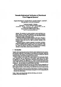
The general idea of the model checking approach is shown in Figure 1. The system under consideration is described in a specification language, usually a kind of process algebra. The specification is transformed into a representation, the semantic model, according to the semantic domain of the underlying process algebra. Properties to check are given by formulas of the specification logic, a logic like LTL, CTL or the µ-calculus. Model checking is testing whether the model satisfies the formula and in this way whether the underlying system fulfils the formulated property. Let us give a small example: Example 2.1 Suppose we want to specify a two element buffer. As a specific3
Semantic Domain for interpretation of specifiication and formulas, e.g. • Transition Systems • Petri Nets • Traces • ... in out out
τ
in
Abstraction/Specification of the Distributed System in a formal language like • CCS • ACP • Lotos • ...
Description of Properties in a logic like • LTL • CTL • µ-Calculus • LTrL • ...
Model Checking
(〈.〉 tt) ∧ (〈in〉 tt →
B1= in.out.B1 B2= (B1[out/i]||B1[in/i])\i
〈out〉 tt)
Figure 1: The idea of model checking systems ation language we use CCS [Mil89]. First we describe a one element buffer B1 by B1 = in.out.B1 which means that first the buffer makes an input action, then an output action and after that is in his originating state. Now we define the two element buffer by the parallel product of two buffers with capacity one. B2 = (B1 [out/i] | B1[in/i])\{i} Note that we substitute out by i and in by i (resp.) and restrict the communication over i to denote that this is an internal communication between the two buffers. The system is easier to understand when we look at its semantic model. We choose a transition system model. Its graphical representation is 4
τ
in
in out
out
A question is whether the buffer never deadlocks, i.e., is there always a possible next state? To specify this property we employ LTL. The corresponding formula is
2(3tt) meaning that always there is a next state such that true holds, i.e., that there is a next state. This question now can be answered by a model checking algorithm. Therefore, the important parameters of a model checking tool are concerned with the underlying notion of a distributed state or concurrency, the specification language and the specification logic. When we look at real systems we have the following side restriction which is known as “Lichtenstein-Pnueli” thesis [OA85]. The underlying system is large while the logical properties are small. Hence, when building a tool one needs to optimise the parameters according to the size of the system rather than to the size of the formula. However, a model checking tool has to reach more goals than just accepting the specification of the system and giving an answer of yes or no whether a formula is satisfied or not: It has to explain the specification given by the user in a (visual) way to give feed back. Furthermore, concerning the verification of formulae, the tool has to argue why a formula is satisfied or not. This allows the user to correct errors in the design. A simple no is not very helpful. So from the tool builder’s perspective, the parameters • models for the concurrent system • specification language • specification logic have to be discussed besides their use for model checking also wrt. the adequate visualisation. This is done in the next three sections. 5
3
An Overview of the Implementation of Truth
The verification tool Truth is developed by the modelling concurrent systems group at the University of Technology Aachen. Its aim is to serve as a prototype of a verification tool especially for testing new concepts for specification, modelling concurrency, logics and model checking algorithms. The main system is implemented using the functional programming language Haskell [Tho96] due to its declarative and easy to understand nature. In this way, the maintenance of the tool will become much easier. The name Truth was chosen because the main characteristic of a verification tool is that it tells the truth about the system.
3.1
The design of Truth
The architecture of Truth reflects the partition which was already shown in Figure 1. Is is partitioned into three separate major parts which deal with the different viewpoints of system verification. The overall structure of Truth is shown in Figure 2. We will now give a brief overview of the architecture and functionality of Truth. Further details will be given in the later section of this article. Truth is a tool for the verification of concurrent systems. Such systems can be specified in a process algebra, while properties for such systems can be expressed using a very expressive modal logic. The main task of Truth is answering questions of the form: Does specification Spec satisfy property Φ. We use Milner’s CCS as process algebra for the specification of concurrent systems. This gives access to a big number of real-life examples the system can be tested with. Also a lot of other verification tools support CCS specifications, hence we can compare the performance of Truth with tah of other systems. While CCS is a very popular choice it not necessary an optimal one for all application areas. This means that it is necessary to be able to replace CCS by a more appropriate choice depending on type of the system to be verified. Special care has been taken to minimise the influence of the choice of CCS on the rest of the implementation. Section 5 deals with this area in more detail. As we will argue in Section 4 the most crucial issue when building a verification 6
Specification Language
. . .
CCS
. . .
Semantic Domain
Graphical Simulation
LTS Annotations
Logic and Model Checking
LTS Data Structure
Misc. Analyses
µ-calculus Tableau Model Checker
Deadlocks
Graph. Output
Figure 2: Architecture of Truth tool, is the choice of the semantic domain. This choice has an overwhelming influence on the performance and usability of the tool. Currently we use labelled transition systems as the semantic domain. While these are well understood and are used in most tools, their use imposes a major limitation on the size of the system to be verified. To avoid the state space explosion, sharing of common data is performed via hashing. Also, the model is generated only on demand, for example, during the work of the model checking algorithm. In this way, errors of systems which are too large to be kept in memory can be detected as long as the error occurs in the first part of the system. While this doesn’t help to show that a system is correct it supports the user to improve the system. At the moment, BDDs are not used. It is planned to integrate a standard implementation for BDDs2 via the Greencard interface of the Glasgow Haskell Compiler in a future release. 2
for example, the one at http://www.cs.cmu.edu/~modelcheck/bdd.html
7
To visualise the specified system, the graph visualisation tool daVinci [FW94] is employed. The labelled transition system according to the specification given by the user is apparently a graph. Hence, the internal representation of the transition system is easily converted into a textual graph representation according to the syntax of the input language for daVinci. This string is send to daVinci which displays the corresponding graph using (on demand) a layout which minimises the number of edge crossings. Kozen’s µ-calculus is used as modal logic to express desired properties of the specified system. The expressiveness of the µ-calculus makes it ideal for such a task. Yet using the µ-calculus quickly leads to highly unscrutinizable formulae we add some syntactic sugar to make the use of the µ-calculus more convenient. Model checking is performed using the tableau based algorithm which was introduced by Cleaveland in [Cle90]. We currently work on the implementation of a game based model checking algorithm which we expect to perform much better then the one currently implemented. The implementation of the model checking algorithm is described in more detail in Section 6. In addition to these major components we have implemented a number of additional features which allow to examine the behaviour of the specified system. The most useful of these features probably is the graphical simulation of CCS processes. By separating a CCS process into a number of independently watched agents we are able to simulate a specified system in a much more structured and comprehandable way then this has been done by already existing tools. The simulation component will be especially useful to display model checking games. The implementation of Truth is described in full detail in [Tob98].
3.2
Implementation issues
Most of Truth is implemented in Haskell, are purely functional non-strict programming language [PH+ 96]. The declarative nature of this programming language as well as the total absence of side effects lead to an implementation, which is very well suited for extensions and change. This is one of the most fundamental requirements, the implementation had to meet. Some additional features make Haskell the ideal choice for our implementation. 8
3.2.1
Type system
Haskell is a strongly type language, i. e. every expression always can be assigned its type. At compile time a type checker checks the program for type consistency. This allows for the early detection of programming errors which speeds up the development process. It also makes the program more reliable. In addition Haskell has so called type classes, an elegant way to express overloading and integrate polymorphic functions into the program. Also a basic form of object oriented programming style is possible using these type classes.
3.2.2
Algebraic data types and pattern matching
Haskell supports the definition of algebraic data types. These are especially well suited to represent term structures, which we encounter at various places when implementing a verification tool. Together with pattern matching, we are able to express a number of algorithms in a very natural and hence very comprehandable way. We also use algebraic data types to implement abstract data types, which strengthens the modularity of our implementation.
3.2.3
Monadic IO
Until recently purely functional programming languages had trouble expressing input and output operations, which are side effects and hence can not easily be introduced into the languages. Monadic IO is a very elegant method to integrate input and output operations into purely functional languages [Wad97]. Haskell uses this concept and supplies versatile IO libraries which include exception handling and file manipulation.
3.3
The Glasgow Haskell compiler
The Glasgow Haskell compiler (GHC) is a highly optimising compiler for Haskell which can create binary executables for a number of hardware platforms [JHH+ 93]. Unlike many other implementations of functional languages which translate programs into an interpreted byte code, the GHC translates into native machine code. This leads to very good run time performance of the compiled programs. 9
Compilation into machine code is performed using GNU C as an intermediate language which allows the use of all optimisations the GNU C compiler applies to its input. In addition to the normal Haskell libraries, the GHC supplies a number of additional features which are very useful to get an efficient implementation.
3.3.1
State monads
While purely functional programming languages are capable of expressing some algorithms very briefly and efficiently, they have problems with expressing certain other algorithms. Especially graph algorithms which make use of the explicit sharing of substructures cannot be implement in purely functional languages in an efficient way. The same applies to hash tables which have to be updated several times during the runtime of a program. State monads [LJ94] are a way of expressing destructive updates of data structures in a safe, i. e. referentially transparent way. To do this computations are build up like scripts which are then applied to a state space. We use state monads to implement efficient hash tables and to store and process transition systems.
3.3.2
Additional libraries
The GHC supplies several high quality implementations of common data structures. We only want to mention the fast implementation of sets and of finite mappings, which are used almost throughout the whole implementation of Truth. Also the implementation of a Posix compliant library to access the UNIX operating system has proven to be very useful for implementing a usable system.
3.3.3
Additional features
There is a number of features of the GHC Haskell system which have not be used in the current implementation of Truth but which will be useful when extending the system. Especially the Greencard system which allows the calling of arbitrary C functions from within Haskell will be used to implement efficient 10
BDD based storage of transition systems. Parallel Haskell might be used for a high level implementation of distributed model checking algorithms and so on.
3.4
Java
There are several libraries to implement graphical user interfaces with Haskell. Yet these libraries can only be considered to be alpha versions and they have not proven to be usable when we tried to implement the graphical simulation of CCS processes. As an alternative we chose Java, which has a powerful library for the development of graphical user interfaces. It also allows easy porting of our system to different platforms because programs are not compiled into native machine code but into abstract byte code. The interpretation of this code is done by abstract machines which are available for nearly every hardware platform. Since our user interface has neither high speed nor high memory demands, this approach is suitable for Truth.
4
Models for Concurrency
The most important question is to choose the adequate model for concurrency. Several proposals have been given and were analysed during the last 20 years. To name a few: Transition systems, Petri nets, Mazurkiewics traces, event structures. In [SNW96] several models are compared on a formal basis. In this section, we pick up the proposed taxonomy and discuss the consequences for model checking tools. The common idea of all models is that they are based on atomic units which are indivisible and constitute the steps out of which computations are built. They differ in the level of abstraction from the underlying system. For example, so called interleaving models reduce concurrency to interleaving. In this way they abstract from true concurrency and postulate that the concurrent execution of two actions a and b are equivalent to the execution of a and then b or b and then a. The full classification according to [SNW96] is as follows: 11
synchronisation trees
labelled event structures
Behaviour Hoare languages
deterministic labelled event structures
System
transition systems with independence
transition systems
Branching Linear deterministic transition systems Interleaving
deterministic transitions systems with independence Noninterleaving
Figure 3: Examples of models for concurrency behaviour model linear time model interleaving model
– system model – branching time model – noninterleaving model
Note that the parameters are orthogonal so that there are eight categories of models. Furthermore, for each category a well known theory of concurrency can be given. As an example we refer to the cube shown in Figure 3.
4.1
Behaviour versus System Model
The first classification is according to whether the model describes the underlying system or it concentrates on its behaviour. In the context of verification of concurrent systems, the user specifies the system with the help of a specification language. This usually has a natural system model. For example, CCS terms have an easy to understand transition system semantics. Concerning the visualisation of the specification, a system model is more appropriate because it reflects the user’s view. For model checking, as we will see in Section 6.1, the behaviour of the system is considered. For example, for transition systems, either the set of all runs of the system or one tree in which every path represents a run, is analysed depending on the applied logic (LT L or CT L). However, in general the behaviour of the 12
system is an infinite object (every run is usually infinite). Hence, from the tool builder’s perspective, the internal representation of the specification needs to be a system model, or in the case of infinite state systems3 ([Bur97]), even only a finite description of the system model. Model checking algorithms have to analyse the system model wrt. its behaviour.
4.2
Linear Time versus Branching Time Model
When we restrict to system models, in linear time models the next state of a system is determined by the current state and an atomic event. Branching time system models, on the contrary, have several possible next states. They are more natural for describing systems as the complexity of specifying large systems is reduced if nondeterministic constructs in the design notion are supported. However, the situation is different when we look at the behaviour of the system. For model checking, often the linear behaviour of the system is important. Which kind of sequences can an observer of our system recognise? As linear time versus branching time is only relevant for model checking, we postpone the discussion to Section 6.1.
4.3
Interleaving versus Noninterleaving Model
The most important question regarding modelling concurrent systems is whether an interleaving or noninterleaving model should be preferred. In an interleaving model, the concurrent occurrence of two events is modelled via their nondeterministic interleaving. Hence, the analysis of concurrent systems is reduced to the analysis of nondeterministic sequential systems. This reduction was important for the success of formal methods because well known theories, e.g., the theory of nondeterministic finite automata, could be applied for verification tools. However, interleaving models have a big disadvantage, the huge state space. The problem can easily be understood looking at the following example. Let a and b be two actions of our system which are independent on an intuitive basis. This usually leads to a specification stating that a and b can be executed concurrently because the user wants to abstract whether a and b are executed in a precise 3
where already the system model is infinite
13
order. In the interleaving model, the independence of the two actions is ignored. Instead, the system consists of states representing all possible interleavings, a number which is exponential in the number of the concurrent independent actions. As the systems under consideration are usually large this model is not adequate. Furthermore, the visualisation of an interleaving model is less intuitive for the user because usually he describes the underlying system by defining local parts of the system and their interaction. Hence, he expects this view of the system to be visualised with the help of his tool. On the contrary, most current model checking tools employ interleaving models ([Pri96]). But much effort is spent for developing the theory of noninterleaving models (such as Mazurkiewics traces [DR95]) and corresponding logics and model checking algorithms. However, for the development of model checking tools for todays industrial usage an interleaving model should be preferred due to its well understood theory. Moreover, several techniques have been developed to improve the benefit of interleaving models, that means, to avoid the state space explosion problem. The most important is known as Symbolic Model Checking ([McM93]). The basic idea is to describe the underlying (transition) system by a boolean function which can be coded efficiently via binary decision diagrams (BDDs, [Bry85]). The boolean function is represented as a graph in which common subgraphs are shared. Especially for modelling hardware and hardware-like systems the average state space is reduced dramatically. The use of symbolic model checking techniques proved that model checking can be used for real systems and not just for toy examples. For the rest of the paper, we concentrate on finite state labelled transition systems as a model for concurrency.
4.4
Implementation issues
As argued in the previous subsection, Truth only supports labelled transitions systems as the semantic domain (at this time). Special care has to be taken in order to get an efficient implementation, especially when using a purely functional implementation language like Haskell. The Labelled Transitions System (LTS) component component of Truth supplies a very limited functionality on which further analysis steps like model 14
checking are built. A further constraint is added, because we want to use a local model checking algorithm. To exploit the advantages of a local method the LTS has to be built in a demand driven manner. This way only the part of the transition system which is relevant for a given formula has to be built up. This can lead to enormous speed ups of the model checking process. Since we want to support not only model checking but several other (graph based) analyses of the transition system, we must aim for a very generic implementation. Since all these analyses (including model checking) work by traversing the LTS while annotating it, we give special support for this behaviour. By using mutable data structures we are able to update the transition system in constant time. This is a necessary property of the data structure if we want to get an efficient implementation, because building and analysing the LTS is the core functionality of any modelchecker. To detect cycles during the generation of the transition system we use a hash table to map process terms to the vertices of the LTS. We cannot use the terms as states of the LTS since our implementation relies on a array structure to express sharing within the LTS. Terms cannot be ordered in a way that would make them suitable to act as indices for an array. All these functions are encapsulated in a monad to make the LTS functionality as easy to use as possible. Using this monad very concise implementations of different analyses are possible. Here is an example. The following fragment of Haskell code inspects a LTS for deadlock states, i. e. states which do not have an outgoing transition. 1 findDls::ProcEnv->[Action]->LTSState->LTS_M s Bool [Derivative] 2 findDls penv accu st 3 = ifLTS ( getAddLabelLTS st ) 4 ( returnLTS [] ) 5 ( expandLTSState penv st ‘thenLTS‘ \ succs -> 6 case succs of 7 [] -> getLabelLTS st ‘thenLTS‘ \ proc -> 8 returnLTS [(reverse accu,proc)] 9 somesuccs -> 10 let 11 next_step (act,states)
15
12 13 14 15
= mapConcatLTS (findDls penv (act:accu)) states in mapConcatLTS next_step somesuccs )
The function exspects several parameters: A process environment which is used to expand states of the LTS, a list of actions which label the path to the considered vertex and the vertex to be considered. It returns a list of deadlocked states and pathes to these states. Line 3 checks if the considered vertex has been visited before. If this is the case (line 4) we return an empty list since no new deadlocks have been found. If the vertex has not been visited before we have to generate its successors. This is done by the call to expandLTSState in line 5. This function expands the transition system for this vertex and returns a list of all the successors of the vertex st. If st has no successors (line 7) we have found a deadlock, so we add the path and the process term which labels st to the result list (line 7,8). Otherwise we recursively call findDls for all successors of st and combine the results into a single list (line 12,14). As we desribed above, labelled transition systems are not an optimal choice for modelling the behaviour of a concurrent systems. We aim to replace them in the future by a semantic model which can model concurrency on a higher level and hence will not have the state explosion problem. Still the existing implementation can serve as the basis for this more advanced implementation, because (nearly) all semantic models have a graph-like structure. The states may have a more strucutred content and the edges may be labelled not by actions but by sequences of actions — still we are dealing with a graph-like structure which will have to be stored. For this the existing data strucures are an ideal foundation.
5
Specification Languages
The situation for specification languages is much more difficult than for models for concurrency. There is a large number of different specification languages, new languages occur and existing change rapidly. 16
If one looks for a taxonomy of specification languages further problems arise. Some attributes for specification languages are for example: • time • mobility • data values • probability • ... But, neither the list is complete nor the items characterise the language in a binary way. For example, for time, one can distinguish between no time, real time, discrete time, urgent time, time deadlocks and possible other notions of time. Similar problems arise for the other attributes, for example, no values, finite values, infinite values, . . . However, from the tool builder’s perspective, the situation for specification languages is not such sobering: The first step in the design of a verification tool is to select the favourite notion of concurrency as described in the last section. This limits the number of specification languages because it is obvious that the specification language’s semantics has to be according to the semantic model. In some sense also the converse is true: If the specification language’s semantics is according to the semantic model and if its semantics can be described by a finite number of rules it is easy to adopt the specification language for the underlying verification tool. Let us explain the last sentence by an example. Let us consider finite transition systems as our intended model. Many specification languages have a transition system based semantics, for example CCS ([Mil89]), CSP ([Hoa85]), LOTOS ([BB89]) or the π-calculus ([MPW93]). Note that LOTOS includes the specification of values and the π-calculus supports specifying mobility of processes. As model checking works on the semantics of the specified system rather than on the specification one can abstract for model checking from the underlying process algebra as long as a semantic function can be provided yielding the semantic model in some internal representation. Concerning visualisation, usually the specified model (transition system) is shown rather than the specification. Hence, from 17
Specification Language Compiler Specification Language Description
Truth Frontend Syntax Analyser
Syntax
Semantics
Semantic Analyser
Parse functions
Semantic functions
Figure 4: Overview of Process Algebra Compiler
the tool builder’s perspective, a modification of the underlying process algebra means changing the parser and some kind of semantic function. Moreover, in a wide range of cases the semantics of the specification language can be described in a uniform way. For example, the languages mentioned above have in common that their semantics can be denoted by SOS-rules [Plo81]. This opens the possibility to develop more generic verification tools. Instead of developing a parser and a corresponding semantic function one develops a process algebra compiler reading a process algebra description consisting of a specification of the syntax of the process algebra and its semantics denoted via SOS-rules. The process algebra compiler generates a front end for the verification tool consisting of a parser and a corresponding semantic function according to the SOS-rules. These functions are linked to the rest of the verification tool and that’s it. This approach was studied in [CMS95] where details of the design can be found. It was shown that applying this technique even efficient tools can be generated. Figure 4 gives a schematic overview of a process algebra compiler. Currently, we are extending this approach to a wider class of specification languages by mentioning a uniform operational semantics for concurrent systems covering more cases than these where SOS-rules are applicable. This approach will be implemented for the verification tool Truth. When we concentrate on transition system based semantics we conclude by emphasising that from the tool builder’s perspective already today the adoption of new specification languages or the modification of languages can be handled in more or less inexpensive way by developing generic tools. Hence, usually you will develop a generic tool with a some specification language and will modify your language during the employment of the tool due to the needs of the user and the underlying system to be specified. 18
5.1
State of the implementation
As a first choice we implemented CCS support for Truth. This choice was motivated mainly by the number of existing CCS specifications which are available. By supporting CCS specifications in Truth we were able to access a big number of test specifications and to compare the performance of Truth to that of other existing tools. There are three major constraints on the implementation of the CCS component our implementation had to meet: 1. The influence of the choice of CCS as specification language has to be minimised. 2. To get an efficient tool, the calculation of the successor relation of process terms had to be as fast as possible. 3. The size of the term representation has to be as small as possible. In the remaining part of this section we desribe the measures we undertook to meet these three goals. 5.1.1
Minimising the influence
As the choice of the specification language is highly dependent on the problem domain and the system to be specified, number 1 has the highest priority. Fortunately 1 is also easy to meet since most specification languages use the same abstractions. System states are desribed by terms in some specification formalism. These terms fully describe the global state of the system. From this state susccessor states can be generated which again are described by terms. Using this abstraction it is easy to derive a general interface which most specification formalism can easily be fitted into. We only require the implementation of the specific specification formalism to supply basic types Process and Action together with two storage types (ProcEnv, ActEnv) which capture the definitions read from an input file. Except from some functions for parsing and printing of definitions as well as for reading and writing the storage types the implementation only has to provide 19
a single function (transitions) which maps as Process two its successors according to the transition function of the specification formalism. This interface seems simple enough that it can be filled by an automatically generated module which could be provided by a process algebra compiler. 5.1.2
Towards an efficient implementation
To meet goal number 2, transitions does not simply have the type transitions::ProcEnv -> Process -> [(Action,[Process])]
but a type which is slightly more complicated: transitions:: ProcEnv -> Process -> ProcSuccsHT s -> SST s ProcSuccs
We add a hash table to the arguments of the function. This hash table is used to store computations of successors of process terms which have been performed at an earlier time. To use an efficient implementation of a hash table we have to embed the comutation into a state monad, hence the strange return type SST s ProcSuccs. Yet the additional complexity of adding the hash table proves to make the calculation of the successor relation much more efficient as is shown by the figures in the following table show. They state the time Truth took to generate the whole transition systems induced by various examples. We considered the following examples: Knuth 802 Mailer ATM 3LN
An solution of the mutual exclusion problem by Knuth. A part of the implementation of the data link control layer according to the IEEE 802.2 standard. A specification of an email system which has been used at the Edinburgh university. A specification of the connect phase of two ATM switches. Three instances of the alternating bit protocol forming a single channel.
We tested five different generation algorithms/tools: 20
Knuth 802 Mailer ATM 3LN
Naiv 0.28 s 0.58 s 3.31 s 4.84 s 131.43 s
Hash 0.27 s 0.47 s 3.35 s 13.15 s 94.21 s
H/F 0.28 s 0.43 s 1.60 s 1.41 s 52.22 s
NCSU 0.33 s 0.63 s 3.48 s 3.54 s 59.07 s
CWB 0.80 s 2.20 s 4.24 s 2.50 s 74.50 s
Table 1: Runtime of LTS geneation Naiv
A simple implementation without the use of hash tables to store precalculated successors. Hash The algorithm with hashing. H/F The algorithm with hashing and tree flattening, an additional optimisation which will be described later on. NCSU The NCSU concurrency workbench. CWB The Edinburgh concurrency workbench, version 7.1β.
The test were run on an Ultra Sparc station running Solaris 2.5 with 512 MB of main memory. Tree flattening was introduced into the algorithm after we noted that in certain cases hashing actually slowed down the generation of transition systems down. An inspection of the runnig program with a profiler showed, that Truth spent most of its time comparing process terms to solve clashes of the hash function. This was especially slow in the presence of big relabelings and restrictions. Tree flattening allows to speed up this task significantly and leads to the good runtimes shown in the column labelled H/F.
5.1.3
Space issues
Also memory consuption of the algorithms are an important property. We tested the memory consumption of Truth with the same examples. The results are shown in the following table. Unfortunately it was not possible to get exact values for the memory consumption of the concurrency workbenches since the ML runtime system (both were implemented using ML) does not allow for an easy extraction of those values. The figures shown for Truth are the maximum 21
Knuth 802 Mailer ATM 3LN
Naiv 0.5 MB 0.56 MB 1.16 MB 1.47 MB 15.04 MB
Hash 1.12 MB 1.34 MB 3.14 MB 2.25 MB 30.78 MB
NCSU 47.8 MB
CWB 148.5 MB
Table 2: Memory consumption of LTS generation. heap resedency, i. e. the largest sice of the heap after a garbage collection. The figures for NCSU and CWB are the maximum size of the UNIX process. As can easily be seen, hashing about doubles the memory consumption of the algorithm. This is due to the large memory consumption of the hash table itself. Still our implementation performs very well when compared to the concurrency workbenches. Tree flattening does not significantly change the memory demand of the algorithm hence it is not shown sperately in the table.
6
Specification Logics
Recall from Section 2 that in the model checking approach for verification the properties to be checked are expressed as logical formulas. Typical properties are safety, liveness and fairness properties [Eme96]. A safety property denotes that some “good” property ϕ always holds. Safety properties are important for critical systems. Liveness formulas describe that some property ϕ will always have the possibility to hold sometime. For example, regardless which state a server reaches it should always have the possible to reach a state where it accepts a new request. Fairness properties describe that the behaviour of the system is fair wrt. resources or processes. There are several notions of fairness, e.g., some property ϕ holds infinitely often for every execution which is also called unconditional fairness. Properties are usually expressed using temporal logics [Sti96]. It is clear, that the semantics of the logic has to be in some sense according to the semantic 22
model. Hence, there are several logics depending on the (system) model. Furthermore, logical formulas usually describe the behaviour of the system. Hence, given the system model one has the freedom to define what he understands by its behaviour. For example, in the case of transition systems, the behaviour of the system can be understood by a set of all possible runs of the system or by a tree in which every path denotes a run of the system depending on whether you prefer a linear behaviour model or a branching behaviour model. Moreover, similar to the case of specification languages, there are several logics which are interpreted over the same class of models differing in expressiveness and complexity of the model checking problem. For transitions systems, the most important logics are LTL ([OA85]), CTL and CTL* ([ES88]) and the µ-calculus ([Koz83],[Eme97]). Linear Time temporal Logic (LTL) is interpreted over the linear behaviour model generated by the underlying transition system. Hence, a formula describes a property of a single run of the system. To determine a property of the system, one usually identifies the system with all possible runs of the system and looks for a run not satisfying the property. The system fulfils the property whether or not such a run could be found. Errors in the design can easily be visualised because if a property is not valid a run must exist which violates the property. Presenting this run, the user can understand the wrong behaviour of the system. Safety properties can easily be expressed in LTL. For liveness and fairness the situation is more difficult. Suppose that a system can evolve in some state q and then can but needn’t reach a state q ′ . This means that a corresponding safety property is satisfied. However, if one looks at every sequential run of the system one can observe runs where q is followed by q ′ and runs where q is not followed by q ′ . As in linear time models one only speaks about all or no runs this property can’t be expressed in LTL. Also, some notions of fairness can’t be expressed for the same reasons. Computation Tree Logic (CTL) and CTL*, an extension of CTL, are interpreted over the branching behaviour model generated by the system. Hence, a formula describes a property of the whole tree of computations of the system. However, via the modalities of the logic several paths can be selected. The visualisation of errors is more complicated because an error identifies a subtree of the tree of all executions violating a certain property, but neither a tree nor its 23
Lµ
Lµ3 Lµ2 CTL* Lµ1
LTL
CTL
Figure 5: Expressiveness of logics
contained runs are easy to visualise. However, visualisation is possible in an interactive way if a certain model checking technique is used. This is described in the next subsection. It is easy to express safety and liveness formulas in CTL. However, CTL is relatively simple, e.g., unconditional fairness is not expressible but it is expressible in CTL*. The µ-calculus, however, is interpreted directly over the transition system (the system model). It is a fixpoint logic describing sets of states with a certain property. Usually one considers a property ϕ to be satisfied by the system iff the initial state of the system has the property ϕ, hence, iff the initial state is a member of the set of states satisfying ϕ. To define sets of states, least fixpoints and greatest fixpoint modal quantifiers can be used. The µ-calculus is a very expressive logic and several sub logics, denoted by Lµk depending on the alternation depth of fixed points k, are studied. Intuitively, the alternation depth refers to the depth of nesting of alternating least and greatest fixpoint quantifiers. It can be shown that formulas of LTL and CTL can be transformed into formulas of Lµ1 exponential and linear (respectively) in the size of the original formula. CTL* formulas can be transformed into Lµ2 formulas. In [Bra96] it was shown, that the hierarchy Lµk for k ∈ IN is strict for infinite models, i.e., at least for infinite models, more alternation leads to more expressive power. Figure 5 summarises the expressiveness results mentioned above. However, 24
logic
complexity class
time complexity of known algorithms
LTL CTL CTL* Lµk
PSPACE complete P complete PSPACE complete NP ∩ co-NP
O(|M| · exp(|ϕ|)) O(|M| · |ϕ|) O(|M| · exp(|ϕ|)) (|M| · |ϕ|)O(k)
Table 3: Complexity of logics
expressiveness can’t be considered isolated from the complexity of the model checking problem. Intuitively, it is clear that more expressiveness leads to a higher complexity. Table 3 (taken from [Eme96]) gives an overview of the complexity for the model checking problem for the logics described above. The underlying transition system is denoted by M and the property by ϕ. We see that known model checking procedures for the full µ-calculus are exponential in the size of the alternation depth. Hence, the expressive power is paid by a high complexity. While this is true also for CTL*, experience shows that typical4 CTL and CTL* formulas are usually shorter than equivalent µ-calculus formulas. However, we think that in a verification tool the implementation of two algorithms would be the best idea, a fast algorithm for CTL formulas and one for the µ-calculus since most typical formulas are expressible in CTL and CTL* formulas can be translated to formulas of the µ-calculus. In this way nearly every logic is easily supported.
6.1
Model Checking
Model checking answers the question whether a given formula is satisfied by the specified model. A simple answer whether a formula is valid or not is enough in theory. However, from the tool builder’s perspective, the way of determining the answer needs to be considered, too. Two important attributes for model checking algorithms can be discussed, global or local model checking and its underlying mathematical theory. 4
in the context of verification
25
6.1.1
Global versus Local Model Checking
The general question for model checking is whether some kind of initial state of a system satisfies a given formula ϕ. Of course, the answer depends on the specified system (at least if we restrict to interesting formulas). Hence, one way to answer the question is: 1. read specification 2. generate model (e.g., a transition system) 3. determine semantics of formula and check whether it is satisfied or not This approach is called global model checking because the model checking algorithm works on the total system. But for the verification of large systems this has a big drawback, the whole system has to be kept in memory. Often, formulas speak only of parts of the system, such as if the system reaches some state q than later on it will reach a state q ′ . Hence, if a system can evolve in q only states which are reachable from q must be considered. In the local model checking approach the underlying system is constructed on demand. While in the worst case also the total system has to be generated and to be kept in memory, in the average case parts of the system suffice. In this way, even systems to large to be kept in memory can be analysed and (partly) debugged. Hence, local model checking algorithms should be preferred for verification tools. For the logics mentioned above 6 local model checking algorithms exist [GPVW95, BC96, SW91, Sti95, Sti97]. 6.1.2
Theoretical basis of model checking algorithms
Three approaches for model checking algorithms can be distinguished • automata based • tableau based • game based 26
Automata based The underlying system M is transformed into a corresponding automaton AM accepting all behaviours of the system. The property ϕ is negated and an automaton A¬ϕ is constructed accepting all satisfying models of ¬ϕ. Next, the intersection automaton AM∩¬ϕ of AM and A¬ϕ is constructed. If the language accepted by AM∩¬ϕ is not empty there is a behaviour of the system satisfying ¬ϕ, hence, violating ϕ. In this way, model checking is reduced to automata theory. For interleaving system models, if the intended behaviour model is a linear model, the corresponding automaton is a (B¨ uchi) automaton over words and if the intended model is a branching behaviour model the corresponding automaton will be a tree automaton. The advantage of the automata based approach is that the automata AM∩¬ϕ , AM and A¬ϕ can usually be constructed on demand while testing the emptiness of the language of AM∩¬ϕ . Hence, the arising algorithms are local. Furthermore, if the behaviour model is linear and the formula is not satisfied every word in the language of AM∩¬ϕ is a counterexample and can be shown to the user. While an analogon is also true for branching models it is much more difficult to visualise a tree. Note that this method is only applicable iff the satisfiability problem for the logic is decidable because a formula ϕ is satisfiable iff the language of Aϕ is not empty. Automata based model checking algorithms are described in [Var96] (for LTL) and in [VBW94] (for CTL).
Tableau based Tableaus are usually used to show the satisfiability of formulas. One tries to construct a tree with good leafs corresponding to a given formula according to the tableau rules. If such a tree exists, the formula is satisfiable [Fit93]. For model checking the tableau rules are modified to take the corresponding system under consideration. In this way, a good tableau is constructed iff the formula is satisfied by the specified model. Tableau based model checking algorithms are usually local model checking algorithms because the root of the tree is formed by the formula and the initial state of the system. While constructing the tree further states of the system are generated. Furthermore, as the tree is build in a depth first manner only one path has to be kept in memory at a time. 27
For the visualisation, similar restrictions as in the case of automata hold, since it is not clear how describe that there is no good tree. A tableau based model checking algorithm for CTL is described in [Eme96], one for the µ-calculus is described in [Cle90]. Game based In the game based approach, the board of the game is build upon the formula and the system and is played by two players, Player I and Player II. Player I tries to show that the formula is not valid while Player II tries to show the contrary. One of the two players has a winning strategy, that means he can win the game regardless of how the other plays. Of course, Player I has a winning strategy if and only if the formula is satisfied by the transition system. Hence, the job of a model checking algorithm based on games is to check which player has a winning strategy. Usually the game based approach yields a local algorithm since the game starts in a state corresponding to the formula and the initial state of the system. While trying different moves the system is generated. The game based approach has some advantages. First we think that it is easier to understand than the other approaches. Furthermore, regardless whether the formula is satisfied or not, a winning strategy is found and can be used to explain why a formula is valid or not. If the user doesn’t believe the tool he can analyse the specified system wrt. the formula while playing against the tool. Although if he will loose he will understand why. The game based approach and a model checking algorithm for the µ-calculus are described in [Sti97] and are implemented in the current version of the CWB.
6.2
State of the implementation
At the moment we are working on the implementation of a game based model checking algorithm and to implement this algorithm in Truth along with the possibility to play games against Truth in a graphical way. Until this is finished, Truth is using a tableau based model checking algorithm derived from the algorithm described in [Cle90]. It is a local algorithm which brings the advantages described earlier in this section. We have run several test to compare our implementation to several existing 28
NCSU
Truth Φ1 Φ2 Φ3 Φ4 Φ5 Φ6
73.16 s 0.11 s 598.52 s 187.82 s 0.14 s out of mem.
34.78 MB 0.48 MB 133.55 MB 92.50 MB 0.47 MB -
64.99 67.91 73.66 78.23 85.72 n.a.
s s s s s
147.49 MB 148.87 MB 151.12 MB 148.43 MB 155.62 MB n.a.
CWB 75.54 s 0.13 s 99.37 s 87.76 s 0.12 s 0.16 s
153.30 MB 196.82 MB 180.13 MB -
Table 4: Runtimes of the model checker tools. Some results of these test are shown below. Several formulae were tested over the 3LN transitions system. Φ6 lies outside the fragment of the µ-calculus the NCSU concurrency workbench can handle hence we could not test the performance in this case. It is clear to see that local algorithms sometimes have a much smaller runtime then the global one of the NCSU concurrency workbench. This is especially obvious in the case Φ5 where both Truth and CWB only take fragments of a second to come up with an answer while the NCSU concurrency workbench takes more then a minute. It is also obvious that the game based model checking algorithm CWB uses is inferior to the tableau based algorithm currently implemented in Truth. This is reason we are working on an implementation of a game based model checking algorithm in Truth.
7
An example: The alternating bit protocol
This last section will give an example of the application of Truth to a small specifiaction. It will give you a quick start to use Truth as a verification system. Network protocols are typical examples for concurrent systems. A whole class of protocols deals with tranmission of data using unreliable channels. An unreliable channel may loose message, duplicate or corrupt them. In our example we consider channels which guarantee a single transmission of any message, yet they may corrupt the message during the transmission. Things are even more complicated by the fact that also the chanell use to send acknowledgements may corrupt these messages. 29
A well-known example for transmission over such channels is the alternating bit protocol [Mil89], short ABP. It uses a single bit to control transmission in a way that initiates a retransmisson of the last message in case of an error. The two channels are modelled using CCS in the following manner: K = sendreq0 .(send0 .K + send⊥ .K) + sendreq1 .(send1 .K + send⊥ .K) L = ackreq0 .(ack0 .L + ack⊥ .L) + ackreq1 .(ack1 .L + ack⊥ .L) After receiving a sendreqi message, K can either transmit this message and perform a sendi action. It may also corrupt the message and transmit a send⊥ . L is modelled analogously. This example nicely shows how we abstract from the original system. Neither the content of the messages is modelled nor the error detection mechanism. This has no influence on the protocol and hence is not taken into account. Sender and receiver use this single bit to ensure correct transmission even in case of errors. The specification of the sender and the receiver is a bit more complicated. It is shown in Figure 7 using the Truth syntax for CCS. A schematic view of the system can be found in Figure 6. Sender and receiver use the actions input and output to communicate with the world to accept messages for transmission and to signal the correct transmission of a message. In addition to the specification we want to define some properties the system should satisfy. These must be stated as formulae of the µ-calculus for Truth. A usual requirement for a concurrent system is, that it will never reach a deadlock state, i. e. a state in which the system cannot perform any more actions. A formula which states that there is no reachable state in which outgoing transitions exist, is for example: NoDeadlock := AG(h−itt) ≡ νX.h−itt ∧ [−]X The ABP will contain a livelock situation if there is a reachable state of the system from which there exists an infinite path which is labelled only with τ actions. A formula stating that no such state exists is for example NoLivelock := AG(¬νX.hτ iX) The ABP can accept messages for transmission if it can perform an input step or if there is a finite sequence of τ steps which lead to a state in which an 30
Sender
input
ack 0
sendreq 0 sendreq 1
ack bottom ack 1
K
send 0
L
send bottom send 1
ackreq 1 ackreq 0
Receiver
output
Figure 6: A schematic view of the ABP input step is possible. CanInput := µX.hinputitt ∨ hτ iX Analogously we can express that the system can output a message. CanOutput := µX.houtputitt ∨ hτ iX The system is working if at any time one of the above formulae holds. Operating := AG(CanInput ∨ CanOutput) Another important property is, that no message is output twice. NoRepeat := AG([input]¬CanInput ∧ [output]¬CanOutput) In Truth the according formulae have the following syntax: prop AG(P) = max X.P && [-]X prop NoDeadlock = AG(tt) 31
def def def def def def def def
ABP = (Sender | K | L | Receiver) \ Internal Sender = S_0 S_0 = ’input.S_0’ S_1 = ’input.S_1’ S_0’ = sendreq_0.S_0’’ S_1’ = sendreq_1.S_1’’ S_0’’ = ’ack_0.S_1 + ’ack_1.S_0’ + ’ack_bottom.S_0’ S_1’’ = ’ack_1.S_0 + ’ack_0.S_1’ + ’ack_bottom.S_1’
def Receiver = R_0 def R_0 = ’send_0.output.ackreq_0.R_1 + ’send_1.ackreq_1.R_0 + ’send_bottom.ackreq_1.R_0 def R_1 = ’send_1.output.ackreq_1.R_0 + ’send_0.ackreq_0.R_1 + ’send_bottom.ackreq_0.R_1 def K = ’sendreq_0.(send_0.K + send_bottom.K) + ’sendreq_1.(send_1.K + send_bottom.K) def L = ’ackreq_0.(ack_0.L + ack_bottom.L) + ’ackreq_1.(ack_1.L + ack_bottom.L) def Internal = { sendreq_0, sendreq_1, send_0, send_1, send_bottom, ackreq_0, ackreq_1, ack_0, ack_1, ack_bottom } Figure 7: The specification of the ABP
32
prop prop prop prop prop
NoLivelock = AG(max X.X) CanInput = min Y.tt || Y CanOutput = min Y.tt || Y Operating = AG (CanInput() || CanOutput()) NoRepeat = AG ([’input](~CanInput()) || [output](~CanOutput()))
Consider these definitions in a file ”abp”. The following is an example session with Truth. ________________ / / Lehrstuhl II fuer Informatik ___ ___ And /_____ _____/ RWTH Aachen / / / / / / ____ __ __ _______ / / / / nothing / / / _ \ / / / / /__ __/ / /____/ / / / / |_| | / / / / / / / / but / / / _ _/ / / / / / / / _____ / / / / / | | / / / / / / / / / / the / / / / | | / \__/ / / / / / / / /____/ /_/ |_| \______/ /_/ /__/ /__/ 0.9 Martin Lange, Martin Leucker, Stephan Tobies (Version 0.9 --- February 1998) - ENJOY! truth> file abp
Truth comes up with a status message and prompts for an input. By typing ”file abp” the file with the definitions is loaded into the system. truth> size ABP The process ABP has 23 states and 28 transitions. The command size gives a first idea of the size of the specified system. With 23 states we are dealing with a very small system. truth> plot Sender truth> plot K truth> plot ABP The command plot creates an output of the transition systems which are induced by the different process terms. Transition systems are displayed using the daVinci graph visualization tool. An example of these outputs can be found in Figure 8 and 9. The tableau based model checker is initiated with the command tab. Testing the various formulae yields the follwing output. 33
Sender
’input
S_0’
sendreq_0
S_0’’
’ack_bottom
’ack_0
K
’ack_1 ’sendreq_0
’sendreq_1
send_0.K + send_bottom.K
send_1.K + send_bottom.K
S_1
’input send_bottom
send_0
send_bottom
send_1
S_1’
sendreq_1
S_1’’
’ack_bottom
’ack_1
’ack_0
S_0
’input
Figure 8: Output of transition systems with daVinci truth> tab ABP NoDeadlock TRUE, the process satisfies truth> tab ABP NoLivelock FALSE, the process does not truth> tab ABP Operating TRUE, the process satisfies truth> tab ABP NoRepeat TRUE, the process satisfies
the formula satisfy the formula the formula the formula
The model checker states that NoLivelock is not satisfied by ABP . A quick examination with the graphical simulation confirms this. Before starting the simulation we divide ABP into sperately watched agents using ”#” as a a parallel composition operator which indicates the units of this decomposition. truth> def SimABP = (Sender # K # L # Receiver) \ Internal 34
ABP
’input
(S_0’ | K | L | Receiver)\Internal
tau
(S_0’’ | (send_0.K + send_bottom.K) | L | Receiver)\Internal
tau
tau
(S_0’’ | K | L | ackreq_1.R_0)\Internal
tau
(S_0’’ | K | (ack_1.L + ack_bottom.L) | R_0)\Internal
tau
(S_0’ | K | L | R_0)\Internal
tau
(S_0’’ | (send_0.K + send_bottom.K) | L | R_0)\Internal
tau
tau
(S_0’’ | K | L | output.ackreq_0.R_1)\Internal
output
(S_0’’ | K | L | ackreq_0.R_1)\Internal
tau
(S_0’’ | K | (ack_0.L + ack_bottom.L) | R_1)\Internal
tau
tau
(S_1 | K | L | R_1)\Internal
(S_0’ | K | L | R_1)\Internal
’input
tau
(S_1’ | K | L | R_1)\Internal
(S_0’’ | (send_0.K + send_bottom.K) | L | R_1)\Internal
tau
tau
(S_1’’ | (send_1.K + send_bottom.K) | L | R_1)\Internal
tau
tau
(S_1’’ | K | L | output.ackreq_1.R_0)\Internal
(S_1’’ | K | L | ackreq_0.R_1)\Internal
output
tau
(S_1’’ | K | L | ackreq_1.R_0)\Internal
(S_1’’ | K | (ack_0.L + ack_bottom.L) | R_1)\Internal
tau
tau
(S_1’’ | K | (ack_1.L + ack_bottom.L) | R_0)\Internal
tau
tau
(S_0 | K | L | R_0)\Internal
(S_1’ | K | L | R_0)\Internal
tau
daVinci
V2.0.3
’input
(S_1’’ | (send_1.K + send_bottom.K) | L | R_0)\Internal
tau
Figure 9: The ABP transition system 35
truth> sim SimABP
Figure 10: Simulation of the ABP
If a channel always corrupt the transmitted message this will lead to a τ cycle. Figure 7 shows this cycle. In the bottom row the system has the same state as in row 2. The system now may perform this cycle infinitely often.
36
Some additional commands which are very helpful are: clear deadlocks name help ls name lsa output f ilename quit save f ilename timing
8
Reset Truth Find deadlocks in system name Display all commands. Show binding for identifier name. Show all bindings. Redirect all output to a file named f ilename. Ctrl-D will finish the redirection. Exit Truth Save all binding to a file named f ilename. Toggles the timing of the execution of commands.
Conclusion and Future Work
The aim of this paper was to give an overview of the design and implementation of the verification tool Truth. We described the general concept for verification based on model checking. We pointed out that there are three main fundamental parameters for verification tools, the model, the specification language and the logic. It was explained that the current model for concurrency which is usually employed (transition system) lacks fundamental requirements to improve verification techniques, that is, memory efficient description and adequate visualisation of the system. Hence, we encourage the research towards noninterleaving system models, corresponding specification languages and logics. However, we pointed out, why Truth uses this classical model and how we tried to overcome these deficitioncies. We gave a brief overview about the specification language employed in Truth and how its implementation is captured by single module. As there are many specification languages we proposed to build generic verification tools which can easily be modified to support changes in the specification formalism. This is (partly) achieved by the modular design of Truth it will be easy to ingerate different specification languages. Currently, a specification language compiler is under development, generating from a specification language description the adaequate Haskell module substituting the CCS module. As soon as this compiler 37
is available, we will achieve an enormous flexibilyty wrt. to the specification language. We presented some techniques we used to get a very flexible yet quite efficient implementation which can compete with existing implementations of verification tools. However, currently we are replacing the purely Haskell based implementation by an implementation which will use BDDs to store transition systems in a much less memory intensive manner. The Greencard foreign language interface enables us to access an existing, very effient BDD implementation in C. Finally we discussed several logics suitable for transition system based semantics which are well known for the formulation of interesting properties wrt. concurrent systems. Furthermore, we gave an outline of several approaches for model checking and explained that the game based approach should be preferred due to its teaching capabilities. At the moment, we are working on a game based algorithm which will be implemented in the near future. We conclude by emphasing that Truth is far from being complete. However, as described above, much work is done to enlarge its features and to make it an easy to use and valuable tool for verification.
References [BB89]
T. Bolognesi and E. Brinksma. Introduction to the ISO specification language LOTOS. In P. H. J. van Eijk, C. A. Vissers, and M. Diaz, editors, The Formal Description Technique LOTOS, pages 23–73. Elsevier Science Publishers North-Holland, 1989.
[BC96]
Girish Bhat and Rance Cleaveland. Efficient model checking via the equational µ-calculus. In Proceedings, 11th Annual IEEE Symposium on Logic in Computer Science, pages 304–312, New Brunswick, New Jersey, 27–30 July 1996. IEEE Computer Society Press. URL: ftp://ftp.csc.ncsu.edu/pub/software_research/ papers/rance/lics96a.ps.Z.
[Bra96]
J. C. Bradfield. The modal mu-calculus alternation hierarchy is strict. In Ugo Montanari and Vladimiro Sassone, editors, CONCUR ’96: Concurrency Theory, 7th International Conference, volume 1119 of 38
Lecture Notes in Computer Science, pages 233–246, Pisa, Italy, 26– 29 August 1996. Springer-Verlag. [Bry85]
R. E. Bryant. Symbolic manipulation of boolean functions using a graphical representation. In Proceedings of the 22nd ACM/IEEE Design Automation Conference, pages 688–694, Los Alamitos, Ca., USA, June 1985. IEEE Computer Society Press.
[Bur97]
Olaf Burkart. Automatic Verification of Sequential Infinite-State Processes, volume 1354 of Lecture Notes in Computer Science. SpringerVerlag Inc., New York, NY, USA, 1997.
[Cle90]
R. Cleaveland. Tableau-based model checking in the propositional mu-calculus. Acta Informatica, 27(8):725–748, 1990. URL: ftp://ftp.csc.ncsu.edu/pub/software_research/papers/ rance/ai90.ps.Z.
[CML]
The concurrency mailing list. URL: http://www.cwi.nl/~jfg/ concurrency/concurrency.html.
[CMS95]
R. Cleaveland, E. Madelaine, and S. Sims. A front-end generator for verification tools. Lecture Notes in Computer Science, 1019:153–173, 1995. URL: http://www.csc.ncsu.edu/eos/users/ s/stsims/WWW/papers/pac.ps.
[CS96]
R. Cleaveland and S. Sims. The NCSU concurrency workbench. Lecture Notes in Computer Science, 1102:394–??, 1996.
[CW96]
E. M. Clarke and J. M. Wing. Formal methods: State of the art and future directions. Technical Report CMU-CS-96-178, Carnegie Mellon University (CMU), September 1996. URL: ftp://reports. adm.cs.cmu.edu/usr/anon/1996/CMU-CS-96-178.ps.
[DR95]
Volker Diekert and Grzegorz Rozenberg, editors. The Book of Traces. World Scientific, Singapore, 1995.
[Eme96]
E. A. Emerson. Automated Temporal Reasoning about Reactive Systems, pages 41–?? Volume 1043 of Lecture Notes in Computer Science [MB96], 1996. 39
[Eme97]
E. A. Emerson. Model checking and the mu-calculus, volume 31 of DIMACS: Series in Discrete Mathematics and Theoretical Computer Science, chapter 6. American Mathematical Society, 1997.
[ES88]
E. A. Emerson and J. Srinivasan. Branching time temporal logic. In J. W. de Bakker, W.-P. de Roever, and G. Rozenberg, editors, Proceedings of the School/Workshop on Linear Time, Branching Time and Partial Order in Logics and Models for Concurrency, pages 123– 172. LNCS 354. Springer, June 1988.
[Fit93]
Melvin C. Fitting. Basic modal logic. In Dov M. Gabbay, C. J. Hogger, and J. A. Robinson, editors, Handbook of Logic in Artificial Intelligence and Logic Programming, Volume 1: Logical Foundations, pages 368–448. Clarendon Press, Oxford, 1993.
[FW94]
M. Fr¨ohlich and M. Werner. The graph visualization system daVinci - A user interface for applications. Technical Report 5/94, Department of Computer Science; University of Bremen, September 1994. URL: ftp://ftp.Uni-Bremen.DE/pub/graphics/daVinci/ papers/techrep0594.ps.gz.
[GHP97]
Jean-Charles Gr´egoire, Gerard J. Holzmann, and Doron A. Peled, editors. The Spin Verification System, volume 32 of DIMACS series. American Mathematical Society, 1997. ISBN 0-8218-0680-7, 203p.
[GPVW95] Rob Gerth, Doron Peled, Moshe Vardi, and Pierre Wolper. Simple on-the-fly automatic verification of linear temporal logic. In Protocol Specification Testing and Verification, pages 3–18, Warsaw, Poland, 1995. Chapman & Hall. URL: http://www.cs.rice.edu/~vardi/ papers/pstv95rj.ps.Z. [Hoa85]
C. A. R. Hoare. Communcating Sequential Processes. Prentice Hall, 1985.
[JHH+ 93]
Simon L. Peyton Jones, Cordy Hall, Kevin Hammond, Will Partain, and Phil Wadler. The Glasgow Haskell Compiler: A Technical Overview. In Joint Framework for Information Technology Technical Conference, Keele, 1993. 40
[Koz83]
Dexter Kozen. Results on the propositional mu-calculus. Theoretical Computer Science, 27:333–354, December 1983.
[LJ94]
J. Launchbury and S. Peyton Jones. Lazy functional state threads. In Programming Languages Design and Implementation, Orlando, 1994. ACM Press. URL: http://www.cse.ogi.edu/~jl/Papers/ stateThreads.ps.
[MB96]
Faron Moller and G. M. (Graham M.) Birtwistle. Logics for concurrency: structure versus automata, volume 1043 of Lecture Notes in Computer Science. Springer-Verlag Inc., New York, NY, USA, 1996.
[McM92]
K. L. McMillan. The SMV system, symbolic model checking - an approach. Technical Report CMU-CS-92-131, Carnegie Mellon University, 1992.
[McM93]
K. L. McMillan. Symbolic Model Checking. Kluwer Academic Publishers, Norwell Massachusetts, 1993.
[Mil89]
R. Milner. Communication and Concurrency. International Series in Computer Science. Prentice Hall, 1989.
[Mol92]
F. Moller. The Edinburgh Concurrency Workbench (Version 6.1). Department of Computer Science, University of Edinburgh, October 1992.
[MPW93]
R. Milner, J. Parrow, and D. Walker. Modal logics for mobile processes. Theoretical Computer Science, 114:149–171, 1993.
[OA85]
O. Lichtenstein and A. Pnueli. Checking that finite state concurrent programs satisfy their linear specification. In Proceedings of the Twelfth Annual ACM Symposium on Principles of Programming Languages, pages 97–107, New York, January 1985. ACM.
[PH+ 96]
John Peterson, Kevin Hammond, et al. Report on the programming language haskell, a non-strict purely-functional programming language, version 1.3. Technical report, Yale University, May 1996. URL: ftp://haskell.org/pub/report/report13.ps.gz. 41
[Plo81]
Gordon D Plotkin. A Structural Approach to Operational Semantics. Tech. Rep. FN-19, DAIMI, Univ. of Aarhus, Denmark, September 1981.
[Pri96]
Corrado Editor Priami. DEMOS at CONCUR96. Technical Report TR-96-29, Pisa University, Italy, August 22, 1996. URL: ftp://ftp. di.unipi.it/pub/techreports/TR-96-29.ps.Z.
[SNW96]
Vladimiro Sassone, Mogens Nielsen, and Glynn Winskel. Models for concurrency: Towards a classification. Theoretical Computer Science, 170(1–2):297–348, 15 December 1996.
[Sti95]
C. Stirling. Local model checking games. In Insup Lee and Scott A. Smolka, editors, Proceedings of the 6th International Conference on Concurrency Theory (CONCUR’95), volume 962 of LNCS, pages 1– 11, Berlin, GER, August 1995. Springer.
[Sti96]
C. Stirling. Modal and Temporal Logics for Processes, pages 149–?? Volume 1043 of Lecture Notes in Computer Science [MB96], 1996.
[Sti97]
C. Stirling. Games for bisimulation and model checking, June 1997. Notes for Mathfit instructional meeting on games and computation, Edinburgh, URL: http://www.dcs.ed.ac.uk/home/cps/mathfit. ps.
[SW91]
Colin Stirling and David Walker. Local model checking in the modal mu–calculus. Theoretical Computer Science, 89(1):161–177, 1991.
[Tho96]
Simon Thompson. The Craft of Funtional Programming. AddisonWesley, 1996.
[Tob98]
Stephan Tobies. Design und Implementierung einer Plattform zur Verifikation verteilter Systeme. Master’s thesis, Aachen, University of Technology, 1998. (German).
[Var96]
Moshe Y. Vardi. An Automata-Theoretic Approach to Linear Temporal Logic, pages 238–266. Volume 1043 of Lecture Notes in Computer Science [MB96], 1996. 42
[VBW94]
M.Y. Vardi, O. Bernholtz, and P. Wolper. An automata–theoretic approach to branching–time model checking. In D.L. Dill, editor, Proceedings of the 6th International Conference on Computer–Aided Verification (CAV’94), volume 818 of Lecture Notes in Computer Science, pages 142–155. Springer–Verlag, 1994.
[Wad97]
Philip Wadler. How to declare an imperative. ACM Computing Surveys, 29(3):240–263, September 1997. URL: http://www.acm.org:80/pubs/citations/journals/surveys/ 1997-29-3/p240-wa%dler/.
43