Proceedings of the World Congress on Engineering 2011 Vol II WCE 2011, July 6 - 8, 2011, London, U.K.
Tuning of Type-2 Fuzzy Systems by Simulated Annealing to Predict Time Series Majid Almaraashi, Member, IAENG, and Robert John
1.4
Abstract—In this paper, a combination of interval type-2 fuzzy system (IT2FS) models and simulated annealing are used to predict the Mackey-Glass time series by searching for the best configuration of the IT2FS. Simulated annealing is used to optimise the parameters of the antecedent and the consequent parts of the rules for a Mamdani model. Simulated annealing is combined with a method to reduce the computations associated with it using an adaptive step size. The results of the proposed methods are compared to results of a type-1 fuzzy system.
1.2 1.1 1 value
Index Terms—Type-2-Fuzzy-Systems, Simulated-Annealing, Time-Series-Forecasting.
MG Time Series 1.3
0.9 0.8
I. I NTRODUCTION NE of the features of fuzzy systems is that they can be hybridised with other methods such as neural networks, genetic algorithms and other search and optimisation approaches. These approaches have been proposed because generally fuzzy systems are difficult to learn from data[1]. Fuzzy systems are good at explaining how they reached a decision but can not automatically acquire the rules or membership functions to make a decision [2, p.2]. On the other hand, learning methods such as neural networks can not explain how a decision was reached but have a good learning capability [2, p.2]. Hybridisation overcomes the limitations of each method in an approach such as neuro-fuzzy systems or genetic fuzzy systems. Soft Computing is a branch of computer science described as “a collection of methodologies aim to exploit the tolerance for imprecision and uncertainty to achieve tractability, robustness and low solution cost” [3]. In this research we are interested in the combination of fuzzy logic with simulated annealing to design a high-level performance and low-cost system. When designing a simple fuzzy system with few inputs, the experts may be able to use their knowledge to provide efficient rules but as the complexity of the system grows, the optimal rule base and membership functions become difficult to acquire. So, researchers often use some automated tuning and learning methods and evaluate their solutions by some criterion [4]. From an optimisation perspective, the task of finding a good knowledge base (KB) for a problem is equivalent to the task of parameterising the fuzzy knowledge base (KB) and equivalent to the task of finding the parameters values that are optimal based on the criteria of the problem design [1]. Simulated annealing has been used in some fuzzy systems to learn or tune the fuzzy system. For example, see [5] [6] [4]. In addition, the combination of simulated annealing and type1 t Mamdani fuzzy systems exhibited a good performance in forecasting Mackey-Glass time series as shown in [7] and
0.7
O
Manuscript received March 01, 2001; revised March 21, 2011. The authors are with the Centre for Computational Intelligence, Department of Informatics, De Montfort University, Leicester LE1 9BH, U.K. (e-mail:
[email protected].
ISBN: 978-988-19251-4-5 ISSN: 2078-0958 (Print); ISSN: 2078-0966 (Online)
0.6 0.5 0.4 0
100
200
300
400
500
600
700
800
900
1000
points
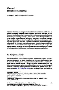
Fig. 1.
Mackey-Glass time series when Tau=17
[8]. In this paper, a forecasting method is proposed using an interval type-2 Mamdani model optimised using simulated annealing. The Mackey-Glass time series is a well known bench mark which will be used here as an application of forecasting. The rest of the paper starts by describing the data sets in section II followed by a review of fuzzy systems (section III) and simulated annealing (section IV). The methodology and the results of this paper are detailed in section V where the conclusion is drawn in section VI. II. M ACKEY-G LASS T IME S ERIES The Mackey-Glass Time Series is a chaotic time series proposed by Mackey and Glass [9]. It is obtained from this non-linear equation : dx(t) a ∗ x(t − τ ) = − b ∗ x(t) dt 1 + xn (t − τ ) Where a, b and n are constant real numbers and t is the current time where τ is the difference between the current time and the previous time t − τ . To obtain the simulated data, the equation can be discretised using the Fourth-Order Runge-Kutta method. In the case where τ > 17, it is known to exhibit chaos and has become one of the benchmark problems in soft computing [10, p.116]. III. T YPE -2 F UZZY S YSTEMS Type-1 fuzzy logic has been successful in many applications, However, the type-1 approach has problems when
WCE 2011
Proceedings of the World Congress on Engineering 2011 Vol II WCE 2011, July 6 - 8, 2011, London, U.K. faced with dynamical environments that have some kinds of uncertainties. These uncertainties exist in the majority of real world applications and can be a result of uncertainty in inputs, uncertainty in outputs, uncertainty that is related to the linguistic differences, uncertainty caused by the conditions change in the operation and uncertainty associated with the noisy data when training the FLC [11]. All these uncertainties translate into uncertainties about fuzzy sets membership functions [11]. Type-1 fuzzy Logic can not fully handle these uncertainties because type-1 fuzzy logic membership functions are totally precise which means that all kinds of uncertainties will disappear as soon as type-1 fuzzy set membership function has been used [12]. The existence of uncertainties in the majority of real world applications makes the use of type-1 fuzzy logic inappropriate in many cases especially with problems related to inefficiency of performance in fuzzy logic control [12]. Also, interval type2 fuzzy sets can be used to reduce computational expenses. Type-2 fuzzy systems have, potentially, many advantages over type-1 fuzzy systems including the ability to handle numerical and linguistic uncertainties, allowing for a smooth control surface and response and giving more freedom than type-1 fuzzy sets [12]. Since last decade, type-2 fuzzy logic is a growing research topic with much evidence of successful applications [13]. ˜ is characterized by A type-2 fuzzy set [11], denoted A, a type-2 membership function µA˜ (x, u) where x ∈ X and u ∈ Jx ⊆ [0, 1]. For example : A˜ = ((x, u), µA˜ (x, u)) | ∀x ∈ X, ∀u ∈ Jx ⊆ [0, 1]
Fig. 2.
•
•
where 0 ≤ µA˜ (x, u) ≤ 1. Set A˜ also can be expressed as: Z Z ˜ A= µA˜ (x, u)/(x, u), Jx ∈ [0, 1] R
x∈X
u∈Jx
where denotes union. When universe of discourse is discrete, Set A˜ is described as : X X A˜ = µA˜ (x, u)/(x, u), Jx ∈ [0, 1] x∈X u∈Jx
When all the secondary grades µA˜ (x, u) equal 1 then A˜ is an interval type-2 fuzzy set. Interval type-2 fuzzy sets are easier to compute with than general type-2 fuzzy sets. See Figure 2 for an example of an interval type-2 fuzzy set called “About 10“. The ease of computation and representation of interval type-2 fuzzy sets is the main reason for their wide usage in real world applications. Type-2 fuzzy logic systems are rule based systems that are similar to type-1 fuzzy logic systems in terms of the structure and components but type-2 FLS has an extra output process component which is called the type-reducer before defuzzification. The type-reducer reduces output type-2 fuzzy sets to type-1 fuzzy sets then the defuzzifier reduces it to a crisp output. The components of a type-2 fuzzy system are: •
Fuzzifier : Fuzzifier maps crisp inputs into type-2 fuzzy sets by evaluating the crisp inputs x = (x1, x2, . . . , xn) based on the antecedents part of the rules and assigns each
ISBN: 978-988-19251-4-5 ISSN: 2078-0958 (Print); ISSN: 2078-0966 (Online)
Interval type-2 fuzzy set “About 10“.
˜ crisp input to its type-2 fuzzy set A(x) with its membership grade in each type-2 fuzzy set. Rules: A fuzzy rule is a conditional statements in the form of IF-THEN where it contains two parts, the IF part called the antecedent part and the Then part called the consequent part. Inference Engine: Inference Engine maps input type-2 fuzzy sets into output type-2 fuzzy sets by applying the consequent part where this process of mapping from the antecedent part into the consequent part is interpreted as a type-2 fuzzy implication which needs computations of union and intersection of type-2 fuzzy sets and a composition of type-2 relations by using the extended sup-star composition for type-2 set relations. The inference engine in a Mamdani system maps the input fuzzy sets into the output fuzzy sets then the defuzzifier converts them to a crisp output. The rules in Mamdani model have fuzzy sets in both the antecedent part and the consequent part. For example, the ith rule in a Mamdani rule base can be described as follows: Ri : IF x1 is A˜i1 and x2 is A˜i2 ... and xp is A˜ip THEN y is B˜i
•
Output Processor: There are two stages in the output process: – Type-Reducer: Type-reducer reduces type-2 fuzzy sets that have been produced by the inference engine to type1 fuzzy sets by performing a centroid calculation [10].T – Defuzzifier: Defuzzifier maps the reduced output type-1 fuzzy sets that have been reduced by type-reducer into crisp values exactly as the case of defuzzification in type-1 fuzzy logic systems.
WCE 2011
Proceedings of the World Congress on Engineering 2011 Vol II WCE 2011, July 6 - 8, 2011, London, U.K. IV. S IMULATED A NNEALING A LGORITHM The concept of annealing in the optimisation field was introduced by Kirkpatrick et al in 1982 [14]. Simulated annealing uses the Metropolis algorithm to imitate metal annealing in metallurgy where heating and controlled cooling of materials is used to reshape metals by increasing the temperature to the maximum values until the solids almost melted then decreasing the temperature carefully until the particles are arranged and the system energy becomes minimal. Simulated annealing is a powerful randomised local search algorithm that has shown great success in finding optimal or nearly optimal solutions of combinatorial problems [15]. SA is particularly useful in high dimensionality problems as it scales so well with the increase of variable numbers which allows SA to be a good candidate for fuzzy systems optimisation [16]. Many comparative studies for solving problems such as job shop scheduling and travelling sales man suggest that SA can outperform most other local search algorithms in terms of effectiveness [15]. In general, SA can find good solutions for a wide range of problems but normally with the cost of high running times [15]. We now define the simulated annealing algorithm. Let s be the current state and N (s) be a neighbourhood of s that includes alternative states. By selecting one state s′ ∈ N (s) and computing the difference between the current state cost and the selected state energy as D = f (s′ ) − f (s), s′ is chosen as the current state based on Metropolis criterion in two cases: • If D < 0 means the new state has a smaller cost, then s′ is chosen as the current state as downhills always accepted. ′ • If D > 0 and the probability of accepting s is larger than a random value Rnd such that e−D/T > Rnd then s′ is chosen as the current state where T is a control parameter known as Temperature which is gradually decreased during the search process making the algorithm more greedy as the probability of accepting uphill moves decreasing over time. Rnd is a randomly generated number where 0 < Rnd < 1. Accepting uphill moves is important for the algorithm to avoid being stuck in a local minima. In the last case where D > 0 and the probability is lower than the random value e−d/T