Tunnel-MILP: Path Planning with Sequential Convex ... - CiteSeerX

Tunnel-MILP: Path Planning with Sequential Convex Polytopes∗ Michael P. Vitus†, Vijay Pradeep‡, Gabriel M. Hoffmann§, Steven L. Waslander¶ and Claire J. Tomlin k This paper focuses on optimal path planning for vehicles in known environments. Previous work has presented mixed integer linear programming (MILP) formulations, which suffer from scalability issues as the number of obstacles, and hence the number of integer variables, increases. In order to address MILP scalability, a novel three-stage algorithm is presented which first computes a desirable path through the environment without considering dynamics, then generates a sequence of convex polytopes containing the desired path, and finally poses a MILP to identify a suitable dynamically feasible path. The sequence of polytopes form a safe tunnel through the environment, and integer decision variables are restricted to deciding when to enter and exit each region of the tunnel. Simulation results for this approach are presented and reveal a significant increase in the size and complexity of the environment that can be solved.

I.

Introduction

Increased autonomy in the operation of uninhabited aerial and ground systems (UASs,UGSs) continues to be identified as a pressing concern for the adoption and commercialization of these systems in everyday life. Despite recent successes such as the NASA Mars Rovers1 and the DARPA Grand Challenges,2, 3 many barriers remain for the deployment of autonomous vehicles in both military and civilian applications. In particular, the automation of the task of vehicle motion planning remains challenging as the size, complexity and dimension of the environment to be planned in increases. To this end, this work develops a novel multi-stage path planning algorithm that seeks near optimal solutions that satisfy linear vehicle dynamic constraints. The main motivation for this comes from the desire to enable increased autonomy on the Stanford Testbed of Autonomous Rotorcraft for Multi-Agent Control (STARMAC), currently under development at Stanford.4, 5 As the testbed vehicles are designed as mobile sensor networks for applications such as cooperative search in unknown environments, the ability to quickly and reliably navigate through cluttered surroundings is critical to enabling higher levels of automation and multi-vehicle coordination. With limited payload capacity, on-board computational resources are at a premium, resulting in the need for fast on-board path planning algorithms. Solving an obstacle avoidance problem for a linear system with constraints on the states can be posed as a mixed integer linear program (MILP). In this approach,6 obstacles are included as sets of OR constraints, where at least one of the constraints defining the edges of each obstacle must be satisfied. The resulting ∗ This research was supported by the ONR under the CoMotion MURI grant N00014-02-1-0720 and the DURIP grant N00014-05-1-0443, as well as by NASA grant NNAO5CS67G. † Ph.D. Candidate, Department of Aeronautics and Astronautics, Stanford University. AIAA Student Member. [email protected] ‡ Masters Student, Department of Mechanical Engineering, Stanford University. [email protected] § Ph.D. Candidate, Department of Aeronautics and Astronautics, Stanford University. AIAA Student Member. [email protected] ¶ Post-Doctoral Scholar, Department of Aeronautics and Astronautics, Stanford University. AIAA Member. [email protected] k Professor, Department of Electrical Engineering and Computer Sciences, University of California at Berkeley. Research Professor, Department of Aeronautics and Astronautics; Director, Hybrid Systems Laboratory, Stanford University. AIAA Member. [email protected]

1 of 13 American Institute of Aeronautics and Astronautics

MILP does not scale very well with the number of obstacles in the environment. Since each obstacle edge requires a set of binary variables for every timestep under consideration, the number of binary variables scales linearly in the number of obstacle edges. It is well known that MILP is NP-hard in the number of binary variables used in the problem formulation,7, 8 and so computational requirements grow exponentially as the number of binary variables needed to model the problem increases. The result is an algorithm that can manage at most a limited number of obstacles in a reasonable time for applications such as those envisaged for STARMAC. Instead, this work proposes to break down the task of determining a dynamically feasible trajectory through an obstacled environment into a three step algorithm. First, a desirable path is determined without any consideration of vehicle dynamics. This can be done with either a visibility graph approach to finding the shortest path,9, 10 or by gradient descent of a fast-marching potential.11, 12 Next, a tunnel is formed through the environment as a sequence of convex polytopes through which the vehicle must travel. Finally, a dynamically feasible trajectory is generated using a MILP formulation that restricts the vehicle’s path to stay within the pre-defined tunnel. The Tunnel-MILP method relies on the following insight: requiring the state to remain inside a convex polytope requires no binary variables, whereas requiring the state to remain outside a convex polytope requires one for each edge. By first determining a path ignoring the vehicle’s dynamics, then identifying the sequence of convex regions through which to travel, the resulting MILP needs only determine at which timestep to make the transition from one polytope to the next. Care in formulating the MILP has proven useful in other aerospace applications as well.13, 14 In all these cases, the result is a problem formulation with fewer binary decision variables, and therefore, with the potential for slower growth in computation time. Other attempts have been made to address the issue of problem size in MILP formulations of the obstacle avoidance problem. Bellingham, Richards, and How15 developed a receding horizon MILP controller to plan short trajectories around nearby obstacles. Earl and D’Andrea16 have proposed an iterative method for including obstacles as they are detected to interfere with the current best route. Their algorithm seeks to ensure continuous time obstacle avoidance, and to find minimum time solutions through binary search with a continuous end time. As the density of obstacles and the complexity of the environment increases, the number of MILP instances can grow quickly, resulting in slow performance of the algorithm. For problems with a very large number of constraints, there do exist randomized methods, such a probabilistic roadmaps (PRM).17 Computation time for PRMs scales with the expansiveness of the space, as opposed to the number of obstacles or binary constraints. This makes PRMs attractive for large problems; however, optimality is not explicitly considered in the problem formulation, often resulting in windy or sinuous paths if vehicle dynamics are incorporated. The paper proceeds as follows. Section II presents a standard MILP formulation of the path planning problem based on work by Richards et al.6 Then, each of the three stages of the Tunnel-MILP algorithm are described in detail in Section III. In Section IV, an analysis of the computational complexity and solution optimality are presented. A breakdown of the computation times for the Tunnel-MILP algorithm and comparison with previous methods are presented in Section V. Finally, Section VI includes a brief discussion of directions of future improvements.

II.

Problem Formulation

The environment under consideration is assumed to be a bounded convex polytope in 2-D. Let N E be E E the number of edges of the polytope, F E ∈ RN ×2 define the outward normals to each edge, and GE ∈ RN be the offset. Then the environment E = {x ∈ R2 |F E x − GE ≤ 0} ⊂ R2 is defined to be the interior of the polytope. Similarly, obstacles can be defined that lie inside the environment. Let N O be the number of obstacles, and for each obstacle i, let NiO be the number of edges. Each obstacle Oi ∈ O can then be defined analogously O NiO to the environment with components FiO ∈ RNi ×2 and GO . i ∈R The obstacle avoidance problem is posed over a finite time horizon Tmax ∈ R with T timesteps of fixed length δt ∈ R. The vehicle navigating through this environment is modeled with standard linear point mass dynamics, p(t + 1) = p(t) + v(t)δt + u(t)δt2 /2 (1) v(t + 1) = v(t) + u(t)δt

2 of 13 American Institute of Aeronautics and Astronautics

where the position p(t) = (x(t), y(t)) ∈ E at each timestep, t ∈ {1, . . . , T }, is constrained to lie in the environment, and the velocity v(t) ∈ R2 and acceleration control inputs u ∈ R2 are bounded. F E p(t) − GE ≤ 0 , ∀t ∈ {1, . . . , T } ∀t ∈ {1, . . . , T } v ≤ v(t) ≤ v¯ , u ≤ u(t) ≤ u ¯, ∀t ∈ {1, . . . , T }

(2)

Furthermore, the vehicle is assumed to start at some initial position and velocity and to have a known final goal at unknown final time tf . p(0) = p0 ,

v(0) = v0 ,

p(tf ) = pf

(3)

In formulating the obstacle avoidance problem considered in this work, both minimum time and minimum control input models are included, and combined linearly to define a family of possible optimization programs. The cost function used is as follows, J(u, tf ) = γtf + (1 − γ)

T X

(|ux (t)| + |uy (t)|)

(4)

t=1

where γ ∈ [0, 1] defines the tradeoff between control authority and time of completion of the trajectory. In order to encode both the avoidance of obstacle regions and the free end-time constraint in a MILP formulation, binary decision variables are added to the problem formulation. Obstacle avoidance can be ensured by requiring that at least one edge-defining constraint is not violated. Following previous work,6 a binary decision variable, b(t, i, j) ∈ {0, 1}, is defined for each edge j ∈ {1, . . . , NiO } of each obstacle Oi ∈ O at each timestep t, which decides if the associated constraint is active. By requiring at least one edge constraint to be active for every obstacle at each timestep, all feasible paths will necessarily avoid the obstacles. O Fi,j p(t) − GO ≥ 0 i,j O N i P b(t, i, j) ≥ 1

if b(t, i, j) = 1 (5)

j=1

The variable final time is also encoded by adding an additional binary decision variable f (t) at each timestep, which relaxes the dynamic constraints once the final position is achieved, essentially nullifying the problem once the goal is achieved. f (t + 1) ≥ f (t) f (1) = 0 , f (T ) = 1 T P (6) tf ≥ (1 − f (t)) t=1

p(t) = pf

if f (t) = 1

The Standard MILP obstacle avoidance problem is now stated.6 Standard MILP minimize subject to

J(u, tf ) (1) if f (t) = 0 (2), (3) (5), (6)

(P2.1)

Optimal solutions to the standard MILP program can be found efficiently by encoding the problem in the AMPL18 programming language and using a commercial MILP solver such as CPLEX.19 However, as the number of binary variables grows linearly in the length of the time horizon and in the number of obstacles, the computational burden can rapidly exceed reasonable times for autonomous applications. As a result, there exists a need for alternative solution methodologies to tackle large optimal path planning problems, such as the Tunnel-MILP algorithm outlined in the following section. 3 of 13 American Institute of Aeronautics and Astronautics

Start

Goal

(a)

(b)

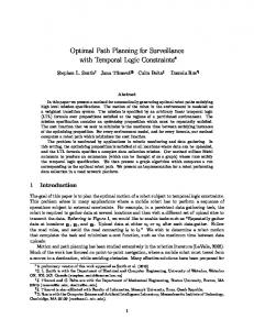
Figure 1. (a) Visibility graph, with shortest path highlighted (b) Fast marching potential function with steepest descent path highlighted.

III.

The Tunnel-MILP Algorithm

The Tunnel-MILP algorithm is composed of three main steps. First, a shortest path to the goal is generated while ignoring the vehicle’s dynamics constraints. Next, this path is combined with a convex decomposition of the free space to generate a sequence of convex polytopes from the start to the goal. Finally, this tunnel of polytopes is used to constrain the MILP to find the optimal, dynamically feasible path to the goal. A.

Pre-Path Generation

The first step in Tunnel-MILP is to generate the pre-path. In general, the optimal dynamically feasible path is close to the shortest path while ignoring dynamics. Therefore, it seems reasonable to use the shortest path, or something close to the shortest path, as a pre-path to generate the convex polytope sequence for the MILP. Two methods for pre-path generation are a visibility graph and fast marching. 1.

A-Star and Visibility Graph

For a 2D space, a visibility graph stores the connectivity between a start node, end node, and obstacle vertices. Any two vertices are considered connected if there exists a straight-line path between them that does not pass through any obstacles.10 In the most basic implementation, every possible edge (generated from every possible set of 2 nodes) is checked for collision against every obstacle in the space, taking O(n3 ) time. However, there are more advanced methods that generate the graph in O(n2 ) time.9 Once the visibility graph is generated, an A-Star graph search can very efficiently find the shortest distance path from the start to goal node, as shown in Figure 1(a). 2.

Fast Marching

Fast marching differs from other path generation methods in that nodes along the path are not restricted to obstacle vertices. Originally developed by Osher12 and Sethian,11 fast marching is a level-set method that generates a discretized cost-to-go function for the entire environment by propagating a wavefront starting

4 of 13 American Institute of Aeronautics and Astronautics

Fast-Marching Solution

Start

Goal

Visibility Graph Solution

Figure 2. Fast-Marching is biased towards open spaces.

from the goal location. It can be thought of as a smart dynamic program that interpolates between grid cells to find an approximate solution to the following partial differential equation, known as the Eikonal equation. |∇u(x)| = F (x)

(7)

For the shortest path formulation, x ∈ R2 is the vehicle position, u(x) is the navigation (or cost-to-go) function, and F (x) is the obstacle penalty function. Fast marching is initialized with u(pf ) = 0, and the cells neighboring the final position, pf , form the initial propagation wavefront. The algorithm freezes the lowest cost cell on the wavefront, computes costs for its unfrozen neighbors, and then adds them to the wavefront. This causes the wavefront to grow from the goal, with speed inversely proportional to F (x). By choosing to always update the lowest cost cell on the wavefront, the algorithm never has to revisit cells, resulting in fast computation times for the entire workspace. Given that the fast marching propagation approximates a dynamic program through the workspace, its navigation function does not have any local minima. This is a significant advantage over other field based schemes, such as the potential field method,10 since gradient descent from the start position always generates a path to the goal, as demonstrated in Figure 1(b). One very simple penalty function is F (x) = 1 + 1/d(x) (8) where d(x) is the distance to the nearest obstacle. Hence, there is a high cost near obstacles, and a cost of 1 when far from obstacles. Because of the high penalty when close to obstacles, the shortest path is biased away from obstacles. This helps mimic the acceleration constraints of the vehicle, since the vehicle generally has to slow down when performing tight maneuvers around obstacles, as demonstrated in Figure 2. B.

Free Space Decomposition

After computing the pre-path, a sequence of convex polytopes that encloses the pre-path is found. The space is first decomposed into convex polytopes, either through trapezoidal decomposition or Delaunay triangulation, and then the polytopes that pass through the pre-path are added to the tunnel. 1.

Trapezoidal Decomposition

Trapezoidal decomposition, also known as the line-sweep method, is a decomposition method first proposed in 1987.20 The method proceeds by sweeping a vertical line through the workspace from left to right. As each vertex is encountered, a new set of polytopes is generated by inserting a vertical slice. The decomposition runs at O(n log n), but it’s important to realize that, in general, the computed trapezoidal polytopes cannot be combined into larger convex regions (see Figure 3(a). This results in a relatively large number of polygonal regions, and thus a large number of binary variables for the MILP.

5 of 13 American Institute of Aeronautics and Astronautics

1

4 2

5 6

3

3 1

1

2

(a)

3

(b)

2

(c)

Figure 3. (a) Trapezoid Decomposition and resulting polytope tunnel (b) Delaunay triangulation of free space (c) Resulting tunnel with merged convex polytopes

2.

Delaunay Triangulation

In a Delaunay triangulation, the circumscribed circle of any triangle in the mesh will not contain any nodes.21 This generally results in the triangulation avoiding highly eccentric triangles, thus helping to create a much more even mesh. Any triangles that are completely contained in obstacles can be removed from the mesh, and triangles that pass through obstacles can be cut in half so that the part of the triangle in the obstacles can be removed. As an alternative to heuristically removing regions that are in conflict with obstacles, it is also possible to perform constrained Delaunay triangulation to generate the mesh in the presence of obstacles in O(n log n) time,22 but this is an area of future investigation. Superimposing the pre-path onto the Delaunay triangulation generates the sequence of polytopes (in this case triangles) for the Tunnel-MILP, but the number of included triangles can become quite large, even in somewhat simple environments, such as in Figure 3(b). However, in many cases, triangles along the tunnel can be merged into larger convex polytopes in a sequential manner. That is, the first triangle is merged with as many downstream triangles as possible, until the polytope becomes non-convex. The offending triangle is then used to start a new polytope, and the process is repeated until the goal is reached, as in Figure 3(c). This method significantly reduces the number of polytopes needed to enclose the pre-path, but it does not necessarily use the fewest possible polytopes nor cover the largest possible area. Optimal convex decompositions23 could be used to generate a better polytope sequence if necessary, but in practice the benefits of the more complex method are limited. C.

MILP with Sequential Convex Polytopes

Each convex region of the tunnel, Ri , is defined as a conjunction of linear constraints similar to the definition of the environment. N R is the total number of regions, NiR is the number of edges in the ith region, R NiR FiR ∈ RNi ×2 define the outward normals to each edge and GR is the offset.24 For the sequence of i ∈ R convex polytopes, the vehicle is constrained to remain in at least one region at all times, t, as follows, _ FiR p (t) − GR (9) i ≤ 0 ∀ t ∈ {1, . . . , T } i∈{1,...,N R }

The OR-constraints are once again incorporated into the MILP formulation by introducing binary variables β(t, i), where t ∈ {1, . . . , T } and i ∈ {1, . . . , N R }. ( 1 if the vehicle has arrived at region i by timestep t (10) β(t, i) = 0 otherwise The binary variable β(t, i) is 1 for all timesteps after which the vehicle first arrives in the specific region, i.

6 of 13 American Institute of Aeronautics and Astronautics

Boundary conditions on the binary decision variable are set to require starting in the first region and ending in the final region by timestep T . β(t − 1, i) ≤ β(t, i) ∀t ∈ {2, . . . , T }, i ∈ {1, . . . , N R } β(t, 1) = 1 ∀t ∈ {1, . . . , T } β(T, i) = 1 ∀i ∈ {1, . . . , N R }

(11)

Since the regions are sequenced together to form a tunnel through the environment, the following constraint enforces the sequential ordering of the polytopes β(t, i + 1) ≤ β(t, i) ∀t ∈ {1, . . . , T }, i ∈ {1, . . . , N R − 1}

(12)

which states that the regions must be traversed in sequential order. From the binary constraints, the active region at timestep, t, can be found by taking the following difference of the binary variables, ρ(t, i) = β(t, i) − β(t, i + 1) ρ(t, N R ) = β(t, N R )

∀t ∈ {1, . . . , T }, i ∈ {1, . . . , N R − 1} ∀t ∈ {1, . . . , T }

(13)

where ρ(t, i) indicates whether region i is the active region at time t. A subtlety of the constraints in Equations (11) and (12) is that it allows regions to be skipped; this can be verified by observing that if β(t − 1, i) = β(t − 1, i + 1) = 0 and β(t, i) = β(t, i + 1) = 1, then Equations (11) and (12) are still satisfied, implying that no timestep exists for which the vehicle position lies within region i. A method used to invalidate constraints when inactive is called the big-M formulation;25 it uses a large, positive constant, M , to invalidate the constraint when a binary variable indicates it is inactive. Using Equations (12) and (13) and the big-M formulation to invalidate the constraints when the vehicle is not inside the region, the vehicle can be constrained to sequentially go through the polytopes. FiR p(t) − GR i ≤ M (1 − ρ(t, i))

∀t ∈ {1, . . . , T }, i ∈ {1, . . . , N R }

(14)

Finally, the overall MILP optimization problem with sequential convex polytopes formulation can be stated. Sequential convex polytope program minimize subject to

J(u, tf ) (1) if f (t) = 0 (2), (3), (6) (11), (12), (14)

(P3.1)

The following section provides a brief analysis of the optimality of the solution for the Tunnel-MILP algorithm as well as the computational complexity.

IV.

Algorithmic Analysis

By decomposing the obstacle avoidance problem into three stages, the Tunnel-MILP algorithm seeks to gain performance improvements over the standard MILP methodology without sacrificing too much in the way of optimality of the solution. Necessarily, the selection of a specific tunnel of polygons through which to travel restricts the set of dynamically feasible solutions that can be achieved and may eliminate the true optimal solution as part of the first two stages of the algorithm. It is therefore no longer possible to guarantee global optimality of the solution generated by the Tunnel-MILP algorithm. However, the path found in the third phase of the algorithm is the optimal path that can be found within the sequence of polygons selected. The likelihood of significant differences between the global optimal solution and the Tunnel-MILP solution depends directly on the ability of the vehicle to navigate sharp corners along the desired path generated in the algorithms second stage. If, for example, the acceleration bounds are tight and the requirement to satisfy vehicle dynamics becomes quite restrictive, then a long arching route around a set of obstacles may proceed much more quickly than a slower route through tight passages in the environment. This issue is quantified 7 of 13 American Institute of Aeronautics and Astronautics

in Section V below, where it can be noted that for most solutions found to differ from the optimal, both final time differences and control cost differences were small. This issue is aggravated by the fact that the visibility graph often returns a path with sharp corners, and does not in any way take into consideration the size of the passageway through which the vehicle must travel. It is for this reason that the fast-marching method is also presented in Section A, as the speed of the wave propagation is dependent on the proximity to obstacles, and would result in higher cost potentials in narrow passages. As a result, the gradient descent pre-path tends to avoid such passages (see Figure 2). The benefit, then, of employing the three stage Tunnel-MILP algorithm lies in the reduced complexity of the resulting MILP formulation. The number of binary variables related to obstacles in the standard PN O MILP formulation is T ( i=1 NiO ) whereas for the Tunnel-MILP it is T N R . Since the number of tunnel regions tends to grow more slowly than the number of facets of obstacles, it is likely that as the problem size increases, the Tunnel-MILP formulation will return solutions more quickly. It should be noted that the first two stages of the algorithm can be solved in negligible time relative to the MILP for the problem sizes under consideration.

V.

Simulation Results

The standard and Tunnel-MILP algorithms were tested on 600 randomly generated environments with a number of obstacles from 3 to 9 and 10 randomly generated environments for 20 obstacles. The initial state was p(0) = (0.1, 0.1) m and v(0) = (0, 0) m/s with a final position of p(tf ) = (11.5, 8.5) m. The velocity constraints are −2 m/s ≤ v(t) ≤ 2 m/s and the input constraints are −0.5 m/s2 ≤ u(t) ≤ 0.5 m/s2 . The bounds on the environment are 0 m ≤ x(t) ≤ 13 m and 0 m ≤ y(t) ≤ 10 m. The discretization of the continuous dynamics used was δt = 0.1 seconds. The obstacles considered are rectangles with randomly chosen position and edge lengths, but were not allowed to lie outside the environment or overlap other obstacles. Table 1 summarizes the percentage of area covered by the obstacles in the environment, which corresponds to how dense the obstacles were in the test environments. A time limit of 600 seconds was placed on both algorithms for 3 to 9 obstacles, and a time limit of 1200 seconds was placed on the 20 obstacle case. To solve both MILP programs, CPLEX19 with an AMPL18 interface was used on dual 3GHz Xeon processors with 8 GB of RAM. Although these computation times exceed the allowable computation timeframes for most applications, the comparison remains a good indication of the scalability of the algorithm, as computation power continues to improve in the future. Table 1. Percentage of Obstacle Area

# Obstacles 3 4 5 6 7 8 9 20

% Area 24.68 30.72 34.13 36.29 34.28 33.27 33.91 19.62

Figure 4 shows the average computation time for the Tunnel-MILP algorithm using either trapezoidal or Delaunay decomposition and the standard MILP algorithm for all cases in which either algorithm found a solution within the time limit. As shown in the figure, the Tunnel-MILP algorithm outperforms the standard MILP algorithm in terms of computation time, and suggests that as the number or density of obstacles increases the Tunnel-MILP algorithm will grow at a slower rate computationally than the standard MILP algorithm. For the 20 obstacle scenario, the standard MILP computation time is 271.7 seconds whereas the trapezoidal and Delaunay decomposition for Tunnel-MILP is 42.1 and 50.6 seconds, respectively, which corresponds to approximately a factor of six speedup. The computation time for the Tunnel-MILP algorithm to calculate the optimal path through the tunnel varies based upon which decompositional method is

8 of 13 American Institute of Aeronautics and Astronautics

employed. Even though Delaunay decomposition produces fewer convex regions than trapezoidal decomposition, it results in a longer computation time for the Tunnel-MILP algorithm. Table 2 shows the average timestep increase and input cost difference between the Tunnel and standard MILP algorithms when the standard MILP algorithm finds a solution. As shown in the table, there is only a slight increase in the number of timesteps for the Tunnel-MILP algorithm above the optimal final time; the input cost difference is also negligible between the two algorithms. Both of these factors suggest that the significant decrease in the computation time for the Tunnel-MILP algorithm offsets the slight increase in the cost function for the Tunnel-MILP algorithm over the standard MILP method. Table 2. Comparison of the percent average timestep and input cost increase between the standard and Tunnel-MILP, with trapezoidal decomposition, solutions for problems that they both were able to solve.

# Obstacles

% Avg. Timestep Increase

% Avg. Input Cost Increase

7.78 3.69 2.01 1.77 2.55 1.69 1.94 0.73

14.94 13.96 8.06 3.69 9.23 6.61 4.94 3.82

3 4 5 6 7 8 9 20

Comparison of Computation Time

Average Computation Time (sec)

250 Standard MILP Trapezoidal−Tunnel Delaunay−Tunnel

200

150

100

50

0

3

4

5

6

7

8

9

Number of Obstacles

Figure 4. Comparison of Computational Time of the Tunnel and Standard MILP

Figure 5 shows the fraction of instances solved versus computation time required for both algorithms. As shown in the figures, the Tunnel-MILP algorithm is less computationally intensive than the standard MILP algorithm in all cases considered. After 200 seconds, the Tunnel-MILP algorithm has solved 75% of the instances for all number of obstacles. In contrast, the standard MILP algorithm solves 75% of the instances for only the 3, 4 and 5 obstacle cases, and for the environments with 6, 7, 8 and 9 obstacles it is unable to solve more than 75% of the instances before the time limit elapses. Figure 6 shows a comparison of the trapezoidal decomposition and the optimal paths from the standard and Tunnel-MILP algorithms on the 3 and 5 obstacle environments. For Figures 6 (a), (b) and (d), the standard MILP algorithm trajectory traverses a big arc to the goal, but for the Tunnel-MILP algorithm the pre-path has biased the trajectory through a much more varying path which is higher in the total input cost. For Figure 6 (c), since the pre-path chooses a tunnel along the optimal path, the tunnel and standard MILP algorithms produce the exact same trajectory.

9 of 13 American Institute of Aeronautics and Astronautics

Standard MILP 1

0.9

0.9

0.8

0.8

Fraction of instances solved

Fraction of instances solved

Tunnel MILP 1

0.7 0.6 0.5 0.4 3 obstacles 4 obstacles 5 obstacles 6 obstacles 7 obstacles 8 obstacles 9 Obstacles

0.3 0.2 0.1 0

0

100

200

300

400

0.7 0.6 0.5 0.4 3 obstacles 4 obstacles 5 obstacles 6 obstacles 7 obstacles 8 obstacles 9 Obstacles

0.3 0.2 0.1

500

0

0

100

Computation Time (sec)

200

300

400

500

Computation Time (sec)

(a)

(b)

Figure 5. Percentage complete versus computational time (a) Tunnel-MILP with trapezoidal decomposition (b) Standard MILP

A comparison of the paths produced by both algorithms on a 20 obstacle environment is shown in Figure 7. The computation time for the Tunnel-MILP algorithm was 95.1 seconds and the standard MILP algorithm was 446.3 seconds, which is a factor of 4.7 speedup. The Tunnel-MILP algorithm’s solution reached the goal position 3 timesteps after the standard MILP’s solution. The input cost for the Tunnel-MILP algorithm is 63.9 and 55.8 for the standard MILP algorithm. As shown in the figure, the environment provides a choice in the middle of the trajectory to traverse to the left or right of the obstacles. The pre-path biases the trajectory for the Tunnel-MILP algorithm to the right but reduces the number of choices for the algorithm. Although the pre-path biased the algorithm in the non-optimal direction, the solution was only penalized a small amount but realized a significant decrease in the computation time because of it.

VI.

Conclusions and Future Work

The Tunnel-MILP algorithm presented in this work provides significant performance improvements over previous methods for large scale obstacle avoidance problems. While some problem instances resulted in deviations from the globally optimal trajectory, the accompanying changes in final time of arrival and control cost were often not very large. By decomposing the path planning process with dynamic constraints into a three stage optimization, it was possible to increase the size of planning problems that can be addressed in practice for applications where vehicle dynamics are an important consideration. Some extensions to the Tunnel-MILP that may significantly improve performance have been identified as areas for future investigation. The ability to shrink the trapezoids in areas where the trajectory is very unlikely to traverse and merge trapezoids in open areas may lead to reductions in the number of binary variables associated with the problem. By performing this merging process, the optimization problem may gain a major speedup in computation time. Another area of interest is to analyze the characteristics of the resulting tunnel to determine how different decompositions affect the computational time. Furthermore, the Tunnel-MILP algorithm will be incorporated as part of the onboard computational processing for the STARMAC platform of vehicles. Both the platform and the algorithm are certain to benefit from the real-world experience that will result.

References 1 Helmick, D., Angelova, A., Livianu, M., and Matthies, L., “Terrain Adaptive Navigation for Mars Rovers,” Aerospace Conference, 2007 IEEE , 2007, pp. 1–11. 2 Thrun, S., Montemerlo, M., Dahlkamp, H., Stavens, D., Aron, A., Diebel, J., Fong, P., Gale, J., Halpenny, M., Hoffmann, G., Lau, K., Oakley, C., Palatucci, M., Pratt, V., Stang, P., Strohband, S., Dupont, C., Jendrossek, L.-E., Koelen, C., Markey, C., Rummel, C., van Niekerk, J., Jensen, E., Alessandrini, P., Bradski, G., Davies, B., Ettinger, S., Kaehler, A., Nefian, A.,

10 of 13 American Institute of Aeronautics and Astronautics

Example Environment

Example Environment

10

10 5

9

6

9

8

8

7

7 1

7

6 5

4

5 1

4

4

3

3 2

2

9

6

3

4

10 8 7

5

2

6 2

1

1 3

0

0 0

2

4

6

8

10

12

0

2

4

6

8

10

12

10

12

Standard MILP Tunnel MILP

Standard MILP Tunnel MILP

(a)

(b)

Example Environment

Example Environment

10

10 9

9

6

10

9 5

8

8

7 5 6

6

7

8

7

11

6

4

5 1

5 1

4

4 4

3

2

3

3

2

2

1

1

0

2

3

0 0

2

4

6

8

10

12

0

2

4

6

8

Standard MILP Tunnel MILP

Standard MILP Tunnel MILP

(c)

(d)

Figure 6. Comparison between the path generated by the Tunnel-MILP versus Standard MILP. The obstacles are red, the underlying sequence of convex polytopes are numbered, the standard MILP path is red and the tunnel MILP path is blue.

11 of 13 American Institute of Aeronautics and Astronautics

Example Environment 10 9 8 7 6 5 4 3 2 1 0

0

2

4

6 8 Standard MILP Tunnel−MILP

10

12

Figure 7. Comparison between the path generated by the Tunnel-MILP versus Standard MILP for a 20 obstacle case. The trapezoidal decomposition produced 35 polytopes.

and Mahoney, P., “Stanley: The robot that won the DARPA Grand Challenge,” Journal of Field Robotics, Vol. 23, No. 9, September 2006, pp. 661–692. 3 Thrun, S., “Why we compete in DARPA’s Urban Challenge autonomous robot race,” Commun. ACM , Vol. 50, No. 10, 2007, pp. 29–31. 4 Waslander, S. L., Hoffmann, G. M., Jang, J. S., and Tomlin, C. J., “Multi-Agent Quadrotor Testbed Control Design: Integral Sliding Mode vs. Reinforcement Learning,” In Proceedings of the IEEE/RSJ International Conference on Intelligent Robotics and Systems 2005 , Edmonton, Alberta, August 2005, pp. 468–473. 5 Hoffmann, G., Huang, H., Waslander, S., and Tomlin, C. J., “Quadrotor Helicopter Flight Dynamics and Control: Theory and Experiment,” AIAA Guidance, Navigation and Control Conference and Exhibit, August 2007. 6 Richards, A., Kuwata, Y., and How, J., “Experimental Demonstrations of Real-time MILP Control,” Proceeding of the AIAA Guidance, Navigation, and Control Conference, August 2003. 7 Garey, M. R. and Johnson, D. S., Computers And Intractability: A guide to the Theory of NP-Completeness, W. H. Freeman and Co., New York, NY, USA, 1979. 8 Papadimitriou, C. H. and Steiglitz, K., Combinatorial Optimization: Algorithms and Complexity, Dover Publications, Inc., Mineola, NY, USA, 1998. 9 Asand, T., Asano, T., Guibas, L., Hershberger, J., and Imai, H., “Visibility of Disjoint Polygons,” Algorithmica, Vol. 1, 1986, pp. 49–63. 10 Latombe, J.-C., Robot Motion Planning, Kluwer Academic Publishers, Boston, MA, USA, 1991. 11 Kimmel, R. and Sethian, J., “Computing geodesic paths on manifolds,” Proceedings of National Academy of Sciences, Vol. 95, 1998, pp. 8431–8435. 12 Osher, S. and Fedkiw, R., Level Set Methods and Dynamic Implicit Surfaces, Springer-Verlag, New York, NY, USA, 2002. 13 Bertsimas, D. and Patterson, S. S., “The Air Traffice Flow Management Problem with Enroute Capacities,” Operations Research, Vol. 46, No. 3, 1998, pp. 406–422. 14 Bayen, A., Computational Control of Networks of Dynamical Systems: Application to the National Airspace System, Ph.D. thesis, Stanford University, December 2003. 15 Bellingham, J., Richards, A., and How, J., “Receding Horizon Control of Autonomous Aerial Vehicles,” Proceedings of the American Control Conference, Vol. 5, 2002, pp. 3741–3746. 16 Earl, Matthew. G. D’Andrea, R., “Iterative MILP methods for vehicle-control problems,” Robotics, IEEE Transactions on [see also Robotics and Automation, IEEE Transactions on] , Vol. 21, No. 6, 2005, pp. 1158–1167. 17 Kavraki, L. E., Svestka, P., Latombe, J.-C., and Overmars, M. H., “Probabilistic Roadmaps for Path Planning in HighDimensional Configuration Spaces,” Robotics, IEEE Transactions on [see also Robotics and Automation, IEEE Transactions on] , Vol. 12, No. 4, 1996, pp. 566–580. 18 AMPL Website, http://www.ampl.com, visited January 2008.

12 of 13 American Institute of Aeronautics and Astronautics

19 ILOG

CPLEX Website, http://www.ilog.com/products/cplex , visited January 2008. B., Advances in Robotics, Vol.1: Algorithmic and Geometric Aspects of Robotics, chap. Approximation and Decomposition of Shapes, Lawrence Erlbaum Associates, 1987, pp. 145–185. 21 Lee, D. and Schachter, B., “Two Algorithms for Constructing a Delaunay Triangulation,” International Journal of Computer and Information Sciences, Vol. 9, No. 3, 1980, pp. 219–242. 22 Chew, L. P., “Constrained Delaunay triangulations,” SCG ’87: Proceedings of the third annual symposium on Computational geometry, ACM, New York, NY, USA, 1987, pp. 215–222. 23 Chazelle, B. and Dobkin, D., Computational Geometry, chap. Optimal Convex Decompositions, Elsevier Science Publishers B.V., 1985, pp. 63–133. 24 Blackmore, L., “A Probabilistic Particle Control Approach to Optimal, Robust Predictive Control,” In the Proceeding of the AIAA Guidance, Navigation, and Control Conference, August 2006. 25 Bemporad, A. and Morari, M., “Control of systems integrating logic, dynamics, and constraints,” Automatica, Vol. 35, No. 3, 1999, pp. 407–427. 20 Chazelle,

13 of 13 American Institute of Aeronautics and Astronautics