Turbulence and Gravity Waves within an Upper-Level Front

NOVEMBER 2005

KOCH ET AL.

3885

Turbulence and Gravity Waves within an Upper-Level Front STEVEN E. KOCH,* BRIAN D. JAMISON,*,⫹ CHUNGU LU,*,⫹ TRACY L. SMITH,*,⫹ EDWARD I. TOLLERUD,* CECILIA GIRZ,* NING WANG,*,⫹ TODD P. LANE,# MELVYN A. SHAPIRO,@ DAVID D. PARRISH,& AND OWEN R. COOPER&,** * NOAA/Research–Forecast Systems Laboratory, Boulder, Colorado ⫹ Cooperative Institute for Research in the Atmosphere, Colorado State University, Fort Collins, Colorado # National Center for Atmospheric Research, Boulder, Colorado @ NOAA/Office of Weather and Air Quality, Boulder, Colorado & NOAA/Research–Aeronomy Laboratory, Boulder, Colorado ** Cooperative Institute for Research in Environmental Sciences, University of Colorado, Boulder, Colorado (Manuscript received 9 June 2004, in final form 19 April 2005) ABSTRACT High-resolution dropwindsonde and in-flight measurements collected by a research aircraft during the Severe Clear-Air Turbulence Colliding with Aircraft Traffic (SCATCAT) experiment and simulations from numerical models are analyzed for a clear-air turbulence event associated with an intense upper-level jet/frontal system. Spectral, wavelet, and structure function analyses performed with the 25-Hz in situ data are used to investigate the relationship between gravity waves and turbulence. Mesoscale dynamics are analyzed with the 20-km hydrostatic Rapid Update Cycle (RUC) model and a nested 1-km simulation with the nonhydrostatic Clark–Hall (CH) cloud-scale model. Turbulence occurred in association with a wide spectrum of upward propagating gravity waves above the jet core. Inertia–gravity waves were generated within a region of unbalanced frontogenesis in the vicinity of a complex tropopause fold. Turbulent kinetic energy fields forecast by the RUC and CH models displayed a strongly banded appearance associated with these mesoscale gravity waves (horizontal wavelengths of ⬃120–216 km). Smaller-scale gravity wave packets (horizontal wavelengths of 1–20 km) within the mesoscale wave field perturbed the background wind shear and stability, promoting the development of bands of reduced Richardson number conducive to the generation of turbulence. The wavelet analysis revealed that brief episodes of high turbulent energy were closely associated with gravity wave occurrences. Structure function analysis provided evidence that turbulence was most strongly forced at a horizontal scale of 700 m. Fluctuations in ozone measured by the aircraft correlated highly with potential temperature fluctuations and the occurrence of turbulent patches at altitudes just above the jet core, but not at higher flight levels, even though the ozone fluctuations were much larger aloft. These results suggest the existence of remnant “fossil turbulence” from earlier events at higher levels, and that ozone cannot be used as a substitute for more direct measures of turbulence. The findings here do suggest that automated turbulence forecasting algorithms should include some reliable measure of gravity wave activity.

1. Introduction Aircraft encounters with turbulence are the cause of a significant number of occupant injuries and, in the case of general aviation, of fatalities and loss of aircraft. According to a recent study of National Transportation Safety Board accident data for the years 1990–2000

Corresponding author address: Steven E. Koch, NOAA/FSL, 325 Broadway, Boulder, CO 80305-3328. E-mail: [email protected]

© 2005 American Meteorological Society

JAS3574

(Eichenbaum 2003), turbulence was responsible for 257 fatalities, 191 serious and 639 minor injuries, and an average annual loss of $93 million. Many such incidents occurred above 20 000 ft (6.1 km), where clear air turbulence (CAT) is the most probable cause. Instrumented aircraft and wind profiling radar measurements have suggested that CAT arises from Kelvin– Helmholtz shearing instability in thin sheets of large vertical wind shear where the gradient Richardson number Rig falls below 0.25 (Ludlam 1967; Klostermeyer and Rüster 1980; Bedard et al. 1986). However, recent research indicates that the quantity most directly

3886

JOURNAL OF THE ATMOSPHERIC SCIENCES

related to the magnitude of turbulence experienced by an aircraft—the vertical velocity variance (Gultepe and Starr 1995; Chan et al. 1998), or alternatively, the rms vertical acceleration (Cornman et al. 1995)—does not bear a simple relation to Rig (Smith and DelGenio 2001; Joseph et al. 2004). The horizontal scale of the overturning eddies responsible for CAT experienced by commercial aircraft is ⬃100–300 m; that is, from a meteorological perspective, turbulence is a microscale phenomenon. To the extent that most of the energy associated with microscale eddies cascades down from the larger scales of atmospheric motion and that the forecasts of the larger scales made from current numerical weather prediction models are sufficiently accurate, then the turbulence forecasting problem becomes one of identifying modelpredicted features conducive to the formation of microscale eddies. The most common methods that have been proposed to estimate turbulence associated with unresolved scales from model fields are based on various approximations to the subgrid-scale turbulent kinetic energy (TKE) equation, as reviewed by Pielke (2002). For example, the Marroquin (1998) diagnostic TKE function (DTF) approach uses a steady-state approximation to the TKE prognostic equation. Operational model guidance for forecasting CAT is currently based on a statistical combination of ⬃12 turbulence diagnostics (including DTF) computed from the 20-km resolution Rapid Update Cycle (RUC) model (Benjamin et al. 2004a,b). This model-based forecasting system is known as the graphical turbulence guidance (GTG), though formerly it was termed the integrated turbulence forecasting algorithm (ITFA) (Sharman et al. 1999, 2002). The GTG weights each model-derived diagnostic so as to obtain the best agreement with turbulence pilot reports (PIREPs). The relationship between turbulence and gravity waves in upper-level jet/frontal systems is of primary interest to the current study. Gravity waves and turbulence are often observed simultaneously in stably stratified boundary layers due to gravity wave instability being the source of turbulence (Nappo 2004). Although this strong association has not been as well established in the upper troposphere, aircraft measurements have revealed wavelike structures with horizontal length scales of 2–40 km transverse to the flow at jet stream levels coexisting with turbulence (Shapiro 1978, 1980; Gultepe and Starr 1995; Demoz et al. 1998). It is unclear why such waves with scales considerably longer than those associated with CAT should be associated with turbulence. A reasonable hypothesis is that, because nonlinearity leads to shortening of the horizontal wavelength, eventual wave breaking, and concomitant genera-

VOLUME 62

tion of TKE, turbulence may occur as the wave fronts become steeper and break due to nonlinear advection of the dominant wave in a wave packet (Hines 1963; Hodges 1967; Weinstock 1986; Cot and Barat 1986; Lindzen 1988). This hypothesis, however, remains untested. Recent research indicates that mesoscale gravity waves (wavelengths of 50–250 km) may also play an important role in creating conditions conducive to Kelvin–Helmholtz instability. Moderate-or-greater (MOG) turbulence is associated with mesoscale gravity wave activity immediately downstream of regions of diagnosed flow imbalance at jet stream levels (Koch and O’Handley 1997; Zhang et al. 2001; Koch and Caracena 2002). Imbalance in these studies was defined as a large residual in the sum of the terms in the nonlinear balance equation computed from mesoscale model fields. High-resolution, idealized, three-dimensional simulations by Zhang (2004) indicate that mesoscale gravity waves are generated in preferred locations relative to a developing baroclinic wave system. In particular, in mode 1, the most pronounced of all the modes, a packet of waves with wave fronts essentially perpendicular to the flow forms as a diffluent jet streak approaches the axis of inflection downstream of the upper-level trough, in accordance with the Uccellini and Koch (1987) conceptual model. In mode 2, low-level gravity waves form parallel to the surface cold front. Mode 3 consists of a packet of waves generated with wave fronts roughly parallel to the northwesterly flow upstream of the upper-level trough axis during the later stages of baroclinic development. These wave modes were generated even though Rig never fell below 1.0 in the simulations; rather, the waves formed as the flow became unbalanced. Spontaneous gravity wave emission forced by unbalanced frontogenesis near upperlevel jet/frontal systems also occurred in the twodimensional idealized modeling study of Reeder and Griffiths (1996). The current study concerns a turbulence event that occurred above the core of a very strong jet streak over the North Pacific on 17–18 February 2001 during the Severe Clear-Air Turbulence Colliding with Aircraft Traffic (SCATCAT) experiment that was conducted as part of the NOAA Winter Storms Reconnaissance Program. The principal measurements consisted of highresolution in situ data and GPS dropwindsondes (Hock and Franklin 1999) released at ⬃40 km spacing from the NOAA Gulfstream-IV (G-IV) research aircraft as it flew along a line nearly perpendicular to the upperlevel winds. The G-IV aircraft documented the structure of the jet streak and wind shear patterns, the upper-level front and stable quasi-isentropic lamina, gravity waves, and the intensity of turbulence. In addition,

NOVEMBER 2005

KOCH ET AL.

ozone was measured with 1-s time resolution by a UV absorption instrument (Parrish et al. 2000). This paper has two primary objectives, the first being to relate the gravity waves to the structure and dynamics of the jet/front system using both the detailed observations and numerical model simulations. The models used for this purpose include the hydrostatic RUC model and a nonhydrostatic model. The main reasons for conducting the SCATCAT mission were to test the RUC model’s diagnostic turbulence predictors and to improve the understanding of CAT generation mechanisms. The nonhydrostatic model enabled more detailed examination of whether the simulated gravity waves may have created small-scale instabilities conducive to the generation of turbulence. The second objective is to understand the relationships between turbulence intensity, aircraft-measured ozone fluctuations near the tropopause, and the structure of the upper-level jet/frontal system. Tropopause folds develop by differential vertical motions associated with frontogenesis, whereby air rich in ozone and potential vorticity (PV) is extruded from the stratosphere deep into the troposphere (Danielsen 1968; Keyser and Shapiro 1986). The finescale structure of the tropopause and the nature of the stratosphere–troposphere exchange process remains a subject of investigation. Danielsen (1959) proposed that filamentary stable layers (lamina) represent small-scale extrusions of stratospheric air within tropopause folds. However, it has not been possible to adequately study such lamina until recently, as high-resolution numerical models (e.g., Ravetta et al. 1999) and dropwindsonde data from high-altitude research aircraft have become available for use as research tools. Danielsen et al. (1991) argued that the stable lamina might have their origins in vertically differentiable advection by inertia–gravity waves. Lamarque et al. (1996) described how the breaking of short-wavelength gravity waves at the tropopause could modulate ozone fields; in essence, gravity waves act to bring down small volumes of air with high PV and move the tropopause upward, downstream of where the wave breaking occurs. The organization of the remainder of this paper is as follows. The structure of the upper-level jet/front system and associated tropopause fold is related to the presence of gravity waves in the RUC forecast fields in section 2. This is followed by a detailed examination of turbulence diagnostics from the RUC and CH models and the dropsonde data analysis (section 3). Interrelationships between the gravity waves, tropopause folds, and ozone fluctuations, as well as the dynamical source for the gravity waves, are discussed in section 4. The statistical analyses of the gravity waves and turbulence

3887

variables are presented in section 5, with results being summarized in section 6.

2. Synoptic and mesoscale analysis a. Aircraft data and model configurations The G-IV took off from Hawaii on 17 February 2001 along a northward track toward a strong jet streak and associated PV maximum and dry slot located approximately halfway between Hawaii and Alaska. Dropsondes were launched from the 41 000-ft (12.5 km) flight level (over the black part of the aircraft track in Fig. 1) every ⬃40 km from 2326 UTC 17 February to 0024 UTC 18 February. These closely spaced data were used to construct a vertical cross-section analysis enabling details of the upper-level jet/front system and gravity waves to be understood. In addition, the G-IV collected 1- and 25-Hz in situ meteorological data (only 1 Hz for ozone), static and dynamic pressure, and aircraft vertical acceleration data from 0000 to 0024 UTC 18 February at 41 000 ft, and then subsequently along three other nearly parallel legs flown at 33 000, 35 000, and 37 000 ft (Table 1). Given the true airspeed of the aircraft, the spatial resolution of these data varied from 9 m (25 Hz) to 230 m (1 Hz). However, as discussed below, in order to remove leakage of energy from a spectral peak at a frequency of 6 Hz caused by electronic noise, the smallest effective scale in this study was limited to ⬃60 m (4 Hz). The models used in this study are the hydrostatic, hybrid isentropic coordinate RUC model, and the nonhydrostatic, anelastic Clark–Hall (CH) model (Clark 1977; Clark et al. 2000), which was nested within the fully compressible, nonhydrostatic Coupled Ocean–Atmosphere Mesoscale Prediction System (COAMPS®) model of the Navy (Hodur 1997). The RUC model domain was shifted west to the central north Pacific from its normal operational position for this study. The operational RUC takes advantage of hourly updating with abundant data over the CONUS region, but the paucity of observations over the Pacific represented a challenge for the RUC (and all the models). The available aircraft, satellite cloud-drift winds and precipitable water, and standard radiosonde and surface reports over the Pacific domain were assimilated into special runs of the RUC on an hourly basis beginning at 1200 UTC 17 February and forecasts were produced out to 6 h. Although several different data assimilation/forecast cycles were thus available for inspection, the ones that were spawned at 2100 UTC form the focus for this paper. Also to be discussed are results from the RUC run cycle initialized at 0000 UTC 18 February, which benefited from the assimilation of the dropsonde data.

3888


VOLUME 62

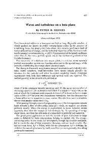
FIG. 1. Enhanced Geostationary Operational Environmental Satellite-10 (GOES-10) water vapor image and analysis of the 400-hPa PV field from the AVN Model at 0000 UTC 18 Feb 2001. The G-IV departed from its base in Hawaii and flew northward toward the southern end of the PV anomaly, and then took a more northeasterly track as it released dropsondes (black part of track).

The RUC-20 model configuration consisted of a 20-km grid resolution. In addition, a 13-km version of RUC was produced, but no results from this experiment are shown in this paper. Both models contained 50 hybrid isentropic sigma-coordinate levels. The isentropic framework is believed to be advantageous for the analysis of upper-level frontal systems. The National Centers for Environmental Prediction (NCEP) Aviation (AVN) Model supplied the external boundary conditions (by contrast, the operational version of the RUC model uses Eta Model boundary conditions). Other aspects of the RUC model configuration were TABLE 1. In situ data observation times* and levels for the G-IV aircraft. Time period of data (UTC 18 Feb 2001) 0000–0024 0030–0052 0101–0017 0122–0140

Flight level (ft) 41 33 35 37

000 000 000 000

(km)

(hPa)

12.5 10.1 10.7 11.4

175 260 235 214

* Times during which the aircraft underwent altitude change maneuvers are omitted, since data during such times are unreliable.

identical to the operational version (Benjamin et al. 2004a,b). Nested CH model domains were spawned at various times beginning at 1800 UTC from an 18-km version of the COAMPS model initialized at 0000 UTC 17 February, with the finest-scale domain being spawned at 0400 UTC 18 February. The CH model includes a Rayleigh friction absorber to reduce gravity wave reflections from the upper boundary, which was at 30 km. Of primary interest to the current study is the highest-resolution 1-km grid, which offered 50-m vertical resolution. Additional details about the CH and COAMPS model configurations are provided by Lane et al. (2004, hereafter L04). Resolution sensitivity experiments performed by L04 demonstrated that the simulated gravity waves in the upper-level front were robust and not spurious owing to possibly inconsistent vertical resolution relative to the horizontal resolution.

b. Upper-level front/jet system and tropopause structures The RUC model SCATCAT domain is shown in Fig. 2 along with a 1-h forecast of winds at 260 hPa valid at

NOVEMBER 2005

KOCH ET AL.

3889

FIG. 2. Domain of the special RUC model runs for the SCATCAT experiment showing 1-h forecast of wind barbs and isotachs at 260 hPa (33 000 ft) valid at 0100 UTC 18 Feb 2001 over the Pacific Ocean (note the Hawaiian and Aleutian Islands). Isotach values (kt) are shown in the color bar at the bottom of the figure (forecast maximum wind is 92 m s⫺1). Note that the G-IV flew from the core of a very strong jet streak to its cyclonic side. The white rectangle depicts the domain over which gravity waves were analyzed (Fig. 9). Also depicted is the location of the model cross sections appearing in Figs. 3 and 4 (white line), and that of a smaller segment over which the G-IV released dropsondes (black line, cf. Fig. 8). RUC model diagnostics appearing in Figs. 5 and 6 are computed over the southwest–northeast portion of the aircraft track.

0100 UTC 18 February. An intense 92 m s⫺1 jet maximum is apparent in the vicinity of the G-IV track, and an impressively strong cyclonic shear exists to its northeast. As this northwesterly jet streak approached the base of a sharp upper-level trough, noticeable diffluence developed in its exit region. Isentropic cross sections of Ertel PV perpendicular to the upper-level northwesterly flow from the RUC analysis at 2100 UTC and a 6-h forecast valid at 0300 UTC are shown in Fig. 3. The corresponding isotach vertical cross sections appear in Fig. 4. An intensifying upper-level jet and associated front can be discerned. As the forecast jet maximum increases from 83 to 92 m s⫺1 during this 6-h period, the associated horizontal and vertical wind shears intensify, particularly above the jet core near where the G-IV flew its circuit. The strengthening of the jet is directly linked to frontogenesis in the upper troposphere, as can be inferred from the increasing slope of the isentropic surfaces in the

250–350-hPa layer at 600 ⬍ x ⬍ 1400 km (and proven in section 4b). Also apparent in these cross sections is a warm front in the midtroposphere that links with the upper front aloft. However, the two fronts are distinct, as the warm front occurs on the back side of a deep cold dome seen in the rightmost part of the domain, whereas the upper-level front is a developing feature that propagates into the domain from the southwest (as emphasized by the highlighted 325-K isentrope). The strong static stability and impressive cyclonic shear along the warm front and the bottom part of the upper-level front together support a pronounced tropopause fold (1.5 PVU), which descends from 550 hPa at 2100 UTC (Fig. 3a) to 650 hPa by 0300 UTC (Fig. 3b). Also of interest is a secondary tropopause fold immediately above the primary fold. This secondary fold increasingly stretches out with time along a stable lamina near 350 hPa. The primary and secondary folds were both apparent in the initial state of the RUC model at

3890


VOLUME 62

FIG. 3. RUC vertical cross sections (cf. Fig. 2) of isentropes (2-K contours) and Ertel potential vorticity (1 PVU ⫽ 1 ⫻ 10⫺6 K kg⫺1 m2 s⫺1, PVU values given by color shading, see color bar) along a 2800-km path perpendicular to the jet stream flow. The cross section is from (a) the RUC analysis at 2100 UTC 17 Feb, and (b) the 6-h forecast valid at 0300 UTC 18 Feb. Vertical lines denote the ⬃400 km segment over which the G-IV took measurements. The 325-K isentrope is highlighted to emphasize the fluctuations associated with gravity waves 1, 3, and 5. Tropopause fold is defined by values of potential vorticity ⬎1.5 PVU.

2100 UTC. By contrast, there are several very finescale features in the PV field that seem to have developed in the forecasts. These tropopause undulations, which lie directly above the secondary fold (highlighted by the 325-K isentrope), are actually upward propagating gravity waves (note the tilt of the phase lines shown by the thick curves) and, as shown later, have strong counterparts in the dropsonde data analysis. The assertion

that the waves in the dropsonde data propagated upward is corroborated by L04 in their finding of anticyclonic rotation in a hodograph analysis of individual dropsondes. The hodograph method (Cot and Barat 1986) is derived from the polarization relation for a monochromatic inertial gravity wave. The dropsonde hodograph analysis indicated vertical and horizontal wavelengths of 1.6 ⫾ 0.4 km and 145 ⫾ 60 km, respectively.

FIG. 4. As in Fig. 3 except showing isotachs (5 m s⫺1 intervals, color shading) and isentropes (contours). Jet maximum value is (a) 83 m s⫺1 in the 2100 UTC 17 Feb analysis, and (b) 92 m s⫺1 in the 6-h forecast valid at 0300 UTC 18 Feb.

NOVEMBER 2005

KOCH ET AL.

Three gravity waves are analyzed at 0300 UTC in Fig. 3b, but a total of five appeared at one time or another from 2100 to 0300 UTC. These waves all existed in direct association with the developing upper-level front. The time-averaged vertical and horizontal wavelengths of 1.8 ⫾ 0.4 and 216 ⫾ 66 km are comparable to the dropsonde hodograph values, as well as to those seen in the COAMPS and CH model forecasts, despite the fact that the simulated jet maximum in this crosssection plane was ⬍80 m s⫺1 in those models and the lamina along which the secondary tropopause fold developed was not as well defined (see Figs. 4 and 7 in L04). Nevertheless, the gravity waves are a robust feature of all the models, and their existence did not depend appreciably upon either the initialization time or whether the 13- or 20-km version of RUC was used.

3. Turbulence diagnostic analyses a. Model diagnostics Three different measures of turbulence were computed from the models. First, the classical Miles– Howard condition for shearing instability is that Rig ⫽ N2ⲐS2 ⬍ 1Ⲑ4,

共1兲

where S is the vertical wind shear [(⳵u/⳵z) ⫹ (⳵␷ /⳵z) ] and N is the Brunt–Väisälä frequency. The second parameter is the DTF3 algorithm (Marroquin 1998), which is one of the members of the GTG/ITFA suite of RUC-based turbulence algorithms. DTF3 is based on the assumption that the dissipation rate of TKE(␧) is in steady state, which may be expressed as 2

␧ ⫽ Km关c1S2 ⫺ c2共N2ⲐPr兲兴,

2 1/2

共2兲

where Km is the eddy diffusivity coefficient for momentum, Pr is the Prandtl number, and c1 and c2 are constants. Given the flux form of the Richardson number, Ri f ⫽

Kh Ri , Km g

共3兲

it can be shown that the TKE as defined by the DTF3 formulation is simply DTF3 ⫽ 共0.7K mⲐN兲S2共0.75 ⫺ 0.52Ri f兲.

共4兲

The third turbulence diagnostic to be presented is the subgrid TKE computed in the CH model assuming Pr ⫽ 1 and using the formulation of Deardorff (1980), TKE ⫽ 共10K m Ⲑ l 兲2,

共5兲

where l ⫽ ⌬z ⫽ 50 m is the mixing length. Since Km ⬀ (1 ⫺ Rif)1/2 for Rif ⬍ 1, it may be inferred that subgrid TKE exists whenever Rif ⬍ 1 (or Rig ⬍ 1 since Pr ⫽1).

3891

Isotach and DTF3 fields are shown in a vertical cross section over the ⬃500 km length covered by the G-IV dropsonde releases in the 3-h RUC forecast valid at 0000 UTC 18 February in Fig. 5a and the 0000 UTC RUC analysis that included the assimilation of the dropsonde data in Fig. 5b. DTF3 maxima appear in the regions of strong vertical wind shear directly above and below the jet core. This is not altogether surprising since, according to (4), DTF3 is proportional to the square of the shear [areas where DTF3 ⬎ 3.0 m2 s⫺2 (shaded) correspond to MOG turbulence]. It is also readily apparent that DTF3 is enhanced for the stronger jet analysis appearing in Fig. 5b. The cross section of Rig at 0000 UTC 18 February computed from the RUC analysis excluding the dropsonde data is shown in Fig. 6a; this may be compared to the Rig field computed from the RUC analysis that assimilated the dropsonde data (Fig. 6b), and to that computed directly from the dropsonde data in the absence of RUC model background fields (Fig. 6c). Although the same basic patterns are evident, generally mirroring those seen in the DTF3 fields, the RUC analysis of turbulence parameters suffers in the absence of the dropsonde data, as considerably more area is covered by Rig ⬍ 0.50 in the RUC analysis that included these data (which itself shows a smaller region of Rig ⬍ 0.50 than the analysis of the dropsonde data alone in Fig. 6c). The influence of the dropsonde data on the RUC analysis is likely exaggerated relative to what might be expected to be the case over the datarich CONUS, where much more data exist to produce better RUC analyses of the shear and stability fields. Nevertheless, these comparisons serve to demonstrate the strong sensitivity of the Rig calculations to the data provided to the model initial analysis. The spatial structure of the DTF3 fields is very revealing. A strikingly banded nature to the DTF3 fields at 33 000 ft (10.1 km) is apparent in the 6-h RUC forecast for 0300 UTC (Fig. 7b). The bands are parallel both with the flow and with an intensifying frontal zone just to their west, as seen in the packing of the isotherms at 275 hPa and the diagnosis of strong frontogenesis in a band oriented parallel to the narrower DTF3 bands (Fig. 7a). Similar bands were evident at the 35 000- and 37 000-ft flight levels (not shown), and at other times, though the banding was less apparent at earlier times. It is shown below that these bands in DTF3 are directly coupled to the gravity waves mentioned earlier (Fig. 3). Similar patterns appear in the subgrid TKE and perturbation potential temperature (␪ ⬘) fields on constantheight surfaces in the 1-km resolution CH model (note the location of this model domain as depicted by the

3892


VOLUME 62

FIG. 5. Vertical cross sections of DTF3 diagnostic turbulence predictor fields (shaded) and isotachs (5 m s⫺1 contours) computed from the RUC model (a) 3-h forecast verifying at 0000 UTC and (b) initial analysis at 0000 UTC 18 Feb that includes dropsonde data. DTF3 ⬎ 3.0 and 4.0 m2 s⫺2 is shown with light (dark) shading, respectively, corresponding to moderate and severe levels of predicted turbulent kinetic energy. Cross-section path (southwest–northeast portion of black line in Fig. 2) is the same as that used for the dropsonde analysis in Fig. 8.

small box in Fig. 7a). The ␪ ⬘ field displays bands with a wavelength of ⬃180 km and the TKE and Ri fields are directly associated with these features in both the horizontal plane (Fig. 7c) and in a vertical cross section taken from the 3-km resolution version of the CH model in a direction perpendicular to the bands and the general flow direction (Fig. 7d). Bands of wave-induced Ri ⬍ 1 (associated with subgrid turbulence) in this vertical plane are evident above 10 km. L04 shows that these TKE and Ri bands were the result of gravity wave modulation of the background shear and stability fields, which reduced the Richardson number within the low static stability phase regions of the gravity–inertia waves, resulting in parallel bands of reduced Ri (thus, increased TKE). Therefore, the regions of (parameterized) turbulence are directly related to the gravity waves despite the fact that the CH model did not directly simulate MOG turbulence at the resolvable scales of motion; rather, TKE arose entirely from the subgrid parameterization scheme.

b. Dropsonde vertical cross-section analysis Isotachs, isentropes, and DTF3 fields were computed from the quality controlled and lightly filtered dropsonde data (Fig. 8). Data were interpolated between the flight level measurements (176 hPa) and the level at which the falling sonde reached thermal equilibrium

with its environment (⬃200 hPa); thus, details at the very top of the cross section should be viewed with some caution. An extremely intense jet core exceeding 100 m s⫺1 is analyzed. This value is comparable to the 92 m s⫺1 in the RUC 1-h forecast (Fig. 4). Other features evident in the dropsonde cross-section analysis that are also seen in the model fields include the upward sloping layer of strong static stability defining the warm front, the sharp tropopause along which the upper-level front developed in the RUC model (note that the dropsonde cross section is confined to the narrow window denoted by the two parallel vertical lines in Fig. 3), and the strong correspondence between the observations of high DTF3 (yellow and red shaded regions) and the DTF3 diagnosed from the RUC model forecasts (Fig. 5). The dropsonde cross-section analysis also suggests the presence of vertically propagating gravity waves above the jet core and to its cyclonic (northeastern) side in the lower stratosphere. Their horizontal wavelength of ⬃120 km, which is barely resolvable by the 40-km dropsonde spacing, is somewhat smaller than the mean value of 216 km derived from the RUC-20 (and RUC-13) model and the 180 km seen in the CH model results. Of particular note is the occurrence of aircraftdetected MOG turbulence patches (the yellow parts of the flight tracks displayed in Fig. 8). This turbulence is in close proximity to diagnosed regions of high DTF in

NOVEMBER 2005

3893

KOCH ET AL.

that part of the atmosphere directly affected by the gravity waves (excluding the analysis above 200 hPa, where the possible existence of gravity waves cannot be corroborated since the dropsondes were not in thermal equilibrium with the environment).

4. The relationship of gravity waves to potential vorticity structures and ozone In this section, we first discuss the dynamical cause for the gravity waves, and then explore interrelationships between the waves, the tropopause folds and PV structures, and ozone fluctuations.

a. Gravity waves as the probable cause for the banded structures The wavelike features seen in the RUC model cross sections (Fig. 3) appear as propagating waves in the pressure field on the 325-K isentropic surface (Figs. 9a,b). The average phase velocity C for the five waves analyzed in the cross sections and the isentropic maps is 21.0 m s⫺1 from 230°. These waves are fully exposed in a spatial wavelet analysis (Morlet et al. 1982) of the 200-km-scale pressure waves (wave packet A in Fig. 9c). The Morlet wavelet analysis also reveals other waves in the south central part of the domain displaying a southeast wave vector (wave packet B), which occur above the low-level cold front. Packet A bears closest similarity to mode 3 in the idealized modeling study of Zhang (2004), whereas packet B is similar to mode 2. Whether all these features are, in fact, gravity waves can be addressed by considering the wave dispersion and polarization equations. The perturbation horizontal and vertical velocities for a vertically propagating inertia–gravity wave are respectively (e.g., Gossard and Hooke 1975; Gill 1982) u⬘ ⫽

m␻i

and w⬘ ⫽ i

FIG. 6. Vertical cross sections of Richardson number (Rig) at 0000 UTC 18 Feb 2001 from (a) the RUC analysis without any dropsonde data, (b) the RUC analysis including all the dropsonde data, and (c) an analysis of the dropsonde data. Values of Rig ⬍ 1.50, 1.00, 0.50, and 0.25 are shown in blue, green, yellow, and red shading. Cross-section location is shown by the G-IV path in Fig. 2.

␻i 2

N

g

␪⬘ ␪

g

kN2

⫽⫺

冉

␪⬘

共6兲

␪

␻i2 ⫺ f 2 N ⫺ 2

␻i2

冊

1Ⲑ2

u⬘,

共7兲

where k ⫽ 2␲/␭x is the horizontal wavenumber, ␻i is the intrinsic frequency, i ⫽公⫺1, f is the Coriolis parameter, and ␪ and ␪ ⬘ are the mean and perturbation potential temperatures. Equation (7) shows that the vertical velocity field is in quadrature phase with the potential temperature field. The intrinsic frequency can be determined from the dispersion equation applicable to rotating hydrostatic waves, 2 ␻i1 ⫽f2⫹

N2k2 m2

.

共8兲

3894


VOLUME 62

FIG. 7. (a) Virtual potential temperature (2°C isotherms, black contours), frontogenesis function [color shading, intervals of 5 K (100 km)⫺1 (3 h)⫺1] and wind vectors at 275 hPa from RUC analysis at 0000 UTC 18 Feb; (b) DTF3 at 33 000 ft (10.1 km, 260 hPa) from 6-h RUC forecast valid at 0300 UTC, (c) subgrid TKE and perturbation potential temperature from value of 335 K (0.5-K interval, solid ⫽ positive, dotted ⫽ negative) at 11 km MSL at 0600 UTC from CH 1-km domain model shown by the small black box in (a), and (d) cross section of Richardson number and potential temperature (2-K intervals) fields from CH model along the southwest–northeast diagonal through the small black box. Black lines in (a) denote locations of RUC cross sections (long segment) and NE–SW part of the G-IV track (short segment); yellow line through the small black box depicts location of CH model cross section shown in (d). Horizontal line in (d) depicts location of 11-km altitude plot in (c). Light pink and red shading in (b) represents DTF3 ⱖ 3.0 and 4.0 m2 s⫺2, corresponding to moderate and severe levels of turbulence, respectively. The red shading in (c) is linear with the maximum value of 0.2 m2 s⫺2 denoted by the darkest shade.

Alternatively, intrinsic frequency can be obtained from the wave vector method, using the ground-relative frequency ␻ according to

␻i 2 ⫽ ␻ ⫺ U · k.

共9兲

Application of (6)–(9) to the RUC model crosssection fields produced the results summarized in Table 2 for wave packet A. The two estimates of the intrinsic frequency agree within 37% of one another, which we consider supportive of the gravity wave interpretation given the variability in the wavelengths and the degree of representativeness of the mean wind in the wave layer. Also, the predicted perturbation wind speed

(3.0 m s⫺1) is consistent with that seen in the model fields (Fig. 4b). Finally, another criterion examined here is the upper inertial critical level Zc1, defined as the level at which a vertically propagating inertia–gravity wave is dissipated. This level is given as the altitude where the wind in the plane of wave propagation is U ⫽ C ⫹ f/k. We estimate Zc1 ⫽ 148 hPa, consistent with the limit to the upward propagation behavior of the waves seen in the model cross sections (Fig. 3b and 7d, also see Fig. 5 in L04).

b. Mesoscale diagnostic analyses Gravity wave packet A was triggered in a region of unbalanced flow very near to the G-IV path (Fig. 10a).

NOVEMBER 2005

KOCH ET AL.

3895

FIG. 8. Vertical cross section of wind speed (blue lines, 5 m s⫺1 isotachs), potential temperature (black lines, 2-K isentropes), and DTF3 turbulence diagnostic (shading) computed from dropsondes (note release times at bottom of display) released from 2326 UTC 17 Feb to 0024 UTC 18 Feb. Jet core winds in excess of 80 m s⫺1 are highlighted (maximum of 100 m s⫺1). Yellow and red shading, respectively, depicts DTF3 values in excess of 3.0 and 4.0 m2 s⫺2. Also shown are the four stacked legs of the G-IV tracks (black lines with arrows depicting sense of aircraft travel), and those segments of the legs (yellow highlighting) for which moderate-or-greater turbulence was diagnosed in the flight-level data (see text). The DTF3 fields should be compared to the observed turbulence areas. This analysis should be compared with those derived from the RUC forecasts in Figs. 4 and 5. Note distance scale at top of display. The vertical line depicts where the G-IV switched directions from northerly to northeasterly (Fig. 1).

Imbalance was diagnosed as the residual of the nonlinear balance equation computed from the raw RUC hybrid coordinate data in a manner discussed by Koch and Caracena (2002). Although other measures of imbalance have been proposed, the nonlinear balance equation method seems to produce the most robust and general results (Zhang et al. 2000). Similar to the idealized modeling studies of Reeder and Griffiths (1996) and Zhang (2004), the imbalance occurred in the vicinity of the tropopause fold (Figs. 10d,e). However, in the present case, the imbalance was actually maximized where the secondary tropopause fold joined with the primary fold (near the intersection of the 300-hPa level with the rightmost vertical line in Fig. 3b). The existence of the gravity waves directly above the sec-

ondary tropopause fold and immediately downstream of the region of strong upper-level frontogenesis (Fig. 10d) thus appears to have been more than just a coincidence. Nonetheless, we investigated another possible mesoscale forcing for the bands—conditional symmetric instability (CSI), which arises when a saturated atmosphere is made symmetrically unstable due to the release of latent heat. The primary motivation for examining this issue is that CSI is manifested as slanted roll circulations with their axes oriented along the thermal wind vector (Bennetts and Sharp 1982; Xu 1992; Koch et al. 1998). In the present case, this direction would be essentially along the flow, a characteristic that is displayed by the bands. The existence of CSI can be

3896


VOLUME 62

determined either by using the parcel method (Emanuel 1983a,b), by finding whether there are any regions where moist Ertel PV is negative in a cross section taken perpendicular to the thermal wind (Moore and Lambert 1993; Koch et al. 1998), or by computing the three-dimensional, saturated equivalent geostrophic potential vorticity (Schultz and Schumacher 1999) defined as *. MPV* g ⫽ g ␩g · ⵱␪ e

FIG. 9. (a) Pressure (5-hPa intervals) on the 325-K isentropic surface in the initial RUC analysis for 2100 UTC 17 Feb over the zoomed-in area depicted as a white rectangle in Fig. 2; (b) as in (a), except for a 6-h forecast valid at 0300 UTC 18 Feb; and (c) wavelet analysis of the 325-K pressure field from a 4-h forecast valid at 0100 UTC over a larger domain showing features with 200-km wavelengths. Location of wavelet domain can be understood by observing the G-IV and RUC cross-section lines (cf. Fig. 2). Gravity waves are denoted by numbers 1, . . . , 5. Two wave packets are revealed in the wavelet analysis: packet A is the region of concentrated study near the aircraft track, and packet B comprising waves with northeast–southwest orientations is near the surface cold front.

共10兲

Here, ␪ e* is the saturated equivalent potential temperature and ␩g is the absolute geostrophic vorticity. We employed the MPV* g method since it avoids the issue of how to orient the cross section when directional shear is present. The resulting analysis (Fig. 10b) suggests regions susceptible to CSI only in the vicinity of wave packet B near the surface cold front. Thus, we can rule out the possibility that CSI might explain the bands in wave packet A in the vicinity of where the G-IV flew. In light of the evidence presented that wave packet A represents inertia–gravity waves forced by unbalanced dynamics near the tropopause, rather than CSI, it is of interest to understand how such imbalance may have arisen. Examination of the ageostrophic winds (Fig. 10c) reveals flow directed toward higher heights in the exit region of the jet streak (Fig. 2)—this being the signature of a thermally indirect transverse circulation (near 32°N, 155°W). Likewise, a thermally direct circulation in the jet entrance region exists ⬃1000 km to the northwest of the upper-level front. However, streamwise ageostrophic flow attributable to the effects of curvature is of greater relevance to the generation of the frontogenesis shown in Fig. 10d. The effect of flow curvature on the ageostrophic flow is suggested in the vicinity of the downstream trough near the eastern edge of the RUC domain where a slight upstream-directed component can be discerned in association with the thermally indirect circulation. Likewise, in the vicinity of the upstream ridge, supergeostrophic flow causes the ageostrophic winds to display a downstream component. The product of these diametrically opposed wind regimes is strong confluence in the alongstream ageostrophic flow in the vicinity of the upper-level front, and the creation of a favorable environment for ageostrophically forced alongstream frontogenesis and streamwise vorticity advection. The resultant along-jet cold advection in the presence of cyclonic horizontal shear would shift the thermally direct ageostrophic circulation in the jet entrance region toward the anticyclonic side of the jet axis. Consequently, the region of maximum subsidence became located directly beneath the jet axis (not shown)—a pattern that is highly frontogenetical with respect to the vorticity field (Keyser

NOVEMBER 2005

3897

KOCH ET AL. TABLE 2. Mean inertia–gravity wave properties computed from RUC-20 model grids.*

Symbol

Wave parameter

Units

Mean ⫾ std dev

␣ C CX ␭X ␭Z ␻ f U ⌵ ␻i1 ␻i2 ␪⬘ u⬘ w⬘ Zc1

Wave phase direction Wave phase speed Phase speed in wave plane Horizontal wavelength Vertical wavelength Wave frequency Coriolis parameter Mean wind in wave layer Brunt–Väisälä frequency Intrinsic frequency (8) Intrinsic frequency (9) Perturbation potential temperature Perturbation horizontal wind Perturbation vertical velocity Upper inertial critical level

° m s⫺1 m s⫺1 km km s⫺1 s⫺1 m s⫺1 s⫺1 s⫺1 s⫺1 K m s⫺1 cm s⫺1 m s⫺1, hPa

230 ⫾ 10 21.0 ⫾ 6.6 16.1 ⫾ 6.3 216 ⫾ 66 1.8 ⫾ 0.4 6.23 ⫾ 1.07 ⫻ 10⫺4 9.35 ⫻ 10⫺5 10 ⫾ 6 2.23 ⫻ 10⫺4 2.18 ⫾ 0.44 ⫻ 10⫺4 3.48 ⫾ 0.91 ⫻ 10⫺4 1.5 ⫾ 0.6 3.0 ⫾ 1.5 3.2 ⫾ 1.6 19.3, 148

* Estimates for u⬘ and w⬘ use the average of the two methods for determining the intrinsic frequency expressed by (8) and (9).

and Shapiro 1986). This positive feedback loop between frontogenesis and increasing subsidence along the jet axis is a process that is conducive to tropopause folding and unbalanced frontogenesis and, thus, to the generation of gravity–inertia waves. Indeed, vertical cross sections oriented normal to the jet axis (Figs. 10e,f) show intensifying frontogenesis along the cyclonic shear side of the upper-level frontal zone above 300 hPa, whereas frontogenesis along the lowto-mid tropospheric front actually weakens with time. Amplification of the gravity–inertia waves in the CH model coincided with this intensification of the upperlevel front, as discussed more fully by L04.

c. Interrelationships between ozone fluctuations and other variables Comparisons were made between flight-level observations and fields analyzed from the RUC-20 model simulation using RUC model “meteograms.” The method for deriving the meteograms consisted of three steps. First, the three-dimensional model grid data were interpolated to the plane of the cross section at 10-km intervals. Next, the 25-mb resolution model data were vertically interpolated to the constant-height altitudes flown by the aircraft. Finally, a space-to-time conversion was performed under the assumption of stationarity for the duration of each flight leg (i.e., meteograms were created by taking the beginning and end times for each flight leg as the times for the endpoints of each model cross section). An example of this procedure appears in Fig. 11, which compares time series of 1) potential temperature derived from the RUC model forecast fields and as measured by the aircraft and 2) model PV values versus aircraft-measured ozone. The

meteograms in Fig. 11b show a general increase of potential temperature as the cyclonic (left exit) region of the jet is approached in both the observations and the model, reflecting the fact that the aircraft was traveling from the upper troposphere into the lower stratosphere. The reverse sequence is evident at the 33 000-ft level (Fig. 11a). At both levels, variations in the G-IV observations occurring at scales smaller than ⬃7⌬x (where ⌬x is the 20-km RUC resolution) are clearly absent in the model. Isentropic PV and ozone are conserved quantities serving as passive tracers of airmass exchange processes. Large ozone levels on the order of 400–800 ppbv are seen in the layer between 33 000 and 41 000 ft. The ozone values are largest at 41 000 ft (above the jet core) and at the northeast ends of both flight legs. This is consistent with the conjecture that the aircraft was penetrating a tropopause fold as it entered the lower stratosphere in its northeastward travel (cf. to the RUC crosssection analysis in Fig. 3). Fluctuations in G-IV ozone and potential temperature are highly correlated at 33 000 ft (Fig. 11a). The RUC potential temperature curve is comparable to the overall trend in the G-IV data at that level. Similarly, the RUC PV and aircraft ozone data show a general trend downward as the aircraft approached the jet core from its cyclonic side, and both traces also indicate two large-scale rises in the time series, cresting at ⬃0039 and 0047–0050 UTC. The dropsonde cross-section analysis (Fig. 8) shows that the aircraft was penetrating a pronounced gravity wave at this time immediately to the northeast of the high DTF3 region (260 hPa). Close inspection of the G-IV time series in Fig. 11a suggests the appearance of considerably greater high-frequency energy begin-

3898


VOLUME 62

FIG. 10. Mesoscale diagnostic analyses performed from RUC model fields: (a) unbalanced flow regions diagnosed from the residual of the nonlinear balance equation [intervals of 2 ⫻ 10⫺8 s⫺2, positive (negative) regions denoted by solid (dotted) contours] on the 325-K isentropic surface (pressure is indicated by black contours at intervals of 4 Pa) for the 3-h forecast valid at 0000 UTC 18 Feb; (b) regions of negative moist geostrophic potential vorticity on the 325-K isentropic surface from the 3-h forecast valid at 0000 UTC 18 Feb; (c) absolute vorticity (blue contours, 10⫺5 s⫺1), ageostrophic wind vectors, and geopotential height (60-m intervals, red contours) at 275 hPa from the 0000 UTC 18 Feb RUC analysis; (d) potential vorticity (PVU), contours, ageostrophic wind vectors, and frontogenesis function [color shading, K (100 km)⫺1 (3 h)⫺1] from the RUC analysis at 0000 UTC 18 Feb; (e) vertical cross section of potential vorticity (PVU, color shading), isentropes (2-K intervals), and frontogenesis function [K (100 km)⫺1 (3 h)⫺1] from the analysis at 0000 UTC 18 Feb; and (f) as in (e) except from the 3-h forecast valid for 0300 UTC 18 Feb. The locations of the RUC cross sections shown in (e) and (f) and G-IV tracks are depicted by the long line segments in (a)–(d).

ning at ⬃0444 UTC. In fact, the G-IV in situ data indicated MOG turbulence beginning at this time (note the lowest-level yellow segment of the aircraft track in Fig. 8.)

Wild fluctuations in ozone and G-IV potential temperature were measured at the 41 000-ft level, but neither variable appears to relate well to either the RUC model variables or to each other. Fluctuations in the

NOVEMBER 2005

KOCH ET AL.

FIG. 11. Time series of potential temperature derived from RUC model forecast fields (triangles) and as measured by the G-IV aircraft (heavy lines), RUC potential vorticity (dots), and ozone measured from the G-IV (light lines). RUC values are computed using the meteogram technique discussed in the text. (a) Analyses at FL330 were taken from 0030 to 0054 UTC 18 Feb as the aircraft flew from the cyclonic (northeastern) side of the upper-level jet to its core, whereas those at (b) FL410 were taken from 2345 UTC 17 Feb to 0025 UTC 18 Feb in the opposite direction. Note the times of diagnosed MOG turbulence, gravity waves, and the frontal zone, as well as the scale at the top of the figure (obtained by converting time to space using a true airspeed of 230 m s⫺1).

3899

3900


VOLUME 62

FIG. 12. Time series of turbulence variables showing onset of MOG turbulence at 0043 UTC and sporadic bursts of turbulence thereafter. Blue plot represents the 1-Hz GPS Honeywell vertical velocity data; red plot is for the 25-Hz aircraft vertical acceleration data for the entire four flight legs of the mission, beginning at 12.5 km (41 000 ft), followed by legs at 10.1 km (33 000 ft), 10.7 km (35 000 ft), and 11.4 km (37 000 ft).

RUC PV field do not relate as well to the aircraft ozone variability as they had at the lower altitude. Ozone and potential temperature observations at the intermediate flight altitudes (35 000 and 37 000 ft) bore a strong relationship with one another and with trends in the respective RUC model variables (not shown). As will be discussed next, MOG turbulence was not reported on the 41 000-ft flight leg, was quite pronounced on the 33 000-ft and 35 000-ft legs, and was intermediate on the 37 000-ft leg. We take these facts to mean that the rapid fluctuations in ozone at 41 000 ft represent fossil turbulence or remnants of earlier stratosphere– troposphere turbulent exchange processes, whereas the fluctuations at lower levels represent currently active turbulence.

5. Spectral, wavelet, and structure function analyses of the flight-level data Autospectral analyses were conducted to determine the dominant frequencies and wavelengths of the gravity waves and their relationship to turbulence. Crossspectral analyses provided an understanding of the phase relationships between variables needed for proper determination of which spectral signals are manifestations of gravity waves and which represent turbulence. Wavelet analyses were performed to overcome the natural limitations imposed by the “global”

nature of spectrum analysis. The spectral energy transfer process was investigated using third-order structure function analysis.

a. Autospectral analyses Composite time series from the four flight levels of 25-Hz aircraft vertical acceleration and 1-Hz vertical velocity data are shown by the red and blue traces in Fig. 12, respectively, for the entire 2340–0140 UTC period of G-IV observations. Both traces suggest that negligible turbulence was encountered at the 12.5-km (41 000 ft) flight level. MOG turbulence first appears at 0043 UTC at the 10.1-km (33 000 ft) level and dominates the remainder of the record at that altitude and also at the 10.7-km (35 000 ft) level. Last of all, a short burst of MOG turbulence from 0128–0131 UTC appears at the 11.4-km (37 000 ft) level (this corresponds to 41.4-km spatial distance, given the aircraft true airspeed). The largest spikes in the vertical acceleration data approach 0.5 g force (4.9 m s⫺2). Although these time series are suggestive of when turbulence is encountered, they do not provide information about the interactions between gravity waves and turbulence. Most previous investigations of atmospheric wave–turbulence interactions have employed spectral methods (Gage 1979; Nastrom and Gage 1985; Bedard et al. 1986; Chan et al. 1998). The 25-Hz aircraft potential temperature, longitudinal (alongflight) wind,

NOVEMBER 2005

KOCH ET AL.

3901

ertial subrange (note the slanted line). Atmospheric wind and temperature spatial spectra at middle latitudes and upper levels exhibit a k⫺5/3 behavior for scales ranging from ⬃400 km down to 1 km (Gage 1979; Lilly 1983; Nastrom and Gage 1985; Cho and Lindborg 2001), though recent measurements collected from research aircraft show an extension of this spectral behavior down to scales as small as 40 m (Gultepe and Starr 1995; Frehlich and Sharman 2004).

b. Cross-spectral analyses

FIG. 13. Power spectral analysis of aircraft vertical acceleration data for the 10.1-km flight altitude for 0030–0042 UTC (dark curve) and 0043–0050 UTC (light curve). Spectral peaks 1, 2, and 3 at 0.07, 0.65, and 6.0 Hz correspond to horizontal wavelengths of 3.3 km, 350 m, and 38 m, respectively. Each of these peaks is bandwidth-separable and statistically significant at the 95% threshold. The diagonal line represents the ⫺5/3 spectral slope characteristic of atmospheric spectra in the inertial subrange.

transverse (crossflight) wind, and aircraft vertical acceleration data were subjected to a fast Fourier transform (FFT) spectral analysis. Only constant-altitude samples not containing abrupt changes in aircraft heading, pitch, and roll were used. Adjacent sample windows were overlapped by 50%, and a Hanning window function was applied to the data to minimize high frequency aberrations caused by convolving the data segments with the window function. Figure 13 displays power spectra of the vertical acceleration data for 0030–0042 UTC (when there was an absence of MOG turbulence) and 0043–0050 UTC (when one of the strongest and most persistent turbulence events occurred). Two strong peaks appear in both spectra at f ⫽ 0.07 and 6 Hz, corresponding to spatial wavelengths of 3.3 km and 38 m. The former value is representative of the shorter end of the gravity wave spectrum for this case. The latter peak is related to an electronics noise problem on the aircraft, which persisted for the entire duration of the experiment; since the noise did not contaminate other spectral components, it could safely be ignored. A third significant peak (labeled “2”) appears only during the turbulent episode—the one at 0.65 Hz (corresponding to a wavelength of 350 m). This peak falls at the lower frequency end of the k⫺5/3 spectral slope region defining the in-

Cross-spectral analyses were performed after first removing the electronic noise problem by conservatively smoothing features with f ⬎ 1 Hz. Equal-log averaging of the highest frequencies produced the desired removal of noise energy. Use of a difference filter applied to the raw time series reduced the problem of leakage associated with red-noise (low frequency) variance in the data (Jenkins and Watts 1968). Analysis of statistical significance was performed for all spectral plots. An example of a coherence spectrum (a correlation analysis in the frequency domain) of potential temperature and the longitudinal wind for the 10.1-km flight leg appears in Fig. 14a. High coherence is found (significant at the 95% level) for four spectral peaks in this case, which correspond to horizontal wavelengths of 11.2, 4.6, 1.6, and 0.7 km. A strong in-phase covariance (90° phase angle) is demonstrated in the resultant phase spectrum for these peaks (Fig. 14b), which is consistent with the polarization relation for internal gravity waves [Eq. (6)]. This methodology was applied to cross-spectral analyses of the following variables: potential temperature and the longitudinal wind; potential temperature and the transverse wind; and potential temperature and the GPS aircraft vertical velocity data, for each of the flight legs for the time periods mentioned earlier. A summary of the significant peaks found in both the power spectral and coherence analysis results is given in histogram form in Fig. 15a, and the corresponding phase angles are summarized in Fig. 15b. Whether autospectral or cross-spectral methods are examined, the result is basically the same: a spectrum of gravity wave activity with wavelengths of 0.7–20 km occurred at all four flight levels, though considerably less so at the 41 000-ft flight level, where Ri was larger and DTF3 smaller than threshold (Figs. 7d, 8). Phase angles computed from the cross-spectra for potential temperature and longitudinal velocity are highly concentrated near 0° and, to a lesser extent at 180°, a result that is consistent with the polarization Eq. (6) for gravity waves. These results support and extend (in wavenumber

3902


FIG. 14. Cross-spectral analysis of 25-Hz potential temperature and longitudinal wind for the 10.1-km flight leg from 0030 to 0052 UTC: (a) coherence spectrum analysis; (b) phase spectrum analysis. Spectra are depicted over a portion of the entire frequency spectrum (Nyquist frequency 12.5 Hz). Highlighted peaks are statistically significant at the 95% level after accounting for the coherence bias factor (peaks ⬎0.73 are significant).

space) the findings from the dropsonde and model analyses of gravity waves.

c. Wavelet analyses Spectral approaches do enable separation of waves from turbulence, but they are valid only in a global

VOLUME 62

FIG. 15. Histogram plots of (a) statistically significant peaks in autospectra of potential temperature, longitudinal velocity, and transverse velocity (dark shading) and coherence spectra between potential temperature and longitudinal velocity (light shading), and (b) phase spectra of potential temperature and longitudinal velocity.

sense because a sufficiently long record characterized by statistical stationarity is required. Since spectral analysis can only provide such nonlocal information, and does not work well for small-amplitude waves, waves of short duration, or nonmonochromatic waves, it is not well suited to the study of intermittent, nonstationary phenomena such as turbulence, which displays

NOVEMBER 2005

KOCH ET AL.

rapid changes in phase, amplitude, and statistical properties. Direct observation of the turbulence generation mechanism, the intensity of the turbulence as a function of the wave amplitude, and its distribution in space and time is needed. Wavelet analysis has only recently begun to be used for the study of wave–turbulence interactions (Demoz et al. 1998), though it has been used previously to study the fractal nature of turbulent energy transfer (Mandelbrot 1975; Argoul et al. 1989). Wavelet analysis is capable of resolving localized structures in the time–frequency domain up to the limit imposed by Heisenberg’s uncertainty principle. The wavelet transform coefficients provide information about both the amplitude and phase of the fluctuations at each time and frequency and, therefore, should be able to provide understanding of the evolving relationship between wave and turbulence characteristics. Continuous wavelet analysis was applied to the horizontal wind, temperature, and vertical acceleration data obtained from the G-IV. For the transformation kernel function in the wavelet analysis, we used the continuous Morlet wavelet, which is a nearly orthogonal plane wave function modulated by a Gaussian envelope of unit width and normalized with zero mean (Morlet et al. 1982). The transform coefficients provide information about both amplitude and phase of the analyzed data. Comparison of the 0031–0051 UTC interval in the wavelet results (Fig. 16a) to the autospectra (Fig. 13) reveals that the low-frequency mode ( f ⫽ 0.06 Hz) seen in the 0043–0050 UTC spectrum actually consisted of multiple modes appearing sporadically during this interval. An important issue can be addressed with wavelet analysis—the prediction from linear theory (Weinstock 1987) that the amplitude of the turbulence should be correlated with the amplitude of the progenitor gravity waves, such that the turbulence intensity oscillates with the wave period. The wavelet results were used to reconstruct the gravity waves in the f ⫽ 0.06–0.09-Hz band (wavelengths of 3.8–7.7 km). Comparison of the resulting analysis (Fig. 16c) to the time series of turbulent intensity in the 0.3–0.9-Hz band (wavelengths of 0.2–0.8 km) shown in Fig. 16d reveals in a direct way that the times of occurrence of the strongest gravity wave amplitudes and the appearance of episodes of high turbulence energy were indeed highly correlated. This behavior is particularly impressive during the extensive 0103–0110 UTC turbulence/wave episode (which extended for nearly 100 km). Closer inspection reveals that the higher-frequency gravity waves tended to occur in packets defined by wave envelopes of various sizes ranging from 7–20 km (Fig. 16e), and it is with

3903

these wave packets that the turbulence intensity strongly correlated. The mechanism for turbulence production is related to nonlinear advection, which causes the wave front to become steeper with increasing amplitude until it breaks, at which point energy flows from the primary wave into harmonics down to turbulence (Weinstock 1986, 1987). The following characteristics help to distinguish waves from turbulence (Busch 1969; Stewart 1969): 1) waves propagate according to a dispersion relation, whereas turbulence is dissipative, diffusive, and random, and 2) the vertical velocity and potential temperature fluctuations are 90° out of phase for wave motions, but not for turbulence. Short-period gravity waves (in which the effects of the earth’s rotation are negligible) display a linear polarization between the two components of horizontal perturbation winds (phase angle ␸ ⫽ n␲, where n ⫽ 1, 2, . . .), as opposed to inertia–gravity waves, which display an elliptical polarization relationship. Lu et al. (2005) used this fact to reconstruct the waves in the current case in different frequency bands, doing so by combining knowledge of the dominant wave frequencies obtained from the cross-spectral analysis with the localized information from the wavelet analysis. Their analysis confirms our conjecture that the gravity waves occurred in packets of 0.5–1.5-min duration (⬃7–20 km distance). Another interesting question concerns whether static instability (buoyancy) or dynamic instability due to vertical shear augmented by the passage of the gravity waves was the more important source for turbulence. If static instability was the dominant source, then maximum turbulent intensity should occur at the nodal surfaces of the wave (halfway between the wave crests and troughs). However, if dynamic instability was the more important source, turbulence should be greatest at the crests and troughs. During each gravity wave interval (defined by the period of time between successive wave troughs), the phase of the wave at which the maximum turbulent intensity occurred was plotted (Fig. 16b). Results indicate that turbulence intensity did not vary systematically with wave phase; thus, at least in the present case, the wavelet analysis supports the concept that the wave–turbulence process involves both dynamic and convective instabilities.

d. Structure function analyses Neither the power spectrum nor the wavelet approach can resolve the longstanding controversy about the nature of the kinetic energy cascade in the scales from the mesoscale to the inertial subrange, where the spectrum takes the form described by Kolmogorov (1941) as

3904


VOLUME 62

FIG. 16. Wavelet analysis of aircraft vertical acceleration data: (a) time–frequency display of wavelets (m s⫺2) at 10.1-, 10.7-, and 11.4-km altitudes; (b) phase ␸W of gravity waves (degrees) at which maximum turbulence intensity occurred (only if larger than 0.5 m2 s⫺4); (c) amplitude AW (m s⫺2) of gravity waves reconstructed from wavelet analysis for the 0.06–0.09-Hz frequency band; (d) turbulence intensity AT (m2 s⫺4) at a frequency of 0.65 Hz; (e) zoomed-in display of (b)–(d) for the period 0106–0110 UTC showing three wave packets (envelopes) by the ellipses. Background noise level of wavelet amplitudes is depicted in blue (a), with increasing intensity shown in yellow and red shading (contributions at frequencies greater than 1 Hz have been filtered out of this display). Black segments indicate times when the aircraft was going through maneuvers (primarily changes in altitude) that invalidated the measurements.

E ⫽ Ck ␧2Ⲑ3k⫺5Ⲑ3.

共11兲

Here k is the horizontal wavenumber, Ck is the Kolmogorov constant, and ␧ is the energy dissipation rate. However, the sign of the third-order structure function can be used to determine the direction of the energy cascade. In the inertial subrange, the third-order diago-

nal structure function for the difference in the horizontal velocity between two points separated by distance r along the flight track is 4 3

具共␦uL 兲3典 ⫹ 2具␦uL共␦uT兲2典 ⫽ ⫺ ␧r,

共12兲

where the angle brackets denote ensemble averaging,

NOVEMBER 2005

KOCH ET AL.

3905

of 300–700 m and from the gravity waves with scales larger than 1 km. Since phenomena at this scale of ⬃700 m would likely develop most rapidly, these results suggest that turbulence was most strongly forced at this scale. The data do not provide a ready answer to the question of why this particular scale was selected.

6. Conclusions

FIG. 17. Diagonal third-order structure functions for the sum of the longitudinal (uL) and transverse (uT) horizontal velocity components obtained from the 25-Hz G-IV aircraft data at the 10.1km flight level. Red denotes negative sign indicative of downscale energy transfer. Blue denotes positive sign indicative of upscale energy transfer. Arrows indicate sense of energy transfer and slope of lines. Convergence of energy transfer occurs at a separation distance of ⬃700 m.

and ␦uL and ␦uT indicate the longitudinal and transverse components, respectively (Cho et al. 2001). The energy cascade is directed from large to small scales if the above expression is negative, and in the opposite direction if positive (Frisch 1995; Lindborg 1999; Cho and Lindborg 2001). We applied Taylor’s hypothesis to convert the time series into spatial samples. We then determined the longitudinal and transverse velocity differences at spatial intervals of ⌬x ⫽ (230 m s⫺1/25 Hz) 2n. Finally, we computed the third-order diagonal structure function (Fig. 17). The results indicate a negative r dependence in the third-order diagonal structure function for separation distances between 10 and 300 m, a positive r dependence in the range from 300 to 700 m, and a negative r⫺2 dependence at scales larger than 700 m. These results are consistent with the Kolmogorov theory applicable to the structure function in the inertial subrange and the results obtained by Cho and Lindborg (2001), in that they indicate the sense of energy cascade was predominantly from large to small scales at which turbulence was realized. Thus, the structure function analysis provides strong support for our contention that instabilities created by gravity waves at scales of ⬃1–100 km created conditions conducive to the generation of turbulence (rather than that the waves and turbulence were spontaneously generated at the same time). An intriguing result from this analysis is that a convergence of energy transfer from two directions occurred at a scale of ⬃700 m: from phenomena at scales

Dropwindsonde and in situ data collected by the NOAA G-IV research aircraft during the SCATCAT case of 17–18 February 2001 and simulations from a variety of numerical models offered an unprecedented opportunity to study the relationships between clear air turbulence and mesoscale aspects of upper-level jet/ frontal systems. The major conclusion drawn from this study is that moderate or greater turbulence occurred in direct association with a wide spectrum of gravity waves spawned within a dynamically unbalanced frontal zone on the cyclonic shear side of an intense upperlevel jet streak. Our results support the growing evidence that upper-level frontal zones are prolific producers of gravity–inertia waves, which propagate upward into the lower stratosphere from their origins within the highly sheared region just above the tropospheric jet stream. Other interesting findings were made in the course of this study: • The gravity waves emanated from a secondary tropo-

pause fold that formed along a stable lamina above the primary fold. Danielsen et al. (1991) originally hypothesized the importance of such a lamina for the generation of gravity waves and resultant mixing of stratospheric and tropospheric air masses. • The gravity wave source region was highly unbalanced and frontogenetical, suggesting that the mesoscale gravity waves (displaying horizontal wavelengths of 120–216 km and wave vectors normal to the northwesterly upper-level flow) may have been generated by geostrophic (balance) adjustment associated with streamwise ageostrophic frontogenesis. • This same region was also the source for a wide spectrum of higher-frequency gravity waves displaying wavelengths of 1–20 km that were detected in the spectral and wavelet analyses of the 25-Hz in-flight data. • Wavelet analysis showed that the intensity of turbulence was highly correlated with the appearance of packets (or envelopes) of gravity waves with these same characteristics. Third-order structure function analysis indicated that downscale energy transfer from the gravity waves created conditions conducive

3906


to the generation of turbulence at a preferential scale of ⬃700 m. Thus, to summarize, the resultant picture presented by a synthesis of these findings is one of a cascade of different wavelength phenomena, starting with the inertia–gravity waves associated with the flow imbalance, proceeding through the generation of higher wavenumber phenomena, and ending with excitation of Kelvin– Helmholtz instabilities at the smallest scales where turbulence was generated. Turbulent regions diagnosed from the RUC model forecasts and TKE fields forecast by the nonhydrostatic CH model both displayed a strongly banded behavior associated with the gravity waves parallel to the upperlevel front. Turbulence was generated as the gravity waves perturbed the background wind shear and static stability, promoting the development of bands of reduced Richardson number conducive to the generation of turbulence. The DTF3 turbulence diagnostic computed from the operational RUC model constitutes an important piece of information for the current automated turbulence forecasting algorithm (GTG). Our results suggest the value of the DTF3 approach, but also indicate that other algorithms should be developed to account for the degree of imbalance, such as proposed by Koch and Caracena (2002), since inertia– gravity waves appear to play an important role in modifying the environment to be more susceptible to shearing instability. In addition, evidence was presented showing that the computation of Richardson-numberrelated fields such as DTF3 is quite sensitive to the existence of high quality mesoscale data, such as the dropsonde data available for this study. This suggests the need to include other algorithms unrelated to the existence of vertical wind shear. Another conclusion drawn from this study is that ozone cannot be used as a substitute for more direct measures of turbulence and that fossil turbulence from earlier events may have existed. This finding needs to be more fully evaluated in other case studies employing multiple aircraft equipped to measure the vertical distribution of ozone, such as from airborne lidar systems. There is also a need to conduct idealized studies of the gravity wave–scale cascade process indicated by our analyses, as this process is not well understood. Acknowledgments. The authors express their appreciation to Chris Webster at NCAR for assistance with the spectral analysis, to Jack Parrish at the NOAA Aircraft Operations center for guidance in the proper use of the aircraft data, and to Fernando Caracena for analysis of unbalanced flow. Ken Gage and Nita Ful-

VOLUME 62

lerton kindly provided technical reviews of this manuscript. COAMPS is a trademark of the Naval Research Laboratory. This research is in response to requirements and funding by the Federal Aviation Administration (FAA). The views expressed are those of the authors and do not necessarily represent the official policy or position of the FAA. REFERENCES Argoul, F., A. Arnéodo, G. Grasseau, Y. Gagne, E. J. Hopfinger, and U. Frisch, 1989: Wavelet analysis of turbulence reveals the multifractal nature of the Richardson number cascade. Nature, 338, 51–53. Bedard, A. J., Jr., F. Canavero, and F. Einaudi, 1986: Atmospheric gravity waves and aircraft turbulence encounters. J. Atmos. Sci., 43, 2838–2844. Benjamin, S. G., G. A. Grell, J. M. Brown, and T. G. Smirnova, 2004a: Mesoscale weather prediction with the RUC hybrid isentropic–terrain-following coordinate model. Mon. Wea. Rev., 132, 473–494. ——, and Coauthors, 2004b: An hourly assimilation forecast cycle: The RUC. Mon. Wea. Rev., 132, 495–518. Bennetts, D. A., and J. C. Sharp, 1982: The relevance of conditional symmetric instability to the prediction of mesoscale frontal rainbands. Quart. J. Roy. Meteor. Soc., 108, 595–602. Busch, N. E., 1969: Waves and turbulence. Radio Sci., 4, 1377– 1379. Chan, K. R., J. Dean-Day, S. W. Bowen, and T. P. Bui, 1998: Turbulence measurements by the DC-8 meteorological measurement system. Geophys. Res. Lett., 25, 1355–1358. Cho, J. Y. N., and E. Lindborg, 2001: Horizontal velocity structure functions in the upper troposphere and lower stratosphere. 1. Observations. J. Geophys. Res., 106, 223–232. ——, B. E. Anderson, J. D. W. Barrick, and K. L. Thornhill, 2001: Aircraft observations of boundary layer turbulence: Intermittency and the cascade of energy and passive scalar variance. J. Geophys. Res., 106, 32 469–32 479. Clark, T. L., 1977: A small-scale dynamic model using a terrainfollowing coordinate transformation. J. Comput. Phys., 24, 186–215. ——, W. D. Hall, R. M. Kerr, D. Middleton, L. Radke, F. M. Ralph, P. J. Neiman, and D. Levinson, 2000: Origins of aircraft-damaging clear-air turbulence during the 9 December 1992 Colorado downslope windstorm: Numerical simulations and comparison with observations. J. Atmos. Sci., 57, 1105– 1131. Cornman, L. B., C. S. Morse, and G. Cunning, 1995: Real-time estimation of atmospheric turbulence severity from in situ aircraft measurements. J. Aircraft, 32, 171–177. Cot, C., and J. Barat, 1986: Wave–turbulence interaction in the stratosphere: A case study. J. Geophys. Res., 91, 2749–2756. Danielsen, E. F., 1959: The laminar structure of the atmosphere and its relation to the concept of a tropopause. Arch. Meteor. Geophys. Bioklimatol., A3, 293–332. ——, 1968: Stratospheric–tropospheric exchange based upon radioactivity, ozone, and potential vorticity. J. Atmos. Sci., 25, 502–518. ——, R. S. Hipskind, W. L. Starr, J. F. Vedder, S. E. Gaines, D. Kley, and K. K. Kelly, 1991: Irreversible transport in the stratosphere by internal waves of short vertical wavelength. J. Geophys. Res., 96, 17 433–17 452.

NOVEMBER 2005

KOCH ET AL.

Deardorff, J. W., 1980: Stratocumulus-capped mixed layers derived from a three-dimensional model. Bound.-Layer Meteor., 18, 495–527. Demoz, B. B., D. O’C. Starr, K. R. Chan, and S. W. Bowen, 1998: Wavelet analysis of dynamical processes in cirrus. Geophys. Res. Lett., 25, 1347–1350. Eichenbaum, H., 2003: Historical overview of turbulence accidents and case study analysis. MCR Federal, Inc. Rep. BRM021/080-1, 82 pp. Emanuel, K. A., 1983a: The Lagrangian parcel dynamics of moist symmetric instability. J. Atmos. Sci., 40, 2368–2376. ——, 1983b: On assessing local conditional symmetric instability from atmospheric soundings. Mon. Wea. Rev., 111, 2016– 2033. Frehlich, R., and R. C. Sharman, 2004: Estimates of turbulence from numerical weather prediction model output with applications to turbulence diagnosis and data assimilation. Mon. Wea. Rev., 132, 2308–2324. Frisch, U., 1995: Turbulence: The Legacy of A. N. Kolmogorov. Cambridge University Press, 296 pp. Gage, K. S., 1979: Evidence for a k-5/3 power law inertial range in mesoscale two-dimensional turbulence. J. Atmos. Sci., 36, 1950–1954. Gill, A. E., 1982: Atmosphere–Ocean Dynamics. Academic Press, 662 pp. Gossard, E. E., and W. H. Hooke, 1975: Waves in the Atmosphere. Elsevier, 456 pp. Gultepe, I., and D. O’C. Starr, 1995: Dynamical structure and turbulence in cirrus clouds: Aircraft observations during FIRE. J. Atmos. Sci., 52, 4159–4182. Hines, C. O., 1963: The upper atmosphere in motion. Quart. J. Roy. Meteor. Soc., 89, 1–42. Hock, T. F., and J. L. Franklin, 1999: The NCAR GPS dropwindsonde. Bull. Amer. Meteor. Soc., 80, 407–420. Hodges, R. R., 1967: Generation of turbulence in the upper atmosphere by internal gravity waves. J. Geophys. Res., 72, 3455–3458. Hodur, R. M., 1997: The Naval Research Laboratory’s Coupled Ocean/Atmosphere Mesoscale Prediction System (COAMPS). Mon. Wea. Rev., 125, 1414–1430. Jenkins, G. M., and D. G. Watts, 1968: Spectral Analysis and its Applications. Holden-Day, 525 pp. Joseph, B., A. Mahalov, B. Nicolaenko, and K. L. Tse, 2004: Variability of turbulence and its outer scales in a model tropopause jet. J. Atmos. Sci., 61, 621–643. Keyser, D., and M. A. Shapiro, 1986: A review of the structure and dynamics of upper–level frontal zones. Mon. Wea. Rev., 114, 452–499. Klostermeyer, J., and R. Rüster, 1980: Radar observations and model computation of a jet stream-generated Kelvin– Helmholtz instability. J. Geophys. Res., 85, 2841–2846. Koch, S. E., and C. O’Handley, 1997: Operational forecasting and detection of mesoscale gravity waves. Wea. Forecasting, 12, 253–281. ——, and F. Caracena, 2002: Predicting clear-air turbulence from diagnosis of unbalanced flow. Preprints, 10th Conf. on Aviation, Range, and Aerospace Meteorology, Portland, OR, Amer. Meteor. Soc., 359–363. ——, D. Hamilton, D. Kramer, and A. Langmaid, 1998: Meso-

3907

scale dynamics in the Palm Sunday tornado outbreak. Mon. Wea. Rev., 126, 2031–2060. Kolmogorov, A. N., 1941: The local structure of turbulence in compressible viscous fluid for very large Reynolds number. Dokl. Akad. Nauk SSSR, 30, 299–303. Lamarque, J.-F., A. O. Langford, and M. H. Proffitt, 1996: Crosstropopause mixing of ozone through gravity wave breaking: Observation and modeling. J. Geophys. Res., 101, 22 969– 22 976. Lane, T. P., J. D. Doyle, R. Plougonven, M. A. Shapiro, and R. D. Sharman, 2004: Observations and numerical simulations of inertia–gravity waves and shearing instabilities in the vicinity of a jet stream. J. Atmos. Sci., 61, 2692–2706. Lilly, D. K., 1983: Stratified turbulence and the mesoscale variability of the atmosphere. J. Atmos. Sci., 40, 749–761. Lindborg, E., 1999: Can the atmospheric kinetic energy spectrum be explained by two-dimensional turbulence? J. Fluid Mech., 388, 259–288. Lindzen, R. S., 1988: Supersaturation of vertically propagating internal gravity waves. J. Atmos. Sci., 45, 705–711. Lu, C., S. E. Koch, and N. Wang, 2005: Determination of temporal and spatial characteristics of atmospheric gravity waves combining cross-spectral analysis and wavelet transformation. J. Geophys. Res., 110, D01109, doi:10.1029/2004JD004906. Ludlam, F. H., 1967: Characteristics of billow clouds and their relation to clear-air turbulence. Quart. J. Roy. Meteor. Soc., 93, 419–435. Mandelbrot, B., 1975: Intermittent turbulence in self-similar cascades: Divergence of high moments and dimension of carrier. J. Fluid Mech., 62, 331–358. Marroquin, A., 1998: An advanced algorithm to diagnose atmospheric turbulence using numerical model output. Preprints, 16th Conf. on Weather Analysis and Forecasting, Phoenix, AZ, Amer. Meteor. Soc., 79–81. Moore, J. T., and T. E. Lambert, 1993: The use of equivalent potential vorticity to diagnose regions of conditional symmetric instability. Wea. Forecasting, 8, 301–308. Morlet, J., G. Arens, E. Fourgau, and D. Giard, 1982: Wave propagation and sampling theory—Part I: Complex signal and scattering in multilayered media. Geophysics, 47, 203– 221. Nappo, C., 2004: Gravity Waves in the Atmosphere. Academic Press, 160 pp. Nastrom, G. D., and K. S. Gage, 1985: A climatology of atmospheric wavenumber spectra of wind and temperature observed by commercial aircraft. J. Atmos. Sci., 42, 950–960. Parrish, D. D., and Coauthors, 2000: Mixing of anthropogenic pollution with stratospheric ozone: A case study from the North Atlantic wintertime troposphere. J. Geophys. Res., 105, 24 363–24 374. Pielke, R. A., Sr., 2002: Mesoscale Meteorological Modeling. Academic Press, 676 pp. Ravetta, F., G. Ancellet, J. Kowol-Santen, R. Wilson, and D. Nedeljkovic, 1999: Ozone, temperature, and wind field measurements in a tropopause fold: Comparison with a mesoscale model simulation. Mon. Wea. Rev., 127, 2641–2653. Reeder, M. J., and M. Griffiths, 1996: Stratospheric inertia– gravity waves generated in a numerical model of frontogenesis. I: Wave sources, generation mechanisms and momentum fluxes. Quart. J. Roy. Meteor. Soc., 122, 1175–1195. Schultz, D. N., and P. N. Schumacher, 1999: The use and misuse of conditional symmetric instability. Mon. Wea. Rev., 127, 2709– 2732.

3908


Shapiro, M. A., 1978: Further evidence of the mesoscale and turbulence structure of upper level jet stream–frontal zone systems. Mon. Wea. Rev., 106, 1100–1111. ——, 1980: Turbulent mixing within tropopause folds as a mechanism for the exchange of chemical constituents between the stratosphere and the troposphere. J. Atmos. Sci., 37, 994– 1004. Sharman, R. C., C. Tebaldi, and B. Brown, 1999: An integrated approach to clear-air turbulence forecasting. Preprints, Eighth Conf. on Aviation, Range, and Aerospace Meteorology, Dallas, TX, Amer. Meteor. Soc., 68–71. ——, ——, J. Wolff, and G. Wiener, 2002: Results from the NCAR Integrated Turbulence Forecasting Algorithm (ITFA) for predicting upper-level clear-air turbulence. Preprints, 10th Conf. on Aviation, Range, and Aerospace Meteorology, Portland, OR, Amer. Meteor. Soc., 351–354. Smith, S. A., and A. D. DelGenio, 2001: Analysis of aircraft, radiosonde, and radar observations in cirrus clouds during FIRE II: The interactions between environmental structure, turbulence, and cloud microphysical properties. J. Atmos. Sci., 58, 451–461.

VOLUME 62

Stewart, R. W., 1969: Turbulence and waves in a stratified atmosphere. Radio Sci., 4, 1269–1278. Uccellini, L. W., and S. E. Koch, 1987: The synoptic setting and possible source mechanisms for mesoscale gravity wave events. Mon. Wea. Rev., 115, 721–729. Weinstock, J., 1986: Finite amplitude gravity waves: Harmonics, advective steepening and saturation. J. Atmos. Sci., 43, 688– 704. ——, 1987: The turbulence field generated by a linear gravity wave. J. Atmos. Sci., 44, 410–420. Xu, Q., 1992: Formation and evolution of frontal rainbands and geostrophic potential vorticity anomalies. J. Atmos. Sci., 49, 629–648. Zhang, F., 2004: Generation of mesoscale gravity waves in uppertropospheric jet–front systems. J. Atmos. Sci., 61, 440–457. ——, S. E. Koch, C. A. Davis, and M. L. Kaplan, 2000: A survey of unbalanced flow diagnostics and their application. Adv. Atmos. Sci., 17, 165–183. ——, ——, ——, and ——, 2001: Wavelet analysis and the governing dynamics of a large-amplitude mesoscale gravity wave event along the East Coast of the United States. Quart. J. Roy. Meteor. Soc., 127, 2209–2245.

Turbulence and Gravity Waves within an Upper-Level Front

Turbulence and Gravity Waves within an Upper-Level Front

Suggest Documents

analysis of turbulence generation by gravity waves within an upper ...

gravity waves, unbalanced flow, and aircraft clear air turbulence

Freely decaying weak turbulence for sea surface gravity waves

Nonlocal resonances in weak turbulence of gravity-capillary waves

Turbulence closure: turbulence, waves and the wave-turbulence

Gravity, Turbulence, and Star Formation

Steep gravity--capillary waves within the internal ... - CiteSeerX

Turbulence measurements and implications for gravity wave ...

An Undular Bore and Gravity Waves Illustrated by Dramatic Time ...

Waves and turbulence on a beta-plane

Turbulence and Mixing in Holmboe Waves - CiteSeerX

Front Velocity and Front Location of Lock-exchange Gravity ... - arXiv

Three-Dimensional Structure of Forced Gravity Waves and Lee Waves

Stabilization of gravity water waves

Double-Front Detonation Waves - ScienceDirect.com

MODELED MESOSCALE GRAVITY WAVES: CONTINUOUS ...

pp-waves in modified gravity

Logarithmic AdS Waves and Zwei-Dreibein Gravity

Waves and gravity - mathematical formulations that ...

2011 Gravitational Waves and Experimental Gravity

2011 Gravitational Waves and Experimental Gravity

Rayleigh-Taylor Gravity Waves and Quasiperiodic Oscillation ...

An investigation of long-distance propagation of gravity waves under ...

An Eigenfrequency Analysis of Mixed RossbyâGravity Waves on ...

Turbulence and Gravity Waves within an Upper-Level Front