Mar 28, 2007 - Taylor microscales: The intermediate scales be- tween the ...... where ai are the accelerations of the particles in the sys- tem and i ...... A Tutorial Introductionâ, University of She eld, ...... Created from scratch in Adobe Illustrator.
TURBULENCE, ENTROPY AND DYNAMICS
Lecture Notes, UPC 2014 Jose M. Redondo
Contents 1
Turbulence
1
1.1
Features . . . . . . . . . . . . . . . . . . . . . . . . . . . . . . . . . . . . . . . . . . . . . . . .
2
1.2
Examples of turbulence . . . . . . . . . . . . . . . . . . . . . . . . . . . . . . . . . . . . . . . .
3
1.3
Heat and momentum transfer . . . . . . . . . . . . . . . . . . . . . . . . . . . . . . . . . . . . .
4
1.4
Kolmogorov’s theory of 1941 . . . . . . . . . . . . . . . . . . . . . . . . . . . . . . . . . . . . .
4
1.5
See also . . . . . . . . . . . . . . . . . . . . . . . . . . . . . . . . . . . . . . . . . . . . . . . .
6
1.6
References and notes . . . . . . . . . . . . . . . . . . . . . . . . . . . . . . . . . . . . . . . . .
6
1.7
Further reading . . . . . . . . . . . . . . . . . . . . . . . . . . . . . . . . . . . . . . . . . . . .
7
1.7.1
General . . . . . . . . . . . . . . . . . . . . . . . . . . . . . . . . . . . . . . . . . . . .
7
1.7.2
Original scienti c research papers and classic monographs . . . . . . . . . . . . . . . . . .
7
External links . . . . . . . . . . . . . . . . . . . . . . . . . . . . . . . . . . . . . . . . . . . . .
7
1.8 2
3
Turbulence modeling
8
2.1
Closure problem . . . . . . . . . . . . . . . . . . . . . . . . . . . . . . . . . . . . . . . . . . . .
8
2.2
Eddy viscosity . . . . . . . . . . . . . . . . . . . . . . . . . . . . . . . . . . . . . . . . . . . . .
8
2.3
Prandtl’s mixing-length concept . . . . . . . . . . . . . . . . . . . . . . . . . . . . . . . . . . . .
8
2.4
Smagorinsky model for the sub-grid scale eddy viscosity . . . . . . . . . . . . . . . . . . . . . . .
8
2.5
Spalart–Allmaras, k–ε and k–ω models . . . . . . . . . . . . . . . . . . . . . . . . . . . . . . . .
9
2.6
Common models . . . . . . . . . . . . . . . . . . . . . . . . . . . . . . . . . . . . . . . . . . .
9
2.7
References . . . . . . . . . . . . . . . . . . . . . . . . . . . . . . . . . . . . . . . . . . . . . . .
9
2.7.1
Notes . . . . . . . . . . . . . . . . . . . . . . . . . . . . . . . . . . . . . . . . . . . . .
9
2.7.2
Other . . . . . . . . . . . . . . . . . . . . . . . . . . . . . . . . . . . . . . . . . . . . .
9
Reynolds stress equation model
10
3.1
Production term . . . . . . . . . . . . . . . . . . . . . . . . . . . . . . . . . . . . . . . . . . . .
10
3.2
Pressure-strain interactions . . . . . . . . . . . . . . . . . . . . . . . . . . . . . . . . . . . . . .
10
3.3
Dissipation term
. . . . . . . . . . . . . . . . . . . . . . . . . . . . . . . . . . . . . . . . . . .
10
3.4
Di usion term
. . . . . . . . . . . . . . . . . . . . . . . . . . . . . . . . . . . . . . . . . . . .
10
3.5
Pressure-strain correlation term . . . . . . . . . . . . . . . . . . . . . . . . . . . . . . . . . . . .
10
3.6
Rotational term . . . . . . . . . . . . . . . . . . . . . . . . . . . . . . . . . . . . . . . . . . . .
11
3.7
Advantages of RSM . . . . . . . . . . . . . . . . . . . . . . . . . . . . . . . . . . . . . . . . . .
11
3.8
Disadvantages of RSM . . . . . . . . . . . . . . . . . . . . . . . . . . . . . . . . . . . . . . . .
11
3.9
See also . . . . . . . . . . . . . . . . . . . . . . . . . . . . . . . . . . . . . . . . . . . . . . . .
11
i
ii
4
5
6
7
CONTENTS 3.10 See also . . . . . . . . . . . . . . . . . . . . . . . . . . . . . . . . . . . . . . . . . . . . . . . .
11
3.11 References . . . . . . . . . . . . . . . . . . . . . . . . . . . . . . . . . . . . . . . . . . . . . . .
11
3.12 Bibliography . . . . . . . . . . . . . . . . . . . . . . . . . . . . . . . . . . . . . . . . . . . . . .
11
Boundary layer
12
4.1
Aerodynamics . . . . . . . . . . . . . . . . . . . . . . . . . . . . . . . . . . . . . . . . . . . . .
12
4.2
Naval architecture . . . . . . . . . . . . . . . . . . . . . . . . . . . . . . . . . . . . . . . . . . .
13
4.3
Boundary layer equations . . . . . . . . . . . . . . . . . . . . . . . . . . . . . . . . . . . . . . .
13
4.4
Turbulent boundary layers . . . . . . . . . . . . . . . . . . . . . . . . . . . . . . . . . . . . . . .
14
4.5
Heat and mass transfer . . . . . . . . . . . . . . . . . . . . . . . . . . . . . . . . . . . . . . . .
14
4.6
Convective transfer constants from boundary layer analysis . . . . . . . . . . . . . . . . . . . . . .
15
4.7
Boundary layer turbine . . . . . . . . . . . . . . . . . . . . . . . . . . . . . . . . . . . . . . . .
16
4.8
See also . . . . . . . . . . . . . . . . . . . . . . . . . . . . . . . . . . . . . . . . . . . . . . . .
16
4.9
References . . . . . . . . . . . . . . . . . . . . . . . . . . . . . . . . . . . . . . . . . . . . . . .
17
4.10 External links . . . . . . . . . . . . . . . . . . . . . . . . . . . . . . . . . . . . . . . . . . . . .
17
Similitude (model)
18
5.1
Overview . . . . . . . . . . . . . . . . . . . . . . . . . . . . . . . . . . . . . . . . . . . . . . .
18
5.2
An example . . . . . . . . . . . . . . . . . . . . . . . . . . . . . . . . . . . . . . . . . . . . . .
19
5.3
Typical applications . . . . . . . . . . . . . . . . . . . . . . . . . . . . . . . . . . . . . . . . . .
19
5.4
Notes . . . . . . . . . . . . . . . . . . . . . . . . . . . . . . . . . . . . . . . . . . . . . . . . .
20
5.5
See also . . . . . . . . . . . . . . . . . . . . . . . . . . . . . . . . . . . . . . . . . . . . . . . .
20
5.6
References
. . . . . . . . . . . . . . . . . . . . . . . . . . . . . . . . . . . . . . . . . . . . . .
20
5.7
External links . . . . . . . . . . . . . . . . . . . . . . . . . . . . . . . . . . . . . . . . . . . . .
20
Lagrangian and Eulerian speci cation of the ow eld
21
6.1
Description . . . . . . . . . . . . . . . . . . . . . . . . . . . . . . . . . . . . . . . . . . . . . .
21
6.2
Substantial derivative . . . . . . . . . . . . . . . . . . . . . . . . . . . . . . . . . . . . . . . . .
21
6.3
See also . . . . . . . . . . . . . . . . . . . . . . . . . . . . . . . . . . . . . . . . . . . . . . . .
22
6.4
Notes . . . . . . . . . . . . . . . . . . . . . . . . . . . . . . . . . . . . . . . . . . . . . . . . .
22
6.5
References . . . . . . . . . . . . . . . . . . . . . . . . . . . . . . . . . . . . . . . . . . . . . . .
22
Lagrangian mechanics
23
7.1
Conceptual framework . . . . . . . . . . . . . . . . . . . . . . . . . . . . . . . . . . . . . . . .
23
7.1.1
Generalized coordinates . . . . . . . . . . . . . . . . . . . . . . . . . . . . . . . . . . . .
23
7.1.2
D'Alembert’s principle and generalized forces . . . . . . . . . . . . . . . . . . . . . . . .
24
7.1.3
Kinetic energy relations . . . . . . . . . . . . . . . . . . . . . . . . . . . . . . . . . . . .
24
7.1.4
Lagrangian and action . . . . . . . . . . . . . . . . . . . . . . . . . . . . . . . . . . . . .
25
7.1.5
Hamilton’s principle of stationary action . . . . . . . . . . . . . . . . . . . . . . . . . . .
25
7.2
Lagrange equations of the rst kind . . . . . . . . . . . . . . . . . . . . . . . . . . . . . . . . . .
26
7.3
Lagrange equations of the second kind . . . . . . . . . . . . . . . . . . . . . . . . . . . . . . . .
26
7.3.1
Euler–Lagrange equations . . . . . . . . . . . . . . . . . . . . . . . . . . . . . . . . . . .
26
7.3.2
Derivation of Lagrange’s equations . . . . . . . . . . . . . . . . . . . . . . . . . . . . . .
26
iii
CONTENTS
8
9
7.3.3
Dissipation function . . . . . . . . . . . . . . . . . . . . . . . . . . . . . . . . . . . . . .
27
7.3.4
Examples . . . . . . . . . . . . . . . . . . . . . . . . . . . . . . . . . . . . . . . . . . .
27
7.4
Extensions of Lagrangian mechanics . . . . . . . . . . . . . . . . . . . . . . . . . . . . . . . . .
29
7.5
See also . . . . . . . . . . . . . . . . . . . . . . . . . . . . . . . . . . . . . . . . . . . . . . . .
30
7.6
References . . . . . . . . . . . . . . . . . . . . . . . . . . . . . . . . . . . . . . . . . . . . . . .
30
7.7
Further reading . . . . . . . . . . . . . . . . . . . . . . . . . . . . . . . . . . . . . . . . . . . .
30
7.8
External links . . . . . . . . . . . . . . . . . . . . . . . . . . . . . . . . . . . . . . . . . . . . .
31
Hamiltonian mechanics
32
8.1
Overview . . . . . . . . . . . . . . . . . . . . . . . . . . . . . . . . . . . . . . . . . . . . . . .
32
8.1.1
Basic physical interpretation . . . . . . . . . . . . . . . . . . . . . . . . . . . . . . . . .
32
8.1.2
Calculating a Hamiltonian from a Lagrangian . . . . . . . . . . . . . . . . . . . . . . . .
32
8.2
Deriving Hamilton’s equations . . . . . . . . . . . . . . . . . . . . . . . . . . . . . . . . . . . . .
33
8.3
As a reformulation of Lagrangian mechanics . . . . . . . . . . . . . . . . . . . . . . . . . . . . .
33
8.4
Geometry of Hamiltonian systems . . . . . . . . . . . . . . . . . . . . . . . . . . . . . . . . . .
34
8.5
Generalization to quantum mechanics through Poisson bracket . . . . . . . . . . . . . . . . . . . .
34
8.6
Mathematical formalism . . . . . . . . . . . . . . . . . . . . . . . . . . . . . . . . . . . . . . . .
35
8.7
Riemannian manifolds . . . . . . . . . . . . . . . . . . . . . . . . . . . . . . . . . . . . . . . . .
35
8.8
Sub-Riemannian manifolds . . . . . . . . . . . . . . . . . . . . . . . . . . . . . . . . . . . . . .
36
8.9
Poisson algebras . . . . . . . . . . . . . . . . . . . . . . . . . . . . . . . . . . . . . . . . . . . .
36
8.10 Charged particle in an electromagnetic eld . . . . . . . . . . . . . . . . . . . . . . . . . . . . . .
36
8.11 Relativistic charged particle in an electromagnetic eld . . . . . . . . . . . . . . . . . . . . . . . .
36
8.12 See also . . . . . . . . . . . . . . . . . . . . . . . . . . . . . . . . . . . . . . . . . . . . . . . .
37
8.13 References . . . . . . . . . . . . . . . . . . . . . . . . . . . . . . . . . . . . . . . . . . . . . . .
37
8.13.1 Footnotes . . . . . . . . . . . . . . . . . . . . . . . . . . . . . . . . . . . . . . . . . . .
37
8.13.2 Sources . . . . . . . . . . . . . . . . . . . . . . . . . . . . . . . . . . . . . . . . . . . .
37
8.14 External links . . . . . . . . . . . . . . . . . . . . . . . . . . . . . . . . . . . . . . . . . . . . .
37
Classical mechanics
38
9.1
History . . . . . . . . . . . . . . . . . . . . . . . . . . . . . . . . . . . . . . . . . . . . . . . . .
39
9.2
Description of the theory . . . . . . . . . . . . . . . . . . . . . . . . . . . . . . . . . . . . . . .
40
9.2.1
Position and its derivatives . . . . . . . . . . . . . . . . . . . . . . . . . . . . . . . . . .
41
9.2.2
Forces; Newton’s second law . . . . . . . . . . . . . . . . . . . . . . . . . . . . . . . . .
42
9.2.3
Work and energy . . . . . . . . . . . . . . . . . . . . . . . . . . . . . . . . . . . . . . .
43
9.2.4
Beyond Newton’s laws . . . . . . . . . . . . . . . . . . . . . . . . . . . . . . . . . . . .
43
Limits of validity . . . . . . . . . . . . . . . . . . . . . . . . . . . . . . . . . . . . . . . . . . .
43
9.3.1
The Newtonian approximation to special relativity . . . . . . . . . . . . . . . . . . . . . .
44
9.3.2
The classical approximation to quantum mechanics . . . . . . . . . . . . . . . . . . . . .
44
9.4
Branches . . . . . . . . . . . . . . . . . . . . . . . . . . . . . . . . . . . . . . . . . . . . . . . .
44
9.5
See also . . . . . . . . . . . . . . . . . . . . . . . . . . . . . . . . . . . . . . . . . . . . . . . .
45
9.6
Notes . . . . . . . . . . . . . . . . . . . . . . . . . . . . . . . . . . . . . . . . . . . . . . . . .
45
9.7
References . . . . . . . . . . . . . . . . . . . . . . . . . . . . . . . . . . . . . . . . . . . . . . .
45
9.3
iv
CONTENTS 9.8
Further reading . . . . . . . . . . . . . . . . . . . . . . . . . . . . . . . . . . . . . . . . . . . .
45
9.9
External links . . . . . . . . . . . . . . . . . . . . . . . . . . . . . . . . . . . . . . . . . . . . .
46
10 Entropy (information theory)
47
10.1 Introduction . . . . . . . . . . . . . . . . . . . . . . . . . . . . . . . . . . . . . . . . . . . . . .
47
10.2 De nition . . . . . . . . . . . . . . . . . . . . . . . . . . . . . . . . . . . . . . . . . . . . . . .
48
10.3 Example . . . . . . . . . . . . . . . . . . . . . . . . . . . . . . . . . . . . . . . . . . . . . . . .
48
10.4 Rationale . . . . . . . . . . . . . . . . . . . . . . . . . . . . . . . . . . . . . . . . . . . . . . .
49
10.5 Aspects . . . . . . . . . . . . . . . . . . . . . . . . . . . . . . . . . . . . . . . . . . . . . . . .
49
10.5.1 Relationship to thermodynamic entropy . . . . . . . . . . . . . . . . . . . . . . . . . . .
49
10.5.2 Entropy as information content . . . . . . . . . . . . . . . . . . . . . . . . . . . . . . . .
50
10.5.3 Data compression . . . . . . . . . . . . . . . . . . . . . . . . . . . . . . . . . . . . . . .
50
10.5.4 World’s technological capacity to store and communicate entropic information . . . . . . .
51
10.5.5 Limitations of entropy as information content . . . . . . . . . . . . . . . . . . . . . . . .
51
10.5.6 Limitations of entropy as a measure of unpredictability . . . . . . . . . . . . . . . . . . .
51
10.5.7 Data as a Markov process . . . . . . . . . . . . . . . . . . . . . . . . . . . . . . . . . . .
52
10.5.8 b-ary entropy . . . . . . . . . . . . . . . . . . . . . . . . . . . . . . . . . . . . . . . . .
52
10.6 E ciency . . . . . . . . . . . . . . . . . . . . . . . . . . . . . . . . . . . . . . . . . . . . . . .
52
10.7 Characterization . . . . . . . . . . . . . . . . . . . . . . . . . . . . . . . . . . . . . . . . . . . .
52
10.7.1 Continuity . . . . . . . . . . . . . . . . . . . . . . . . . . . . . . . . . . . . . . . . . . .
52
10.7.2 Symmetry . . . . . . . . . . . . . . . . . . . . . . . . . . . . . . . . . . . . . . . . . . .
53
10.7.3 Maximum . . . . . . . . . . . . . . . . . . . . . . . . . . . . . . . . . . . . . . . . . . .
53
10.7.4 Additivity . . . . . . . . . . . . . . . . . . . . . . . . . . . . . . . . . . . . . . . . . . .
53
10.8 Further properties . . . . . . . . . . . . . . . . . . . . . . . . . . . . . . . . . . . . . . . . . . .
53
10.9 Extending discrete entropy to the continuous case . . . . . . . . . . . . . . . . . . . . . . . . . . .
54
10.9.1 Di erential entropy . . . . . . . . . . . . . . . . . . . . . . . . . . . . . . . . . . . . . .
54
10.9.2 Relative entropy . . . . . . . . . . . . . . . . . . . . . . . . . . . . . . . . . . . . . . . .
54
10.10Use in combinatorics . . . . . . . . . . . . . . . . . . . . . . . . . . . . . . . . . . . . . . . . .
55
10.10.1 Loomis-Whitney inequality . . . . . . . . . . . . . . . . . . . . . . . . . . . . . . . . . .
55
10.10.2 Approximation to binomial coe cient . . . . . . . . . . . . . . . . . . . . . . . . . . . .
55
10.11See also . . . . . . . . . . . . . . . . . . . . . . . . . . . . . . . . . . . . . . . . . . . . . . . .
55
10.12References . . . . . . . . . . . . . . . . . . . . . . . . . . . . . . . . . . . . . . . . . . . . . . .
56
10.13Further reading . . . . . . . . . . . . . . . . . . . . . . . . . . . . . . . . . . . . . . . . . . . .
56
10.13.1 Textbooks on information theory . . . . . . . . . . . . . . . . . . . . . . . . . . . . . . .
56
10.14External links . . . . . . . . . . . . . . . . . . . . . . . . . . . . . . . . . . . . . . . . . . . . .
57
11 Topological entropy
58
11.1 De nition . . . . . . . . . . . . . . . . . . . . . . . . . . . . . . . . . . . . . . . . . . . . . . .
58
11.1.1 De nition of Adler, Konheim, and McAndrew . . . . . . . . . . . . . . . . . . . . . . . .
58
11.1.2 De nition of Bowen and Dinaburg . . . . . . . . . . . . . . . . . . . . . . . . . . . . . .
58
11.2 Properties . . . . . . . . . . . . . . . . . . . . . . . . . . . . . . . . . . . . . . . . . . . . . . .
59
11.3 Examples . . . . . . . . . . . . . . . . . . . . . . . . . . . . . . . . . . . . . . . . . . . . . . .
59
v
CONTENTS 11.4 Notes . . . . . . . . . . . . . . . . . . . . . . . . . . . . . . . . . . . . . . . . . . . . . . . . .
59
11.5 See also . . . . . . . . . . . . . . . . . . . . . . . . . . . . . . . . . . . . . . . . . . . . . . . .
59
11.6 References
59
. . . . . . . . . . . . . . . . . . . . . . . . . . . . . . . . . . . . . . . . . . . . . .
12 Measure-preserving dynamical system
61
12.1 De nition . . . . . . . . . . . . . . . . . . . . . . . . . . . . . . . . . . . . . . . . . . . . . . .
61
12.2 Examples . . . . . . . . . . . . . . . . . . . . . . . . . . . . . . . . . . . . . . . . . . . . . . .
61
12.3 Homomorphisms . . . . . . . . . . . . . . . . . . . . . . . . . . . . . . . . . . . . . . . . . . .
61
12.4 Generic points . . . . . . . . . . . . . . . . . . . . . . . . . . . . . . . . . . . . . . . . . . . . .
62
12.5 Symbolic names and generators . . . . . . . . . . . . . . . . . . . . . . . . . . . . . . . . . . . .
62
12.6 Operations on partitions . . . . . . . . . . . . . . . . . . . . . . . . . . . . . . . . . . . . . . . .
62
12.7 Measure-theoretic entropy . . . . . . . . . . . . . . . . . . . . . . . . . . . . . . . . . . . . . . .
62
12.8 See also . . . . . . . . . . . . . . . . . . . . . . . . . . . . . . . . . . . . . . . . . . . . . . . .
63
12.9 References . . . . . . . . . . . . . . . . . . . . . . . . . . . . . . . . . . . . . . . . . . . . . . .
63
12.10Examples . . . . . . . . . . . . . . . . . . . . . . . . . . . . . . . . . . . . . . . . . . . . . . .
63
13 List of Feynman diagrams
64
14 Canonical quantization
65
14.1 History . . . . . . . . . . . . . . . . . . . . . . . . . . . . . . . . . . . . . . . . . . . . . . . . .
65
14.2 First quantization . . . . . . . . . . . . . . . . . . . . . . . . . . . . . . . . . . . . . . . . . . .
65
14.2.1 Single particle systems . . . . . . . . . . . . . . . . . . . . . . . . . . . . . . . . . . . .
65
14.2.2 Many-particle systems . . . . . . . . . . . . . . . . . . . . . . . . . . . . . . . . . . . .
66
14.3 Issues and limitations . . . . . . . . . . . . . . . . . . . . . . . . . . . . . . . . . . . . . . . . .
66
14.4 Second quantization: eld theory . . . . . . . . . . . . . . . . . . . . . . . . . . . . . . . . . . .
66
14.4.1 Field operators . . . . . . . . . . . . . . . . . . . . . . . . . . . . . . . . . . . . . . . .
67
14.4.2 Condensates . . . . . . . . . . . . . . . . . . . . . . . . . . . . . . . . . . . . . . . . . .
68
14.5 Mathematical quantization . . . . . . . . . . . . . . . . . . . . . . . . . . . . . . . . . . . . . . .
68
14.6 See also . . . . . . . . . . . . . . . . . . . . . . . . . . . . . . . . . . . . . . . . . . . . . . . .
69
14.7 References . . . . . . . . . . . . . . . . . . . . . . . . . . . . . . . . . . . . . . . . . . . . . . .
69
14.7.1 Historical References . . . . . . . . . . . . . . . . . . . . . . . . . . . . . . . . . . . . .
69
14.7.2 General Technical References . . . . . . . . . . . . . . . . . . . . . . . . . . . . . . . . .
69
14.8 External links . . . . . . . . . . . . . . . . . . . . . . . . . . . . . . . . . . . . . . . . . . . . .
69
14.9 Text and image sources, contributors, and licenses . . . . . . . . . . . . . . . . . . . . . . . . . .
70
14.9.1 Text . . . . . . . . . . . . . . . . . . . . . . . . . . . . . . . . . . . . . . . . . . . . . .
70
14.9.2 Images . . . . . . . . . . . . . . . . . . . . . . . . . . . . . . . . . . . . . . . . . . . .
72
14.9.3
73
Content license
. . . . . . . . . . . . . . . . . . . . . . . . . . . . . . . . . . . . . . . . . . .
Chapter 1
Turbulence For other uses, see Turbulence (disambiguation). In uid dynamics, turbulence or turbulent ow is a
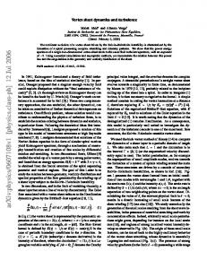
Laminar and turbulent water ow over the hull of a submarine Flow visualization of a turbulent jet, made by laser-induced uorescence. The jet exhibits a wide range of length scales, an important characteristic of turbulent ows.
ow regime characterized by chaotic property changes. This includes low momentum di usion, high momentum convection, and rapid variation of pressure and velocity in space and time. Flow in which the kinetic energy dies out due to the action of uid molecular viscosity is called laminar ow. While there is no theorem relating the non-dimensional Reynolds number (Re) to turbulence, ows at Reynolds numbers larger than 5000 are typically (but not necessarily) turbulent, while those at low Reynolds numbers usually remain laminar. In Poiseuille ow, for example, turbulence can rst be sustained if the Reynolds number Turbulence in the tip vortex from an airplane wing is larger than a critical value of about 2040;[1] moreover, the turbulence is generally interspersed with laminar ow until a larger Reynolds number of about 4000. sulting in a reduction of overall drag. Although laminarIn turbulent ow, unsteady vortices appear on many scales turbulent transition is not governed by Reynolds number, and interact with each other. Drag due to boundary layer the same transition occurs if the size of the object is gradskin friction increases. The structure and location of ually increased, or the viscosity of the uid is decreased, boundary layer separation often changes, sometimes re- or if the density of the uid is increased. Nobel Laure1
2
CHAPTER 1. TURBULENCE
ate Richard Feynman described turbulence as “the most turbulent di usivity concept assumes a constitutive relaimportant unsolved problem of classical physics.”[2] tion between a turbulent ux and the gradient of a mean variable similar to the relation between ux and gradient that exists for molecular transport. In the best case, this assumption is only an approximation. Nevertheless, the 1.1 Features turbulent di usivity is the simplest approach for quantitative analysis of turbulent ows, and many models have Turbulence is characterized by the following features: been postulated to calculate it. For instance, in large bodies of water like oceans this coe cient can be found using • Irregularity: Turbulent ows are always highly ir- Richardson's four-third power law and is governed by the regular. For this reason, turbulence problems are random walk principle. In rivers and large ocean currents, normally treated statistically rather than determinis- the di usion coe cient is given by variations of Elder’s tically. Turbulent ow is chaotic. However, not all formula. chaotic ows are turbulent. Turbulence causes the formation of eddies of many dif• Di usivity: The readily available supply of energy ferent length scales. Most of the kinetic energy of the turin turbulent ows tends to accelerate the homoge- bulent motion is contained in the large-scale structures. nization (mixing) of uid mixtures. The character- The energy “cascades” from these large-scale structures istic which is responsible for the enhanced mixing to smaller scale structures by an inertial and essentially and increased rates of mass, momentum and energy inviscid mechanism. This process continues, creating transports in a ow is called “di usivity”. smaller and smaller structures which produces a hierar• Rotationality: Turbulent ows have non-zero vor- chy of eddies. Eventually this process creates structures ticity and are characterized by a strong three- that are small enough that molecular di usion becomes dimensional vortex generation mechanism known as important and viscous dissipation of energy nally takes vortex stretching. In uid dynamics, they are essen- place. The scale at which this happens is the Kolmogorov tially vortices subjected to stretching associated with length scale. a corresponding increase of the component of vorticity in the stretching direction—due to the conservation of angular momentum. On the other hand, vortex stretching is the core mechanism on which the turbulence energy cascade relies to establish the structure function. In general, the stretching mechanism implies thinning of the vortices in the direction perpendicular to the stretching direction due to volume conservation of uid elements. As a result, the radial length scale of the vortices decreases and the larger ow structures break down into smaller structures. The process continues until the small scale structures are small enough that their kinetic energy can be transformed by the uid’s molecular viscosity into heat. This is why turbulence is always rotational and three dimensional. For example, atmospheric cyclones are rotational but their substantially two-dimensional shapes do not allow vortex generation and so are not turbulent. On the other hand, oceanic ows are dispersive but essentially non rotational and therefore are not turbulent.
• Dissipation: To sustain turbulent ow, a persistent source of energy supply is required because turbulence dissipates rapidly as the kinetic energy is converted into internal energy by viscous shear stress. Turbulent di usion is usually described by a turbulent di usion coe cient. This turbulent di usion coe cient is de ned in a phenomenological sense, by analogy with the molecular di usivities, but it does not have a true physical meaning, being dependent on the ow conditions, and not a property of the uid itself. In addition, the
Via this energy cascade, turbulent ow can be realized as a superposition of a spectrum of velocity uctuations and eddies upon a mean ow. The eddies are loosely dened as coherent patterns of velocity, vorticity and pressure. Turbulent ows may be viewed as made of an entire hierarchy of eddies over a wide range of length scales and the hierarchy can be described by the energy spectrum that measures the energy in velocity uctuations for each length scale (wavenumber). The scales in the energy cascade are generally uncontrollable and highly nonsymmetric. Nevertheless, based on these length scales these eddies can be divided into three categories. 1. Integral length scales: Largest scales in the energy spectrum. These eddies obtain energy from the mean ow and also from each other. Thus, these are the energy production eddies which contain most of the energy. They have the large velocity uctuation and are low in frequency. Integral scales are highly anisotropic and are de ned in terms of the normalized two-point velocity correlations. The maximum length of these scales is constrained by the characteristic length of the apparatus. For example, the largest integral length scale of pipe ow is equal to the pipe diameter. In the case of atmospheric turbulence, this length can reach up to the order of several hundreds kilometers. 2. Kolmogorov length scales: Smallest scales in the spectrum that form the viscous sub-layer range. In this range, the energy input from nonlinear interactions and the energy drain from viscous dissipation are in exact balance. The small scales have high
3
1.2. EXAMPLES OF TURBULENCE frequency, causing turbulence to be locally isotropic and homogeneous. 3. Taylor microscales: The intermediate scales between the largest and the smallest scales which make the inertial subrange. Taylor micro-scales are not dissipative scale but pass down the energy from the largest to the smallest without dissipation. Some literatures do not consider Taylor micro-scales as a characteristic length scale and consider the energy cascade to contain only the largest and smallest scales; while the latter accommodate both the inertial sub-range and the viscous-sub layer. Nevertheless, Taylor micro-scales are often used in describing the term “turbulence” more conveniently as these Taylor micro-scales play a dominant role in energy and momentum transfer in the wavenumber space. Although it is possible to nd some particular solutions of the Navier-Stokes equations governing uid motion, all such solutions are unstable to nite perturbations at large Reynolds numbers. Sensitive dependence on the initial and boundary conditions makes uid ow irregular both in time and in space so that a statistical description is needed. The Russian mathematician Andrey Kolmogorov proposed the rst statistical theory of turbulence, based on the aforementioned notion of the energy cascade (an idea originally introduced by Richardson) and the concept of self-similarity. As a result, the Kolmogorov microscales were named after him. It is now known that the self-similarity is broken so the statistical description is presently modi ed.[3] Still, a complete description of turbulence remains one of the unsolved problems in physics. According to an apocryphal story, Werner Heisenberg was asked what he would ask God, given the opportunity. His reply was: “When I meet God, I am going to ask him two questions: Why relativity? And why turbulence? I really believe he will have an answer for the rst.”[4] A similar witticism has been attributed to Horace Lamb (who had published a noted text book on Hydrodynamics)—his choice being quantum electrodynamics (instead of relativity) and turbulence. Lamb was quoted as saying in a speech to the British Association for the Advancement of Science, “I am an old man now, and when I die and go to heaven there are two matters on which I hope for enlightenment. One is quantum electrodynamics, and the other is the turbulent motion of uids. And about the former I am rather optimistic.”[5][6]
1.2 Examples of turbulence • Smoke rising from a cigarette is turbulent ow. For the rst few centimeters, the ow is certainly laminar. Then smoke becomes turbulent as its Reynolds number increases, as its velocity and characteristic length are both increasing. • Flow over a golf ball. (This can be best understood by considering the golf ball to be stationary, with air owing over it.) If the golf ball were smooth, the boundary layer ow over the front of the sphere would be laminar at typical conditions. However, the boundary layer would separate early, as the pressure gradient switched from favorable (pressure decreasing in the ow direction) to unfavorable (pressure increasing in the ow direction), creating a large region of low pressure behind the ball that creates high form drag. To prevent this from happening, the surface is dimpled to perturb the boundary layer and promote transition to turbulence. This results in higher skin friction, but moves the point of boundary layer separation further along, resulting in lower form drag and lower overall drag. • The mixing of warm and cold air in the atmosphere by wind, which causes clear-air turbulence experienced during airplane ight, as well as poor astronomical seeing (the blurring of images seen through the atmosphere.) • Most of the terrestrial atmospheric circulation • The oceanic and atmospheric mixed layers and intense oceanic currents. • The ow conditions in many industrial equipment (such as pipes, ducts, precipitators, gas scrubbers, dynamic scraped surface heat exchangers, etc.) and machines (for instance, internal combustion engines and gas turbines). • The external ow over all kind of vehicles such as cars, airplanes, ships and submarines. • The motions of matter in stellar atmospheres. • A jet exhausting from a nozzle into a quiescent uid. As the ow emerges into this external uid, shear layers originating at the lips of the nozzle are created. These layers separate the fast moving jet from the external uid, and at a certain critical Reynolds number they become unstable and break down to turbulence.
A more detailed presentation of turbulence with emphasis on high-Reynolds number ow, intended for a general readership of physicists and applied mathematicians, is found in the Scholarpedia articles by R. Benzi and U. Frisch[7] and by G. Falkovich.[8]
• Snow fences work by inducing turbulence in the wind, forcing it to drop much of its snow load near the fence.
There are many scales of meteorological motions; in this context turbulence a ects small-scale motions.[9]
• Bridge supports (piers) in water. In the late summer and fall, when river ow is slow, water ows
4
CHAPTER 1. TURBULENCE
smoothly around the support legs. In the spring, given time are when the ow is faster, a higher Reynolds Number ∂T q = v ′ y ρcP T ′ = −kturb is associated with the ow. The ow may start o ∂y | {z } laminar but is quickly separated from the leg and value experimental becomes turbulent. ∂vx τ = −ρv ′ y v ′ x = µturb ∂y | {z } • In many geophysical ows (rivers, atmospheric value experimental boundary layer), the ow turbulence is dominated by the coherent structure activities and associated where cP is the heat capacity at constant pressure, ρ is turbulent events. A turbulent event is a series of tur- the density of the uid, µturb is the coe cient of turbulent bulent uctuations that contain more energy than the viscosity and kturb is the turbulent thermal conductivity. average ow turbulence.[10][11] The turbulent events [12] are associated with coherent ow structures such as eddies and turbulent bursting, and they play a critical role in terms of sediment scour, accretion and 1.4 Kolmogorov’s theory of 1941 transport in rivers as well as contaminant mixing and dispersion in rivers and estuaries, and in the atmoRichardson’s notion of turbulence was that a turbulent sphere. ow is composed by “eddies” of di erent sizes. The sizes • In the medical eld of cardiology, a stethoscope is de ne a characteristic length scale for the eddies, which used to detect heart sounds and bruits, which are are also characterized by velocity scales and time scales due to turbulent blood ow. In normal individuals, (turnover time) dependent on the length scale. The large heart sounds are a product of turbulent ow as heart eddies are unstable and eventually break up originating valves close. However, in some conditions turbu- smaller eddies, and the kinetic energy of the initial large lent ow can be audible due to other reasons, some eddy is divided into the smaller eddies that stemmed from of them pathological. For example, in advanced it. These smaller eddies undergo the same process, givatherosclerosis, bruits (and therefore turbulent ow) ing rise to even smaller eddies which inherit the energy can be heard in some vessels that have been nar- of their predecessor eddy, and so on. In this way, the enrowed by the disease process. ergy is passed down from the large scales of the motion to smaller scales until reaching a su ciently small length scale such that the viscosity of the uid can e ectively 1.3 Heat and momentum transfer dissipate the kinetic energy into internal energy. In his original theory of 1941, Kolmogorov postulated that for very high Reynolds numbers, the small scale turbulent motions are statistically isotropic (i.e. no preferential spatial direction could be discerned). In general, the large scales of a ow are not isotropic, since they are determined by the particular geometrical features of Assume for a two-dimensional turbulent ow that one was the boundaries (the size characterizing the large scales able to locate a speci c point in the uid and measure the will be denoted as L). Kolmogorov’s idea was that in the actual velocity v = (vx , vy ) of every particle that passed Richardson’s energy cascade this geometrical and directhrough that point at any given time. Then one would nd tional information is lost, while the scale is reduced, so the actual velocity uctuating about a mean value: that the statistics of the small scales has a universal charvx = vx + v ′ x ,vy = vy + v ′ y acter: they are the same for all turbulent ows when the |{z} |{z} Reynolds number is su ciently high. mean uctuation
When ow is turbulent, particles exhibit additional transverse motion which enhances the rate of energy and momentum exchange between them thus increasing the heat transfer and the friction coe cient.
value
) ( and similarly for temperature T = T + T ′ and pres( ) sure P = P + P ′ , where the primed quantities denote uctuations superposed to the mean. This decomposition of a ow variable into a mean value and a turbulent uctuation was originally proposed by Osborne Reynolds in 1895, and is considered to be the beginning of the systematic mathematical analysis of turbulent ow, as a subeld of uid dynamics. While the mean values are taken as predictable variables determined by dynamics laws, the turbulent uctuations are regarded as stochastic variables.
Thus, Kolmogorov introduced a second hypothesis: for very high Reynolds numbers the statistics of small scales are universally and uniquely determined by the viscosity ( ν ) and the rate of energy dissipation ( ε ). With only these two parameters, the unique length that can be formed by dimensional analysis is
η=
(
ν3 ε
)1/4
The heat ux and momentum transfer (represented by the This is today known as the Kolmogorov length scale (see shear stress τ ) in the direction normal to the ow for a Kolmogorov microscales).
5
1.4. KOLMOGOROV’S THEORY OF 1941 A turbulent ow is characterized by a hierarchy of scales through which the energy cascade takes place. Dissipation of kinetic energy takes place at scales of the order of Kolmogorov length η , while the input of energy into the cascade comes from the decay of the large scales, of order L. These two scales at the extremes of the cascade can di er by several orders of magnitude at high Reynolds numbers. In between there is a range of scales (each one with its own characteristic length r) that has formed at the expense of the energy of the large ones. These scales are very large compared with the Kolmogorov length, but still very small compared with the large scale of the ow (i.e. η ≪ r ≪ L ). Since eddies in this range are much larger than the dissipative eddies that exist at Kolmogorov scales, kinetic energy is essentially not dissipated in this range, and it is merely transferred to smaller scales until viscous e ects become important as the order of the Kolmogorov scale is approached. Within this range inertial e ects are still much larger than viscous e ects, and it is possible to assume that viscosity does not play a role in their internal dynamics (for this reason this range is called “inertial range”).
considerable experimental evidence has accumulated that supports it.[13] In spite of this success, Kolmogorov theory is at present under revision. This theory implicitly assumes that the turbulence is statistically self-similar at di erent scales. This essentially means that the statistics are scaleinvariant in the inertial range. A usual way of studying turbulent velocity elds is by means of velocity increments: δu(r) = u(x + r) − u(x) that is, the di erence in velocity between points separated by a vector r (since the turbulence is assumed isotropic, the velocity increment depends only on the modulus of r). Velocity increments are useful because they emphasize the e ects of scales of the order of the separation r when statistics are computed. The statistical scale-invariance implies that the scaling of velocity increments should occur with a unique scaling exponent β , so that when r is scaled by a factor λ ,
Hence, a third hypothesis of Kolmogorov was that at very high Reynolds number the statistics of scales in the range η ≪ r ≪ L are universally and uniquely determined by δu(λr) the scale r and the rate of energy dissipation ε . The way in which the kinetic energy is distributed over the multiplicity of scales is a fundamental characterization of a turbulent ow. For homogeneous turbulence (i.e., statistically invariant under translations of the reference frame) this is usually done by means of the energy spectrum function E(k) , where k is the modulus of the wavevector corresponding to some harmonics in a Fourier representation of the ow velocity eld u(x):
u(x) =
∫∫∫
R3
b(k)eik·x d3 k u
should have the same statistical distribution as λβ δu(r) with β independent of the scale r. From this fact, and other results of Kolmogorov 1941 theory, it follows that the statistical moments of the velocity increments (known as structure functions in turbulence) should scale as ⟨[δu(r)]n ⟩ = Cn εn/3 rn/3
where û(k) is the Fourier transform of the velocity eld. Thus, E(k)dk represents the contribution to the kinetic where the brackets denote the statistical average, and the energy from all the Fourier modes with k < |k| < k + dk, Cn would be universal constants. and therefore, There is considerable evidence that turbulent ows deviate from this behavior. The scaling exponents deviate from the n/3 value predicted by the theory, becoming a ∫ ∞ 1 non-linear function of the order n of the structure funcE(k)dk ⟨ui ui ⟩ = 2 0 tion. The universality of the constants have also been where 1/2⟨ui ui ⟩ is the mean turbulent kinetic energy questioned. For low orders the discrepancy with the Kolof the ow. The wavenumber k corresponding to length mogorov n/3 value is very small, which explain the sucscale r is k = 2π/r . Therefore, by dimensional analysis, cess of Kolmogorov theory in regards to low order statisthe only possible form for the energy spectrum function tical moments. In particular, it can be shown that when the energy spectrum follows a power law according with the third Kolmogorov’s hypothesis is E(k) = Cε2/3 k −5/3
E(k) ∝ k −p
where C would be a universal constant. This is one of with 1 < p < 3 , the second order structure function has the most famous results of Kolmogorov 1941 theory, and also a power law, with the form
6
CHAPTER 1. TURBULENCE • Vortex generator
⟨[δu(r)]2 ⟩ ∝ rp−1 Since the experimental values obtained for the second order structure function only deviate slightly from the 2/3 value predicted by Kolmogorov theory, the value for p is very near to 5/3 (di erences are about 2%[14] ). Thus the “Kolmogorov −5/3 spectrum” is generally observed in turbulence. However, for high order structure functions the di erence with the Kolmogorov scaling is significant, and the breakdown of the statistical self-similarity is clear. This behavior, and the lack of universality of the Cn constants, are related with the phenomenon of intermittency in turbulence. This is an important area of research in this eld, and a major goal of the modern theory of turbulence is to understand what is really universal in the inertial range.
1.5
See also
• Astronomical seeing • Atmospheric dispersion modeling • Chaos theory • Clear-air turbulence • Constructal theory • Downdrafts
• Wake turbulence • Wave turbulence • Wingtip vortices • Wind tunnel
• Di erent types of boundary conditions in uid dynamics
1.6 References and notes [1] Avila, K.; D. Moxey; A. de Lozar; M. Avila; D. Barkley; B. Hof (July 2011). “The OnScience 333 set of Turbulence in Pipe Flow”. Bibcode:2011Sci...333..192A. (6039): 192–196. doi:10.1126/science.1203223. [2] “Turbulence theory gets a bit choppy”. September 10, 2006.
USA Today.
[3] weizmann.ac.il [4] MARSHAK, ALEX (2005). 3D radiative transfer in cloudy atmospheres; pg.76. Springer. ISBN 978-3-54023958-1. [5] Mullin, Tom (11 November 1989). “Turbulent times for uids”. New Scientist. [6] Davidson, P. A. (2004). Turbulence: An Introduction for Scientists and Engineers. Oxford University Press. ISBN 978-0-19-852949-1.
• Eddy covariance
[7] scholarpedia.org; R. Benzi and U. Frisch, Scholarpedia, “Turbulence”.
• Fluid dynamics
[8] scholarpedia.org; G. Falkovich, Scholarpedia, “Cascade and scaling”.
• Darcy–Weisbach equation • Eddy
• Navier-Stokes equations • Large eddy simulation • Poiseuille’s law
• Lagrangian coherent structure • Turbulence kinetic energy • Mesocyclones • Navier-Stokes existence and smoothness • Reynolds Number • Swing bowling • Taylor microscale • Turbulence modeling • Velocimetry • Vortex
[9] Stull, Roland B. (1994). An Introduction to Boundary Layer Meteorology (1st ed., repr. ed.). Dordrecht [u.a.]: Kluwer. p. 20. ISBN 978-90-277-2769-5. [10] Narasimha R, Rudra Kumar S, Prabhu A, Kailas SV (2007). “Turbulent ux events in a nearly neutral atmospheric boundary layer”. Philosophical Transactions of the Royal Society A: Mathematical, Physical and Engineering Sciences (Phil Trans R Soc Ser A, Vol. 365, pp. 841–858) 365 (1852): 841–858. Bibcode:2007RSPTA.365..841N. doi:10.1098/rsta.2006.1949. [11] Trevethan M, Chanson H (2010). “Turbulence and Turbulent Flux Events in a Small Estuary”. Environmental Fluid Mechanics (Environmental Fluid Mechanics, Vol. 10, pp. 345-368) 10 (3): 345–368. doi:10.1007/s10652009-9134-7. [12] H. Tennekes and J. L. Lumley, “A First Course in Turbulence”, The MIT Press, (1972). [13] U. Frisch. Turbulence: The Legacy of A. N. Kolmogorov. Cambridge University Press, 1995. [14] J. Mathieu and J. Scott An Introduction to Turbulent Flow. Cambridge University Press, 2000.
7
1.8. EXTERNAL LINKS
1.7
Further reading
1.7.1 General
1.8 External links • Center for Turbulence Research, Stanford University
• G Falkovich and K.R. Sreenivasan. Lessons from hydrodynamic turbulence, Physics Today, vol. 59, no. 4, pages 43–49 (April 2006).
• Scienti c American article
• U. Frisch. Turbulence: The Legacy of A. N. Kolmogorov. Cambridge University Press, 1995.
• international CFD database iCFDdatabase
• P. A. Davidson. Turbulence - An Introduction for Scientists and Engineers. Oxford University Press, 2004.
• Fluid Mechanics website with movies, Q&A, etc
• J. Cardy, G. Falkovich and K. Gawedzki (2008) Non-equilibrium statistical mechanics and turbulence. Cambridge University Press • P. A. Durbin and B. A. Pettersson Reif. Statistical Theory and Modeling for Turbulent Flows. Johns Wiley & Sons, 2001. • T. Bohr, M.H. Jensen, G. Paladin and A.Vulpiani. Dynamical Systems Approach to Turbulence, Cambridge University Press, 1998. • J. M. McDonough (2007). Introductory Lectures on Turbulence - Physics, Mathematics, and Modeling
1.7.2 Original scienti c research papers and classic monographs • Kolmogorov, Andrey Nikolaevich (1941). “The local structure of turbulence in incompressible viscous uid for very large Reynolds numbers”. Proceedings of the USSR Academy of Sciences (in Russian) 30: 299–303., translated into English by V. Levin: Kolmogorov, Andrey Nikolaevich (July 8, 1991). “The local structure of turbulence in incompressible viscous uid for very large Reynolds numbers”. Proceedings of the Royal Society A 434 (1991): 9–13. Bibcode:1991RSPSA.434....9K. doi:10.1098/rspa.1991.0075. • Kolmogorov, Andrey Nikolaevich (1941). “Dissipation of Energy in the Locally Isotropic Turbulence”. Proceedings of the USSR Academy of Sciences (in Russian) 32: 16–18., translated into English by Kolmogorov, Andrey Nikolaevich (July 8, 1991). “The local structure of turbulence in incompressible viscous uid for very large Reynolds numbers”. Proceedings of the Royal Society A 434 (1980): 15–17. Bibcode:1991RSPSA.434...15K. doi:10.1098/rspa.1991.0076. • G. K. Batchelor, The theory of homogeneous turbulence. Cambridge University Press, 1953.
• Air Turbulence Forecast • Turbulent ow in a pipe on YouTube • Johns Hopkins public database with direct numerical simulation data
Chapter 2
Turbulence modeling Turbulence modeling is the construction and use of a model to predict the e ects of turbulence. Averaging is often used to simplify the solution of the governing equations of turbulence, but models are needed to represent scales of the ow that are not resolved.[1]
In this model, the additional turbulence stresses are given by augmenting the molecular viscosity with an eddy viscosity.[3] This can be a simple constant eddy viscosity (which works well for some free shear ows such as axisymmetric jets, 2-D jets, and mixing layers).
2.1
2.3 Prandtl’s mixing-length concept
Closure problem
A closure problem arises in the Reynolds-averaged Navier-Stokes (RANS) equation because of the non- Later, Ludwig Prandtl introduced the additional concept linear term −ρυi′ υj′ from the convective acceleration, of the mixing length, along with the idea of a boundary known as the Reynolds stress, layer. For wall-bounded turbulent ows, the eddy viscosity must vary with distance from the wall, hence the addition of the concept of a 'mixing length'. In the simplest Rij = −ρυi′ υj′ [2] wall-bounded ow model, the eddy viscosity is given by the equation: Closing the RANS equation requires modeling the Reynold’s stress Rij . ∂u 2 νt = lm ∂y
2.2
Eddy viscosity
where:
∂u ∂y lm
Joseph Boussinesq was the rst practitioner of this (i.e. modeling the Reynold’s stress), introducing the concept of eddy viscosity. In 1887 Boussinesq proposed relating the turbulence stresses to the mean ow to close the system of equations. Here the Boussinesq hypothesis is applied to model the Reynolds stress term. Note that a new proportionality constant νt > 0 , the turbulence eddy viscosity, has been introduced. Models of this type are known as eddy viscosity models or EVM’s. −υi′ υj′ = νt
(
∂υ ¯i ∂xj
+
∂υ ¯j ∂xi
)
This simple model is the basis for the "law of the wall", which is a surprisingly accurate model for wall-bounded, attached (not separated) ow elds with small pressure gradients. More general turbulence models have evolved over time, with most modern turbulence models given by eld equations similar to the Navier-Stokes equations.
− 32 Kδij
Which can be written in shorthand as
2.4 Smagorinsky model for the sub-grid scale eddy viscosity
−υi′ υj′ = 2νt Sij − 32 Kδij
where Sij is the mean rate of strain tensor
Among many others , Joseph Smagorinsky (1964) proposed a useful formula for the eddy viscosity in numerical models, based on the local derivatives of the velocity eld and the local grid size:
νt is the turbulence eddy viscosity K = 21 υi′ υi′ is the turbulence kinetic energy and δij is the Kronecker delta. 8
9
2.7. REFERENCES
νt = ∆x∆y
2.5
√(
∂u ∂x
)2
+
(
∂v ∂y
)2
1 + 2
(
∂u ∂v + ∂y ∂x
)2
Spalart–Allmaras, k–ε and k– ω models
The Boussinesq hypothesis is employed in the Spalart– Allmaras (S–A), k–ε (k–epsilon), and k–ω (k–omega) models and o ers a relatively low cost computation for the turbulence viscosity νt . The S–A model uses only one additional equation to model turbulence viscosity transport, while the k models use two.
2.6
Common models
The following is a list of commonly employed models in modern engineering applications. • Spalart–Allmaras (S–A) • k–ε (k–epsilon) • k–ω (k–omega) • SST (Menter’s Shear Stress Transport) • Reynolds stress equation model
2.7
References
2.7.1 Notes [1] Ching Jen Chen, Shenq-Yuh Jaw (1998), Fundamentals of turbulence modeling, Taylor & Francis [2] Andersson, Bengt et al (2012). Computational uid dynamics for engineers. Cambridge: Cambridge University Press. p. 83. ISBN 978-1-107-01895-2. [3] John J. Bertin, Jacques Periaux, Josef Ballmann, Advances in Hypersonics: Modeling hypersonic ows
2.7.2 Other • Townsend, A.A. (1980) “The Structure of Turbulent Shear Flow” 2nd Edition (Cambridge Monographs on Mechanics) • Bradshaw, P. (1971) “An introduction to turbulence and its measurement” (Pergamon Press) • Wilcox C. D., (1998), “Turbulence Modeling for CFD” 2nd Ed., (DCW Industries, La Cañada)
Chapter 3
Reynolds stress equation model Reynolds stress equation model (RSM), also known as second order or second moment closure model is the most complex classical turbulence model. Several shortcomings of k-epsilon turbulence model were observed when it was attempted to predict ows with complex strain elds or substantial body forces. Under those conditions the individual Reynolds stresses were not found to be accurate while using formula ( ) ∂Ui 2 2 i −ρu′i u′j = µt ∂U ∂xj + ∂xi − 3 ρkδij = 2µtEij − 3 ρkδij
of normal Reynolds stresses and decreases Reynolds shear stresses. A comprehensive model that takes into account these e ects was given by Launder and Rodi (1975).
3.3 Dissipation term
The modelling of dissipation rate ϵij assumes that the small dissipative eddies are isotropic. This term a ects The equation for the transport of kinematic Reynolds only the normal Reynolds stresses. [2] stress Rij = u′i u′j = −τij /ρ is [1] ϵij = 2/3ϵδij DRij Dt = Dij + Pij + Πij + Ωij − εij where ϵ is dissipation rate of turbulent kinetic energy, and Rate of change of Rij + Transport of Rij by convection δij = 1 when i = j and 0 when i ≠ j = Transport of Rij by di usion + Rate of production of Rij + Transport of Rij due to turbulent pressure-strain interactions + Transport of Rij due to rotation + Rate of 3.4 Di usion term dissipation of Rij . The six partial di erential equations above represent six The modelling of di usion term Dij is based on the asindependent Reynolds stresses. The models that we need sumption that the rate of transport of Reynolds stresses to solve the above equation are derived from the work of by di usion is proportional to the gradients of Reynolds Launder, Rodi and Reece (1975). stresses. The simplest form of Dij that is followed by commercial CFD codes is ) ( ) ( ∂Rij Dij = ∂x∂m σvkt ∂xm = div σvkt ∇(Rij )
3.1
Production term
2
The Production term that is used in CFD computations with Reynolds stress transport equations is ) ( ∂U ∂Ui Pij = − Rim ∂xmj + Rjm ∂x m
3.2
Pressure-strain interactions
Pressure-strain interactions a ect the Reynolds stresses by two di erent physical processes: pressure uctuations due to eddies interacting with one another and pressure uctuation of an eddy with a region of di erent mean velocity. This redistributes energy among normal Reynolds stresses and thus makes them more isotropic. It also reduces the Reynolds shear stresses. It is observed that the wall e ect increases the anisotropy
where υt = Cµ kϵ , σk = 1.0 and Cµ = 0.9
3.5 Pressure-strain term
correlation
The pressure-strain correlation term promotes isotropy of the turbulence by redistributing energy amongst the normal Reynolds stresses.The pressure-strain interactions is the most important term to model correctly. Their e ect on Reynolds stresses is caused by pressure uctuations due to interaction of eddies with each other and pressure uctuations due to interaction of an eddy with region of ow having di erent mean velocity. The correction term is given as [3] ( ( ) ) Πij = −C1 kϵ Rij − 23 kδij − C2 Pij − 32 P δij
10
11
3.11. REFERENCES
3.6
Rotational term
The rotational term is given as [4] Ωij = −2ωk (Rjm eikm + Rim ejkm )
3.11 References [1] Bengt Andersson , Ronnie Andersson s (2012). Computational Fluid Dynamics for Engineers (First ed.). Cambridge University Press, New York. p. 97. ISBN 9781107018952.
here ωk is the rotation vector, eijk =1 if i,j,k are in cyclic order and are di erent, eijk =−1 if i,j,k are in anti-cyclic order and are di erent and eijk =0 in case any two indices are same.
[2] Peter S. Bernard & James M. Wallace (2002). Turbulent Flow: Analysis, Measurement & Prediction. John Wiley & Sons. p. 324. ISBN 0471332194.
3.7
[3] Magnus Hallback (1996). Turbulence and Transition Modelling (First ed.). Kluwer Academic Publishers. p. 117. ISBN 0792340604.
Advantages of RSM
1)Compared with k-ε model, it is simple because of the use of an isotropic eddy viscosity. 2)It is the most general of all turbulence models and work reasonably well for a large number of engineering ows. 3)It requires only the initial and/or boundary conditions to be supplied. 4)Since the production terms need not be modelled, it can selectively damp the stresses due to buoyancy, curvature e ects etc.
3.8
Disadvantages of RSM
1)It requires very large computing costs. 2)It is not very widely validated as the k-ε model and mixing length models. 3)Due to identical problems with the ε-equation modelling, it performs just as poorly as the k-ε model in some problems. 4)Because of being isotropic, it is not good in predicting normal stresses and is unable to account for irrotational strains.
3.9
See also
• Reynolds Stress • Isotropy • Turbulence Modeling • Eddy • k-epsilon turbulence model
3.10
See also
• k-epsilon turbulence model • Mixing length model
[4] H.Versteeg & W.Malalasekera (2013). An Introduction to Computational Fluid Dynamics (Second ed.). Pearson Education Limited. p. 96. ISBN 9788131720486.
3.12 Bibliography • “An Introduction to Computational Fluid Dynamics”,Second Edition by Versteeg & Malalasekera, published by Pearson Education Limited. • “Turbulence : An Introduction for Scientists and Engineers” By P.A. Davidson. • “Turbulence Models & Their Applications” By Tuncer Cebeci, published by Horizons Publications Inc.
Chapter 4
Boundary layer For the anatomical structure, see Boundary layer of uterus. In physics and uid mechanics, a boundary layer is the
u0
u(y)
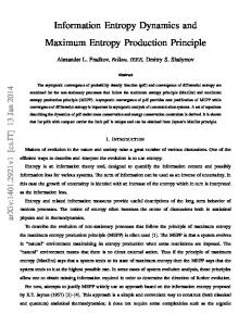
Laminar boundary layer velocity pro le
Boundary layer visualization, showing transition from laminar to turbulent condition
layer of uid in the immediate vicinity of a bounding surface where the e ects of viscosity are signi cant. In the Earth’s atmosphere, the atmospheric boundary layer is the air layer near the ground a ected by diurnal heat, moisture or momentum transfer to or from the surface. On an aircraft wing the boundary layer is the part of the ow close to the wing, where viscous forces distort the surrounding non-viscous ow. See Reynolds number. Laminar boundary layers can be loosely classi ed according to their structure and the circumstances under which they are created. The thin shear layer which develops on an oscillating body is an example of a Stokes boundary layer, while the Blasius boundary layer refers to the wellknown similarity solution near an attached at plate held in an oncoming unidirectional ow. When a uid rotates and viscous forces are balanced by the Coriolis e ect (rather than convective inertia), an Ekman layer forms. In the theory of heat transfer, a thermal boundary layer occurs. A surface can have multiple types of boundary layer simultaneously.
4.1
Aerodynamics
The aerodynamic boundary layer was rst de ned by Ludwig Prandtl in a paper presented on August 12, 1904 at the third International Congress of Mathematicians in Heidelberg, Germany. It simpli es the equations of uid ow by dividing the ow eld into two areas: one in-
side the boundary layer, dominated by viscosity and creating the majority of drag experienced by the boundary body; and one outside the boundary layer, where viscosity can be neglected without signi cant e ects on the solution. This allows a closed-form solution for the ow in both areas, a signi cant simpli cation of the full Navier– Stokes equations. The majority of the heat transfer to and from a body also takes place within the boundary layer, again allowing the equations to be simpli ed in the ow eld outside the boundary layer. The pressure distribution throughout the boundary layer in the direction normal to the surface (such as an airfoil) remains constant throughout the boundary layer, and is the same as on the surface itself. The thickness of the velocity boundary layer is normally de ned as the distance from the solid body at which the viscous ow velocity is 99% of the freestream velocity (the surface velocity of an inviscid ow). Displacement Thickness is an alternative de nition stating that the boundary layer represents a de cit in mass ow compared to inviscid ow with slip at the wall. It is the distance by which the wall would have to be displaced in the inviscid case to give the same total mass ow as the viscous case. The no-slip condition requires the ow velocity at the surface of a solid object be zero and the uid temperature be equal to the temperature of the surface. The ow velocity will then increase rapidly within the boundary layer, governed by the boundary layer equations, below. The thermal boundary layer thickness is similarly the distance from the body at which the temperature is 99% of the temperature found from an inviscid solution. The ratio of the two thicknesses is governed by the Prandtl number. If the Prandtl number is 1, the two boundary layers
12
13
4.2. NAVAL ARCHITECTURE
are the same thickness. If the Prandtl number is greater sometimes used to reduce or eliminate the e ect of the than 1, the thermal boundary layer is thinner than the ve- boundary layer. locity boundary layer. If the Prandtl number is less than 1, which is the case for air at standard conditions, the thermal boundary layer is thicker than the velocity boundary 4.2 Naval architecture layer. In high-performance designs, such as gliders and commercial aircraft, much attention is paid to controlling the behavior of the boundary layer to minimize drag. Two e ects have to be considered. First, the boundary layer adds to the e ective thickness of the body, through the displacement thickness, hence increasing the pressure drag. Secondly, the shear forces at the surface of the wing create skin friction drag. At high Reynolds numbers, typical of full-sized aircraft, it is desirable to have a laminar boundary layer. This results in a lower skin friction due to the characteristic velocity pro le of laminar ow. However, the boundary layer inevitably thickens and becomes less stable as the ow develops along the body, and eventually becomes turbulent, the process known as boundary layer transition. One way of dealing with this problem is to suck the boundary layer away through a porous surface (see Boundary layer suction). This can reduce drag, but is usually impractical due to its mechanical complexity and the power required to move the air and dispose of it. Natural laminar ow techniques push the boundary layer transition aft by reshaping the aerofoil or fuselage so that its thickest point is more aft and less thick. This reduces the velocities in the leading part and the same Reynolds number is achieved with a greater length. At lower Reynolds numbers, such as those seen with model aircraft, it is relatively easy to maintain laminar ow. This gives low skin friction, which is desirable. However, the same velocity pro le which gives the laminar boundary layer its low skin friction also causes it to be badly a ected by adverse pressure gradients. As the pressure begins to recover over the rear part of the wing chord, a laminar boundary layer will tend to separate from the surface. Such ow separation causes a large increase in the pressure drag, since it greatly increases the e ective size of the wing section. In these cases, it can be advantageous to deliberately trip the boundary layer into turbulence at a point prior to the location of laminar separation, using a turbulator. The fuller velocity pro le of the turbulent boundary layer allows it to sustain the adverse pressure gradient without separating. Thus, although the skin friction is increased, overall drag is decreased. This is the principle behind the dimpling on golf balls, as well as vortex generators on aircraft. Special wing sections have also been designed which tailor the pressure recovery so laminar separation is reduced or even eliminated. This represents an optimum compromise between the pressure drag from ow separation and skin friction from induced turbulence.
Many of the principles that apply to aircraft also apply to ships, submarines, and o shore platforms. For ships, unlike aircraft, one deals with incompressible ows, where change in water density is negligible (a pressure rise close to 1000kPa leads to a change of only 2– 3 kg/m3 ). This eld of uid dynamics is called hydrodynamics. A ship engineer designs for hydrodynamics rst, and for strength only later. The boundary layer development, breakdown, and separation become critical because the high viscosity of water produces high shear stresses. Another consequence of high viscosity is the slip stream e ect, in which the ship moves like a spear tearing through a sponge at high velocity.
4.3 Boundary layer equations The deduction of the boundary layer equations was one of the most important advances in uid dynamics (Anderson, 2005). Using an order of magnitude analysis, the well-known governing Navier–Stokes equations of viscous uid ow can be greatly simpli ed within the boundary layer. Notably, the characteristic of the partial di erential equations (PDE) becomes parabolic, rather than the elliptical form of the full Navier–Stokes equations. This greatly simpli es the solution of the equations. By making the boundary layer approximation, the ow is divided into an inviscid portion (which is easy to solve by a number of methods) and the boundary layer, which is governed by an easier to solve PDE. The continuity and Navier–Stokes equations for a two-dimensional steady incompressible ow in Cartesian coordinates are given by ∂u ∂υ + =0 ∂x ∂y u
∂u 1 ∂p ∂u +υ =− +ν ∂x ∂y ρ ∂x
u
∂υ 1 ∂p ∂υ +υ =− +ν ∂x ∂y ρ ∂y
(
(
∂2u ∂2u + 2 ∂x2 ∂y ∂2υ ∂2υ + 2 ∂x2 ∂y
)
)
where u and υ are the velocity components, ρ is the density, p is the pressure, and ν is the kinematic viscosity of the uid at a point.
The approximation states that, for a su ciently high Reynolds number the ow over a surface can be divided into an outer region of inviscid ow una ected by visWhen using half-models in wind tunnels, a peniche is cosity (the majority of the ow), and a region close to the surface where viscosity is important (the boundary layer).
14
CHAPTER 4. BOUNDARY LAYER
Let u and υ be streamwise and transverse (wall normal) 4.4 Turbulent boundary layers velocities respectively inside the boundary layer. Using scale analysis, it can be shown that the above equations The treatment of turbulent boundary layers is far more of motion reduce within the boundary layer to become di cult due to the time-dependent variation of the ow properties. One of the most widely used techniques in which turbulent ows are tackled is to apply Reynolds ∂u ∂υ + =0 decomposition. Here the instantaneous ow properties ∂x ∂y are decomposed into a mean and uctuating component. Applying this technique to the boundary layer equations ∂u 1 ∂p ∂2u ∂u +υ =− +ν 2 u gives the full turbulent boundary layer equations not often ∂x ∂y ρ ∂x ∂y and if the uid is incompressible (as liquids are under given in literature: standard conditions): 1 ∂p =0 ρ ∂y
∂u ∂v + =0 ∂x ∂y
( 2 ) 1 ∂p ∂ u ∂2u ∂ ∂u ∂u ∂ =− +ν + − (u′ v ′ )− (u′2 ) The asymptotic analysis also shows that υ , the wall nor- u +v 2 2 ∂x ∂y ρ ∂x ∂x ∂y ∂y ∂x mal velocity, is small compared with u the streamwise ) ( 2 velocity, and that variations in properties in the stream∂ ′ ′ ∂2v 1 ∂p ∂ v ∂v ∂v ∂ ′2 wise direction are generally much lower than those in the u ∂x +v ∂y = − ρ ∂y +ν ∂x2 + ∂y 2 − ∂x (u v )− ∂y (v ) wall normal direction. Using the same order-of-magnitude analysis as for the Since the static pressure p is independent of y , then pres- instantaneous equations, these turbulent boundary layer sure at the edge of the boundary layer is the pressure equations generally reduce to become in their classical throughout the boundary layer at a given streamwise po- form: sition. The external pressure may be obtained through an application of Bernoulli’s equation. Let u0 be the uid velocity outside the boundary layer, where u and u0 are ∂u ∂v both parallel. This gives upon substituting for p the fol- ∂x + ∂y = 0 lowing result ∂ ′ ′ ∂u ∂u 1 ∂p ∂2u +v =− +ν 2 − (u v ) u ∂x ∂y ρ ∂x ∂y ∂y 2 ∂u0 ∂u ∂u ∂ u +υ = u0 +ν 2 u ∂p ∂x ∂y ∂x ∂y =0 ∂y with the boundary condition The additional term u′ v ′ in the turbulent boundary layer equations is known as the Reynolds shear stress and is ∂u ∂v unknown a priori. The solution of the turbulent bound+ =0 ∂x ∂y ary layer equations therefore necessitates the use of a For a ow in which the static pressure p also does not turbulence model, which aims to express the Reynolds shear stress in terms of known ow variables or derivachange in the direction of the ow then tives. The lack of accuracy and generality of such models is a major obstacle in the successful prediction of turbu∂p lent ow properties in modern uid dynamics. =0 ∂x A laminar sub-layer exists in the turbulent zone; it occurs so u0 remains constant. due to those uid molecules which are still in the very proximity of the surface, where the shear stress is maxiTherefore, the equation of motion simpli es to become mum and the velocity of uid molecules is zero. u
∂u ∂u ∂2u +υ =ν 2 ∂x ∂y ∂y
These approximations are used in a variety of practical ow problems of scienti c and engineering interest. The above analysis is for any instantaneous laminar or turbulent boundary layer, but is used mainly in laminar ow studies since the mean ow is also the instantaneous ow because there are no velocity uctuations present.
4.5 Heat and mass transfer In 1928, the French engineer André Lévêque observed that convective heat transfer in a owing uid is a ected only by the velocity values very close to the surface.[1][2] For ows of large Prandtl number, the temperature/mass transition from surface to freestream temperature takes
15
4.6. CONVECTIVE TRANSFER CONSTANTS FROM BOUNDARY LAYER ANALYSIS place across a very thin region close to the surface. Therefore, the most important uid velocities are those inside this very thin region in which the change in velocity can be considered linear with normal distance from the surface. In this way, for [
u(y) = u0 1 −
(y − h) h2
when y → 0 , then u(y) ≈ 2u0
] 2
y[ y] = u0 2− , h h
velocity v∞ ; x is position along the semi-in nite plate, and Re is the Reynolds Number given by ρv∞ x/µ ( ρ = density and µ = dynamic viscosity). The Blasius solution uses boundary conditions in a dimensionless form: vx −vS v∞ −vS vx −vS v∞ −vS
vy v∞
= 0 at y = 0
=
vx v∞
=
=
vx v∞
= 1 at y = ∞ and x = 0
y = θy h
where θ is the tangent of the Poiseuille parabola intersecting the wall. Although Lévêque’s solution was speci c to heat transfer into a Poiseuille ow, his insight helped lead other scientists to an exact solution of the thermal boundary-layer problem.[3] Schuh observed that in a boundary-layer, u is again a linear function of y, but that in this case, the wall tangent is a function of x.[4] He expressed this with a modi ed version of Lévêque’s prole,
u(y) = θ(x)y This results in a very good approximation, even for low P r numbers, so that only liquid metals with P r much less than 1 cannot be treated this way.[3] In 1962, Kestin and Persen published a paper describing solutions for heat transfer when the thermal boundary layer is contained entirely within the momentum layer and for various wall temperature distributions.[5] For the problem of a at plate with a temperature jump at x = x0 , they propose a substitution that reduces the parabolic thermal boundarylayer equation to an ordinary di erential equation. The solution to this equation, the temperature at any point in the uid, can be expressed as an incomplete gamma function.[2] Schlichting proposed an equivalent substitution that reduces the thermal boundary-layer equation to an ordinary di erential equation whose solution is the same incomplete gamma function.[6]
4.6
Convective transfer constants from boundary layer analysis
Velocity Boundary Layer (Top,orange) and Temperature Boundary Layer (Bottom, green) share a functional form due to similarity in the Momentum/Energy Balances and boundary conditions.
Note that in many cases, the no-slip boundary condition holds that vS , the uid velocity at the surface of the plate equals the velocity of the plate at all locations. If the plate is not moving, then vS = 0 . A much more complicated derivation is required if uid slip is allowed.[8] In fact, the Blasius solution for laminar velocity pro le in the boundary layer above a semi-in nite plate can be easily extended to describe Thermal and Concentration boundary layers for heat and mass transfer respectively. Rather than the di erential x-momentum balance (equation of motion), this uses a similarly derived Energy and Mass balance: ∂T Energy: vx ∂T ∂x + vy ∂y =
k ∂2T ρCp ∂y 2 2
∂cA ∂ cA A Mass: vx ∂c ∂x + vy ∂y = DAB ∂y 2
For the momentum balance, kinematic viscosity ν can be considered to be the momentum di usivity. In the energy balance this is replaced by thermal di usivity α = k/ρCP , and by mass di usivity DAB in the mass balance. In thermal di usivity of a substance, k is its 5.0∗x δ ≈ √Re thermal conductivity, ρ is its density and CP is its heat δ = the thickness of the boundary layer: the region of capacity. Subscript AB denotes di usivity of species A ow where the velocity is less than 99% of the far eld di using into species B. Paul Richard Heinrich Blasius derived an exact solution to the above laminar boundary layer equations.[7] The thickness of the boundary layer δ is a function of the Reynolds number for laminar ow.
16
CHAPTER 4. BOUNDARY LAYER
Under the assumption that α = DAB = ν , these equations become equivalent to the momentum balance. Thus, for Prandtl number P r = ν/α = 1 and Schmidt number Sc = ν/DAB = 1 the Blasius solution applies directly. Accordingly, this derivation uses a related form of the boundary conditions, replacing v with T or cA (absolute temperature or concentration of species A). The subscript S denotes a surface condition. vx −vS v∞ −vS vx −vS v∞ −vS
= =
x=0
T −TS T∞ −TS
=
T −TS T∞ −TS
cA −cAS cA∞ −cAS
=
= 0 at y = 0
cA −cAS cA∞ −cAS
= 1 at y = ∞ and
Using the streamline function Blasius obtained the following solution for the shear stress at the surface of the plate. Plot showing the relative thickness in the Thermal boundary layer ( ) versus the Velocity boundary layer (in red) for various Prandtl ∂vx v∞ 1/2 = 0.332 x Re τ0 = ∂y Numbers. For P r = 1 , the two are equal.
y=0
And via the boundary conditions, it is known that vx −vS v∞ −vS
T −TS T∞ −TS
cA −cAS cA∞ −cAS
convective mass transfer constant, DAB = di usivity of We are given the following relations for heat/mass ux species A into species B, Sc = ν/DAB ), the following solutions are obtained: out of the surface of the plate 1/2 ( ) 1/3 kx′ = 0.332 DAB T∞ −TS ∂T 1/2 x Rex Sc Re = 0.332 ∂y x y=0 1/2 ′ 1/3 kL = 0.664 DAB ( ) x ReL Sc ∂cA cA∞ −cAS 1/2 = 0.332 Re ∂y x These solutions apply for laminar ow with a =
=
y=0
Prandtl/Schmidt number greater than 0.6.[9]
So for P r = Sc = 1 δ = δT = δc =
5.0∗x √ Re
Where δT , δc are the regions of ow where T and cA are less than 99% of their far eld values.[9] Because the Prandtl number of a particular uid is not often unity, German engineer E. Polhausen who worked with Ludwig Prandtl attempted to empirically extend these equations to apply for P r ̸= 1 . His results can be applied to Sc as well.[10] He found that for Prandtl number greater than 0.6, the thermal boundary layer thickness was approximately given by: δ δT
= P r1/3 and therefore
δ δc
4.7 Boundary layer turbine This e ect was exploited in the Tesla turbine, patented by Nikola Tesla in 1913. It is referred to as a bladeless turbine because it uses the boundary layer e ect and not a uid impinging upon the blades as in a conventional turbine. Boundary layer turbines are also known as cohesion-type turbine, bladeless turbine, and Prandtl layer turbine (after Ludwig Prandtl).
= Sc1/3
From this solution, it is possible to characterize the convective heat/mass transfer constants based on the region of boundary layer ow. Fourier’s law of conduction and Newton’s Law of Cooling are combined with the ux term derived above and the boundary layer thickness. ( ) q ∂T = hx (TS − T∞ ) = −k A ∂y
4.8 See also
This gives the local convective constant hx at one point on the semi-in nite plane. Integrating over the length of the plate gives an average
• Coandă e ect
y=0
1/2
hx = 0.332 xk Rex P r1/3
hL =
1/2 0.664 xk ReL P r1/3
Following the derivation with mass transfer terms ( k =
• Boundary layer separation • Boundary-layer thickness • Boundary layer suction • Boundary layer control • Facility for Airborne Atmospheric Measurements • Logarithmic law of the wall • Planetary boundary layer
17
4.10. EXTERNAL LINKS • Shape factor (boundary layer ow) • Shear stress
4.9
References
[1] Lévêque, A. (1928). “Les lois de la transmission de chaleur par convection”. Annales des Mines ou Recueil de Mémoires sur l'Exploitation des Mines et sur les Sciences et les Arts qui s’y Rattachent, Mémoires (in French) XIII (13): 201–239. [2] Niall McMahon. “André Lévêque p285, a review of his velocity pro le approximation”. [3] Martin, H. (2002). “The generalized Lévêque equation and its practical use for the prediction of heat and mass transfer rates from pressure drop”. Chemical Engineering Science 57 (16). pp. 3217–3223. doi:10.1016/S00092509(02)00194-X. [4] Schuh, H. (1953). “On asymptotic solutions for the heat transfer at varying wall temperatures in a laminar boundary layer with Hartree’s velocity pro les”. Jour. Aero. Sci. 20 (2). pp. 146–147. [5] Kestin, J. and Persen, L.N. (1962). “The transfer of heat across a turbulent boundary layer at very high prandtl numbers”. Int. J. Heat Mass Transfer 5: 355–371. doi:10.1016/0017-9310(62)90026-1. [6] Schlichting, H. (1979). Boundary-Layer Theory (7 ed.). New York (USA): McGraw-Hill. [7] Blasius, H. (1908). “Grenzschichten in Flüssigkeiten mit kleiner Reibung”. Z. Math. Phys. 56: 1–37. (English translation) [8] Martin, Michael J. Blasius boundary layer solution with slip ow conditions. AIP conference proceedings 585.1 2001: 518-523. American Institute of Physics. 24 Apr 2013. [9] Geankoplis, Christie J. Transport Processes and Separation Process Principles: (includes Unit Operations). Fourth ed. Upper Saddle River, NJ: Prentice Hall Professional Technical Reference, 2003. Print. [10] Pohlhausen, E. (1921), Der Wärmeaustausch zwischen festen Kfirpern und Flüssigkeiten mit kleiner reibung und kleiner Wärmeleitung. Z. angew. Math. Mech., 1: 115– 121. doi: 10.1002/zamm.19210010205
• Chanson, H. (2009). Applied Hydrodynamics: An Introduction to Ideal and Real Fluid Flows. CRC Press, Taylor & Francis Group, Leiden, The Netherlands, 478 pages. ISBN 978-0-415-49271-3. • A.D. Polyanin and V.F. Zaitsev, Handbook of Nonlinear Partial Di erential Equations, Chapman & Hall/CRC Press, Boca Raton – London, 2004. ISBN 1-58488-355-3
• A.D. Polyanin, A.M. Kutepov, A.V. Vyazmin, and D.A. Kazenin, Hydrodynamics, Mass and Heat Transfer in Chemical Engineering, Taylor & Francis, London, 2002. ISBN 0-415-27237-8 • Hermann Schlichting, Klaus Gersten, E. Krause, H. Jr. Oertel, C. Mayes “Boundary-Layer Theory” 8th edition Springer 2004 ISBN 3-540-66270-7 • John D. Anderson, Jr., “Ludwig Prandtl’s Boundary Layer”, Physics Today, December 2005 • Anderson, John (1992). Fundamentals of Aerodynamics (2nd edition ed.). Toronto: S.S.CHAND. pp. 711–714. ISBN 0-07-001679-8. • H. Tennekes and J. L. Lumley, “A First Course in Turbulence”, The MIT Press, (1972).
4.10 External links • National Science Digital Library – Boundary Layer • Moore, Franklin K., "Displacement e ect of a threedimensional boundary layer". NACA Report 1124, 1953. • Benson, Tom, "Boundary layer". Learning Technologies.
NASA Glenn
• Boundary layer separation • Boundary layer equations: Exact Solutions – from EqWorld • Jones, T.V. BOUNDARY LAYER HEAT TRANSFER
Chapter 5
Similitude (model) For other uses, see Similitude (disambiguation). panied by an analysis to determine what conditions it is Similitude is a concept applicable to the testing of engi- tested under. While the geometry may be simply scaled, other parameters, such as pressure, temperature or the velocity and type of uid may need to be altered. Similitude is achieved when testing conditions are created such that the test results are applicable to the real design.
A full scale X-43 Wind tunnel test. The test is designed to have dynamic similitude with the real application to ensure valid results.
The three conditions required for a model to have similitude with an application.
neering models. A model is said to have similitude with the real application if the two share geometric similarity, The following criteria are required to achieve similitude; kinematic similarity and dynamic similarity. Similarity and similitude are interchangeable in this context. • Geometric similarity – The model is the same shape as the application, usually scaled. The term dynamic similitude is often used as a catchall because it implies that geometric and kinematic simil• Kinematic similarity – Fluid ow of both the itude have already been met. model and real application must undergo similar time rates of change motions. ( uid streamlines are similar)
Similitude’s main application is in hydraulic and aerospace engineering to test uid ow conditions with scaled models. It is also the primary theory behind many textbook formulas in uid mechanics.
5.1
Overview
Engineering models are used to study complex uid dynamics problems where calculations and computer simulations aren't reliable. Models are usually smaller than the nal design, but not always. Scale models allow testing of a design prior to building, and in many cases are a critical step in the development process.
• Dynamic similarity – Ratios of all forces acting on corresponding uid particles and boundary surfaces in the two systems are constant. To satisfy the above conditions the application is analyzed;
Construction of a scale model, however, must be accom18
1. All parameters required to describe the system are identi ed using principles from continuum mechanics. 2. Dimensional analysis is used to express the system with as few independent variables and as many dimensionless parameters as possible.
19
5.3. TYPICAL APPLICATIONS 3. The values of the dimensionless parameters are held to be the same for both the scale model and application. This can be done because they are dimensionless and will ensure dynamic similitude between the model and the application. The resulting equations are used to derive scaling laws which dictate model testing conditions.
will stay constant for both the test and the real application, they will be used to formulate scaling laws for the test. Scaling laws: (
) ρV L µ ) ( 2∆p , F = ∆pL2 Cp = ρV 2
Re =
−→Vmodel = Vapplication ×
(
ρa ρm
)
×
(
La Lm
)
( ) ( ) It is often impossible to achieve strict similitude during a ρa Va model test. The greater the departure from the applica−→Fapplication = Fmodel × × ρm Vm tion’s operating conditions, the more di cult achieving similitude is. In these cases some aspects of similitude The pressure ( p ) is not one of the ve variables, but the may be neglected, focusing on only the most important force ( F ) is. The pressure di erence (Δ p ) has thus parameters. been replaced with ( F /L2 ) in the pressure coe cient. The design of marine vessels remains more of an art than This gives a required test velocity of: a science in large part because dynamic similitude is especially di cult to attain for a vessel that is partially submerged: a ship is a ected by wind forces in the air above Vmodel = Vapplication × 21.9 it, by hydrodynamic forces within the water under it, and especially by wave motions at the interface between the A model test is then conducted at that velocity and the water and the air. The scaling requirements for each of force that is measured in the model ( Fmodel ) is then these phenomena di er, so models cannot replicate what scaled to nd the force that can be expected for the real happens to a full sized vessel nearly so well as can be done application ( Fapplication ): for an aircraft or submarine—each of which operates entirely within one medium. Fapplication = Fmodel × 3.44 Similitude is a term used widely in fracture mechanics relating to the strain life approach. Under given loading The power P in watts required by the submarine is then: conditions the fatigue damage in an un-notched specimen is comparable to that of a notched specimen. Similitude suggests that the component fatigue life of the two objects P [W] = F application × Vapplication = Fmodel [N] × 17.2 m/s will also be similar. Note that even though the model is scaled smaller, the water velocity needs to be increased for testing. This remarkable result shows how similitude in nature is often 5.2 An example counterintuitive. Consider a submarine modeled at 1/40th scale. The application operates in sea water at 0.5 °C, moving at 5 m/s. 5.3 Typical applications The model will be tested in fresh water at 20 °C. Find the power required for the submarine to operate at the stated See also: List of dimensionless numbers speed. A free body diagram is constructed and the relevant relationships of force and velocity are formulated using tech- Similitude has been well documented for a large numniques from continuum mechanics. The variables which ber of engineering problems and is the basis of many textbook formulas and dimensionless quantities. These describe the system are: formulas and quantities are easy to use without having This example has ve independent variables and three to repeat the laborious task of dimensional analysis and fundamental units. The fundamental units are: metre, formula derivation. Simpli cation of the formulas (by kilogram, second.[1] neglecting some aspects of similitude) is common, and Invoking the Buckingham π theorem shows that the sys- needs to be reviewed by the engineer for each applicatem can be described with two dimensionless numbers tion. and one independent variable.[2] Similitude can be used to predict the performance of a Dimensional analysis is used to re-arrange the units to form the Reynolds number ( Re ) and Pressure coe cient ( Cp ). These dimensionless numbers account for all the variables listed above except F, which will be the test measurement. Since the dimensionless parameters
new design based on data from an existing, similar design. In this case, the model is the existing design. Another use of similitude and models is in validation of computer simulations with the ultimate goal of eliminating the need for physical models altogether.
20
CHAPTER 5. SIMILITUDE (MODEL)
Another application of similitude is to replace the operating uid with a di erent test uid. Wind tunnels, for example, have trouble with air liquefying in certain conditions so helium is sometimes used. Other applications may operate in dangerous or expensive uids so the testing is carried out in a more convenient substitute. Some common applications of similitude and associated dimensionless numbers;
5.4
Notes
[1] In the SI system of units newtons can be expressed in terms of kg·m/s2 . [2] 5 variables - 3 fundamental units => 2 dimensionless numbers.
5.5
See also
• Dimensionless number • Buckingham π theorem • Dimensional analysis • MKS system of fundamental units • Dynamic similarity (Reynolds and Womersley numbers) • Similitude of ship models
5.6
References
• Binder, Raymond C.,Fluid Mechanics, Fifth Edition, Prentice-Hall, Englwood Cli s, N.J., 1973. • Howarth, L. (editor), Modern Developments in Fluid Mechanics, High Speed Flow, Oxford at the Clarendon Press, 1953. • Kline, Stephen J., “Similitude and Approximation Theory”, Springer-Verlag, New York, 1986. ISBN 0-387-16518-5 • Chanson, Hubert "Turbulent Air-water Flows in Hydraulic Structures: Dynamic Similarity and Scale E ects, Environmental Fluid Mechanics, 2009, Vol. 9, No. 2, pp. 125–142 doi:10.1007/s10652-0089078-3 • Heller, V., "Scale E ects in Physical Hydraulic Engineering Models", Journal of Hydraulic Research, 2011, Vol. 49, No. 3, pp. 293–306 doi:10.1080/00221686.2011.578914
5.7 External links • MIT open courseware lecture notes on Similitude for marine engineering (pdf le)
Chapter 6
Lagrangian and Eulerian speci cation of the ow eld This article is about uid mechanics. For the use of generalized coordinates in classical mechanics, see generalized coordinates, Lagrangian mechanics and Hamiltonian mechanics
ticular manner to account for the possible changes of the shape over time. Therefore the center of mass is a good parametrization of the velocity v of the parcel.)[1] In the Lagrangian description, the ow is described by a function
In uid dynamics and nite-deformation plasticity the Lagrangian speci cation of the ow eld is a way of looking at uid motion where the observer follows X (a, t) an individual uid parcel as it moves through space and giving the position of the parcel labeled a at time t. time.[1][2] Plotting the position of an individual parcel through time gives the pathline of the parcel. This can be The two speci cations are related as follows:[2] visualized as sitting in a boat and drifting down a river. The Eulerian speci cation of the ow eld is a way ∂X (a, t) of looking at uid motion that focuses on speci c loca- v (X(a, t), t) = ∂t tions in the space through which the uid ows as time passes.[1][2] This can be visualized by sitting on the bank because both sides describe the velocity of the parcel laof a river and watching the water pass the xed location. beled a at time t. The Lagrangian and Eulerian speci cations of the ow Within a chosen coordinate system, a and x are referred eld are sometimes loosely denoted as the Lagrangian to as the Lagrangian coordinates and Eulerian coorand Eulerian frame of reference. However, in gen- dinates of the ow. eral both the Lagrangian and Eulerian speci cation of the ow eld can be applied in any observer’s frame of reference, and in any coordinate system used within the chosen 6.2 Substantial derivative frame of reference. Main article: Material derivative
6.1
Description
The Lagrangian and Eulerian speci cations of the kinematics and dynamics of the ow eld are related In the Eulerian speci cation of the ow eld, the ow by the substantial derivative (also called the Lagrangian quantities are depicted as a function of position x and derivative, convective derivative, material derivative, or time t. Speci cally, the ow is described by a function particle derivative).[1] Suppose we have a ow eld with Eulerian speci cation v, and we are also given some function F(x,t) de ned for evv (x, t) ery position x and every time t. (For instance, F could be an external force eld, or temperature.) Now one might giving the ow velocity at position x at time t. ask about the total rate of change of F experienced by a On the other hand, in the Lagrangian speci cation, indispeci c ow parcel. This can be computed as vidual uid parcels are followed through time. The uid parcels are labelled by some (time-independent) vector eld a. (Often, a is chosen to be the center of mass of DF ∂F the parcels at some initial time t0 . It is chosen in this par- Dt = ∂t + (v · ∇)F 21
22
CHAPTER 6. LAGRANGIAN AND EULERIAN SPECIFICATION OF THE FLOW FIELD
(where ∇ denotes the gradient with respect to x, and the operator v⋅∇ is to be applied to each component of F.) This tells us that the total rate of change of the function F as the uid parcels moves through a ow eld described by its Eulerian speci cation v is equal to the sum of the local rate of change and the convective rate of change of F. This is a consequence of the chain rule since we are di erentiating the function F(X(a,t),t) with respect to t. Conservation laws for a unit mass have a Lagrangian form, which together with mass conservation produce Eulerian conservation; on the contrary when uid particle can exchange the quantity (like energy or momentum) only Eulerian conservation law exists, see Falkovich.
6.3
See also
• Contour advection • Coordinate system • Equivalent latitude • Fluid dynamics • Frame of reference • Generalized Lagrangian mean • Lagrangian particle tracking • Semi-Lagrangian scheme • Streamlines, streaklines, and pathlines • Trajectory ( uid mechanics)
6.4
Notes
[1] Batchelor (1973) pp. 71–73. [2] Lamb (1994) §3–§7 and §13–§16.
6.5
References
• Batchelor, G.K. (1973), An introduction to uid dynamics, Cambridge University Press, ISBN 0-52109817-3 • Lamb, H. (1994) [1932], Hydrodynamics (6th ed.), Cambridge University Press, ISBN 978-0-52145868-9 • Falkovich, Gregory (2011), Fluid Mechanics (A short course for physicists), Cambridge University Press, ISBN 978-1-107-00575-4
Chapter 7
Lagrangian mechanics Lagrangian mechanics is a re-formulation of classical mechanics using the principle of stationary action (also called the principle of least action).[1] Lagrangian mechanics applies to systems whether or not they conserve energy or momentum, and it provides conditions under which energy, momentum or both are conserved.[2] It was introduced by the Italian-French mathematician JosephLouis Lagrange in 1788.
Concepts and terminology
7.1
Mathematical formulation
For one particle acted on by external forces, Newton’s second law forms a set of 3 second-order ordinary di erential equations, one for each dimension. Therefore, the motion of the particle can be completely described by 6 independent variables: 3 initial position coordinates and 3 initial velocity coordinates. Given these, the general In Lagrangian mechanics, the trajectory of a system of solutions to Newton’s second law become particular soparticles is derived by solving the Lagrange equations lutions that determine the time evolution of the particle’s in one of two forms, either the Lagrange equations of behaviour after its initial state (t = 0). the rst kind,[3] which treat constraints explicitly as ex- The most familiar set of variables for position r = (r1 , r2 , tra equations, often using Lagrange multipliers;[4][5] or r3 ) and velocity _rj = (r˙1 , r˙2 , r˙3 ) are Cartesian coordithe Lagrange equations of the second kind, which nates and their time derivatives (i.e. position (x, y, z) and incorporate the constraints directly by judicious choice velocity (vx, vy, vz) components). Determining forces in of generalized coordinates.[3][6] The fundamental lemma terms of standard coordinates can be complicated, and of the calculus of variations shows that solving the La- usually requires much labour. grange equations is equivalent to nding the path for An alternative and more e cient approach is to use only which the action functional is stationary, a quantity that as many coordinates as are needed to de ne the position is the integral of the Lagrangian over time. of the particle, at the same time incorporating the conThe use of generalized coordinates may considerably straints on the system, and writing down kinetic and posimplify a system’s analysis. For example, consider a tential energies. In other words, to determine the number small frictionless bead traveling in a groove. If one is of degrees of freedom the particle has, i.e. the number tracking the bead as a particle, calculation of the motion of possible ways the system can move subject to the conof the bead using Newtonian mechanics would require straints (forces that prevent it moving in certain paths). solving for the time-varying constraint force required to Energies are much easier to write down and calculate than keep the bead in the groove. For the same problem us- forces, since energy is a scalar while forces are vectors. ing Lagrangian mechanics, one looks at the path of the These coordinates are generalized coordinates, denoted qj groove and chooses a set of independent generalized co, and there is one for each degree of freedom. Their correordinates that completely characterize the possible mosponding time derivatives are the generalized velocities, tion of the bead. This choice eliminates the need for the q˙j . The number of degrees of freedom is usually not constraint force to enter into the resultant system of equaequal to the number of spatial dimensions: multi-body tions. There are fewer equations since one is not directly systems in 3-dimensional space (such as Barton’s Penducalculating the in uence of the groove on the bead at a lums, planets in the solar system, or atoms in molecules) given moment. can have many more degrees of freedom incorporating rotations as well as translations. This contrasts the number of spatial coordinates used with Newton’s laws above.
Conceptual framework
7.1.1 Generalized coordinates
The position vector r in a standard coordinate system (like Cartesian, spherical etc.), is related to the generalized coordinates by some transformation equation: 23
24
CHAPTER 7. LAGRANGIAN MECHANICS
r = r(qi , t).
7.1.2 D'Alembert’s principle and generalized forces
D'Alembert’s principle introduces the concept of virtual where there are as many qi as needed (number of degrees work due to applied forces Fi and inertial forces, acting of freedom in the system). Likewise for velocity and genon a three-dimensional accelerating system of n particles eralized velocities. whose motion is consistent with its constraints,[7]:269 For example, for a simple pendulum of length ℓ, there Mathematically the virtual work done δW on a particle is the constraint of the pendulum bob’s suspension of mass mi through a virtual displacement δri (consistent (rod/wire/string etc.). The position r depends on the x with the constraints) is: and y coordinates at time t, that is, r(t)=(x(t),y(t)), however x and y are coupled to each other in a constraint equation (if x changes y must change, and vice versa). A logical choice for a generalized coordinate is the angle of the pendulum from vertical, θ, so we have r = (x(θ), y(θ)) = where ai are the accelerations of the particles in the sysr(θ), in which θ = θ(t). Then the transformation equation tem and i = 1, 2,...,n simply labels the particles. In terms would be of generalized coordinates r(θ(t)) = (ℓ sin θ, −ℓ cos θ)
δW =
and so
n m ∑ ∑ j=1 i=1
˙ _r(θ(t), θ(t)) = (ℓ θ˙ cos θ, ℓ θ˙ sin θ)
(Fi − mi ai ) ·
∂ri δqj = 0. ∂qj
this expression suggests that the applied forces may be expressed as generalized forces, Qj. Dividing by δqj gives the de nition of a generalized force:[7]:265
which corresponds to the one degree of freedom the pendulum has. The term “generalized coordinates” is really n ∑ ∂ri a holdover from the period when Cartesian coordinates Q = δW = Fi · . j δqj ∂qj were the default coordinate system. i=1
In general, from m independent generalized coordinates If the forces Fi are conservative, there is a scalar potential qj, the following transformation equations hold for a syseld V in which the gradient of V is the force:[7]:266 & 270 [7]:260 tem composed of n particles: r1 r2
= = .. .
r1 (q1 , q2 , · · · , qm , t) r2 (q1 , q2 , · · · , qm , t)
Fi = −∇V ⇒ Qj = −
n ∑ i=1
∇V ·
∂ri ∂V =− . ∂qj ∂qj
i.e. generalized forces can be reduced to a potential gradient in terms of generalized coordinates. The previous result may be easier to see by recognizing that V is a funcwhere m indicates the total number of generalized coortion of the ri, which are in turn functions of qj, and then dinates. An expression for the virtual displacement (inapplying the chain rule to the derivative of V with respect nitesimal), δri of the system for time-independent conto qj. straints or “velocity-dependent constraints” is the same form as a total di erential[7]:264 rn
=
rn (q1 , q2 , · · · , qm , t)
7.1.3 Kinetic energy relations δri =
m ∑ ∂ri δqj , ∂qj j=1
where j is an integer label corresponding to a generalized coordinate.
The kinetic energy, T, for the system of particles is dened by[7]:269 n
T =
1∑ mi_ri · _ri . 2 i=1
The generalized coordinates form a discrete set of variables that de ne the con guration of a system. The continuum analogue for de ning a eld are eld variables, The partial derivatives of T with respect to the gensay ϕ(r, t), which represents density function varying with eralized coordinates qj and generalized velocities q˙j are:[7]:269 position and time.
25
7.1. CONCEPTUAL FRAMEWORK
∑ ∂_ri ∂T mi_ri · = ∂qj ∂qj i=1 n
S=
n ∑ ∂T ∂_ri mi_ri · = . ∂ q˙j ∂ q˙j i=1
Because q˙j and qj are independent variables:
Then: n
∑ ∂ri ∂T mi_ri · = . ∂ q˙j ∂q j i=1 The total time derivative of this equation is d ∂T = dt ∂ q˙j
i=1
ri · mi
t2 t1
L dt.
This also contains the dynamics of the system, and has deep theoretical implications (discussed below). Technically, the action is a functional, that is, it is a function that maps the full Lagrangian function for all times between t 1 and t 2 to a scalar value for the action. Its dimensions are the same as angular momentum. In classical eld theory, the physical system is not a set of discrete particles, but rather a continuous eld de ned over a region of 3d space. Associated with the eld is a Lagrangian density L(r, t) de ned in terms of the eld and its derivatives at a location r . The total Lagrangian is then the integral of the Lagrangian density over 3d space (see volume integral):
∂ri ∂_ri = . ∂ q˙j ∂qj
n ∑
∫
∂_ri ∂ri ∂T mi_ri · + = Qj + . ∂qj i=1 ∂qj ∂qj n ∑
L(t) =
∫
L(r, t)d3 r
where d3 r is a 3d di erential volume element, must be used instead. The action becomes an integral over space and time:
resulting in: S=
∫
t2 t1
∫
L(r, t)d3 rdt.
Newton’s laws are contained in it, yet there is no need to 7.1.5 Hamilton’s principle of stationary action nd the constraint forces because virtual work and generalized coordinates (which account for constraints) are used. This equation in itself is not actually used in prac- Let q0 and q1 be the coordinates at respective initial and nal times t 0 and t 1 . Using the calculus of variations, it tice, but is a step towards deriving Lagrange’s equations can be shown that Lagrange’s equations are equivalent to (see below).[8] Hamilton’s principle:
7.1.4 Lagrangian and action
The trajectory of the system between t0 and t1 has a stationary action S.
The core element of Lagrangian mechanics is the Lagrangian function, which summarizes the dynamics of By stationary, we mean that the action does not vary to the entire system in a very simple expression. The physics rst-order from in nitesimal deformations of the trajecof analyzing a system is reduced to choosing the most tory, with the end-points (q , t ) and (q ,t ) xed. Hamil0 0 1 1 convenient set of generalized coordinates, determining ton’s principle can be written as: the kinetic and potential energies of the constituents of the system, then writing down the equation for the Lagrangian to use in Lagrange’s equations. It is de ned by δS = 0. [9]
L=T −V where T is the total kinetic energy and V is the total potential energy of the system. The next fundamental element is the action S , de ned as the time integral of the Lagrangian:[8]
Thus, instead of thinking about particles accelerating in response to applied forces, one might think of them picking out the path with a stationary action. Hamilton’s principle is sometimes referred to as the principle of least action, however the action functional need only be stationary, not necessarily a maximum or a minimum value. Any variation of the functional gives an increase in the functional integral of the action.
26
CHAPTER 7. LAGRANGIAN MECHANICS
We can use this principle instead of Newton’s Laws as the fundamental principle of mechanics, this allows us to use an integral principle (Newton’s Laws are based on differential equations so they are a di erential principle) as the basis for mechanics. However it is not widely stated that Hamilton’s principle is a variational principle only with holonomic constraints, if we are dealing with nonholonomic systems then the variational principle should be replaced with one involving d'Alembert principle of virtual work. Working only with holonomic constraints is the price we have to pay for using an elegant variational formulation of mechanics.
7.2
Lagrange equations of the rst kind
Lagrange introduced an analytical method for nding stationary points using the method of Lagrange multipliers, and also applied it to mechanics.
m. The advantage of the method is that (potentially complicated) substitution and elimination of variables linked by constraint equations can be bypassed. There is a connection between the constraint equations Fj and the constraint forces Nj acting in the conservative system (forces are conservative):
Nj =
e ∑ i=1
λi
∂Fi ∂rj
which is derived below.
7.3 Lagrange equations of the second kind 7.3.1 Euler–Lagrange equations
For a system subject to the (holonomic) constraint equation on the generalized coordinates: For any system with m degrees of freedom, the Lagrange equations include m generalized coordinates and m generalized velocities. Below, we sketch out the derivation of the Lagrange equations of the second kind. In this F (r1 , r2 , r3 ) = A context, V is used rather than U for potential energy and where A is a constant, then Lagrange’s equations of the T replaces K for kinetic energy. See the references for rst kind are: more detailed and more general derivations. [
∂L d − ∂rj dt
(
∂L ∂ r˙j
)]
+λ
∂F =0 ∂rj
where λ is the Lagrange multiplier. By analogy with the mathematical procedure, we can write: ∂F δL +λ =0 δrj ∂rj
The equations of motion in Lagrangian mechanics are the Lagrange equations of the second kind, also known as the Euler–Lagrange equations:[8][10]
where j = 1, 2,...m represents the jth degree of freedom, qj are the generalized coordinates, and q˙j are the generalized velocities.
Although the mathematics required for Lagrange’s equations appears signi cantly more complicated than Newwhere ton’s laws, this does point to deeper insights into classical mechanics than Newton’s laws alone: in particular, sym( ) metry and conservation. In practice it’s often easier to ∂L d ∂L δL = − solve a problem using the Lagrange equations than Newδrj ∂rj dt ∂ r˙j ton’s laws, because the minimum generalized coordinates qi can be chosen by convenience to exploit symmetries in denotes the variational derivative. the system, and constraint forces are incorporated into the For e constraint equations F 1 , F 2 ,..., Fe, there is a Lageometry of the problem. There is one Lagrange equagrange multiplier for each constraint equation, and Lation for each generalized coordinate qi. grange’s equations of the rst kind generalize to: For a system of many particles, each particle can have di erent numbers of degrees of freedom from the others. In each of the Lagrange equations, T is the total kinetic energy of the system, and V the total potential energy. This procedure does increase the number of equations, but there are enough to solve for all of the multipliers. The number of equations generated is the number of con- 7.3.2 Derivation of Lagrange’s equations straint equations plus the number of coordinates, i.e. e +
27
7.3. LAGRANGE EQUATIONS OF THE SECOND KIND Hamilton’s principle
The Euler–Lagrange equations follow directly from When qi = ri (i.e. the generalized coordinates are simply Hamilton’s principle, and are mathematically equivalent. the Cartesian coordinates), it is straightforward to check From the calculus of variations, any functional of the that Lagrange’s equations reduce to Newton’s second law. form:
J=
∫
7.3.3 Dissipation function
x2 ′
F (x, y, y )dx
Main article: Rayleigh dissipation function
x1
leads to the general Euler–Lagrange equation for stationIn a more general formulation, the forces could be both ary value of J. (see main article for derivation): potential and viscous. If an appropriate transformation can be found from the Fᵢ, Rayleigh suggests using a dis∂F d ∂F sipation function, D, of the following form:[7]:271 = ′ dx ∂y ∂y Then making the replacements:
m
D= x → t,
y → q,
y ′ → q, ˙
F → L,
J →S
yields the Lagrange equations for mechanics. Since mathematically Hamilton’s equations can be derived from Lagrange’s equations (by a Legendre transformation) and Lagrange’s equations can be derived from Newton’s laws, all of which are equivalent and summarize classical mechanics, this means classical mechanics is fundamentally ruled by a variation principle (Hamilton’s principle above).
m
1 ∑∑ Cjk q˙j q˙k . 2 j=1 k=1
where Cjk are constants that are related to the damping coe cients in the physical system, though not necessarily equal to them If D is de ned this way, then[7]:271
Qj = −
∂D ∂V − ∂qj ∂ q˙j
and Generalized forces For a conservative system, since the potential eld is only 0 = d dt a function of position, not velocity, Lagrange’s equations also follow directly from the equation of motion above: (
(
∂L ∂ q˙j
)
−
∂L ∂D + . ∂qj ∂ q˙j
7.3.4 Examples
( [ ( ) ) ] [ ] ) d ∂(L + V ) d ∂L ∂V ∂(L + V ) ∂L d ∂L ∂L Qj = = + +Qj . in which the − + 0 In − this section = examples are − provided two dt ∂ q˙j ∂qj dt ∂ q˙j ∂qj ∂qj dt ∂ q˙j ∂qj above concepts are applied. The rst example establishes simplifying to that in a simple case, the Newtonian approach and the Lagrangian formalism agree. The second case illustrates the power of the above formalism, in a case that is hard ( ) ∂L d ∂L to solve with Newton’s laws. = dt ∂ q˙j ∂qj This is consistent with the results derived above and may be seen by di erentiating the right side of the Lagrangian with respect to q˙j and time, and solely with respect to qj, adding the results and associating terms with the equations for Fi and Qj.
Falling mass Consider a point mass m falling freely from rest. By gravity a force F = mg is exerted on the mass (assuming g constant during the motion). Filling in the force in Newton’s law, we nd x ¨ = g from which the solution
Newton’s laws 1 As the following derivation shows, no new physics is in- x(t) = gt2 2 troduced, so the Lagrange equations can describe the dynamics of a classical system equivalently as Newton’s follows (by taking the antiderivative of the antiderivative, and choosing the origin as the starting point). This result laws.
28
CHAPTER 7. LAGRANGIAN MECHANICS
can also be derived through the Lagrangian formalism. The Lagrangian is therefore Take x to be the coordinate, which is 0 at the starting point. The kinetic energy is T = 1 ⁄2 mv2 and the potential L = T −V energy is V = −mgx; hence, [( )2 ] )2 ( + mgℓ cos θ = 12 M x˙ 2 + 12 m x˙ + ℓθ˙ cos θ + ℓθ˙ sin θ L=T −V =
1 mx˙ 2 + mgx. 2
Then
0=
∂L d ∂L dx˙ − = mg − m ∂x dt ∂ x˙ dt
=
1 2
(M + m) x˙ 2 + mxℓ ˙ θ˙ cos θ + 12 mℓ2 θ˙2 + mgℓ cos θ
Now carrying out the di erentiations gives for the support coordinate x ] d [ (M + m)x˙ + mℓθ˙ cos θ = 0, dt
which can be rewritten as x ¨ = g , yielding the same result therefore: as earlier. Pendulum on a movable support
(M + m)¨ x + mℓθ¨ cos θ − mℓθ˙2 sin θ = 0
indicating the presence of a constant of motion. PerformConsider a pendulum of mass m and length ℓ, which is ing the same procedure for the variable θ yields: attached to a support with mass M, which can move along a line in the x-direction. Let x be the coordinate along the [ ] line of the support, and let us denote the position of the d m(xℓ ˙ + mℓ(x˙ θ˙ + g) sin θ = 0; ˙ cos θ + ℓ2 θ) dt pendulum by the angle θ from the vertical. therefore g x ¨ θ¨ + cos θ + sin θ = 0. ℓ ℓ These equations may look quite complicated, but nding them with Newton’s laws would have required carefully identifying all forces, which would have been much more laborious and prone to errors. By considering limit cases, the correctness of this system can be veri ed: For example, x ¨ → 0 should give the equations of motion for a pendulum that is at rest in some inertial frame, while θ¨ → 0 should give the equations for a pendulum in a constantly accelerating system, etc. Furthermore, it is trivial to obtain the results numerically, given suitable starting conditions and a chosen time step, by stepping through the results iteratively. Sketch of the situation with de nition of the coordinates (click to enlarge)
The kinetic energy can then be shown to be
Two-body central force problem The basic problem is that of two bodies in orbit about each other attracted by a central force. The Jacobi coordinates are introduced; namely, the location of the center of mass R and the separation of the bodies r (the relative position). The Lagrangian is then[11][12]
( ) 2 + 21 m x˙ 2pend + y˙ pend [( )2 ] )2 ( ( ) = 21 M x˙ 2 + 21 m x˙ + ℓθ˙ cos θ + ℓθ˙ sin θ , 1 ˙2 1 2 L = T − U = MR + µ˙r − U (r) 2 2 and the potential energy of the system is = Lcm + Lrel T
=
1 ˙2 2Mx
V = mgypend = −mgℓ cos θ.
where M is the total mass, μ is the reduced mass, and U the potential of the radial force. The Lagrangian is
7.4. EXTENSIONS OF LAGRANGIAN MECHANICS
29
divided into a center-of-mass term and a relative motion parameter of the external outward force, and its interterm. The R equation from the Euler–Lagrange system pretation as angular momentum depends upon the more is simply: general two-dimensional problem from which the onedimensional problem originated. If one arrives at this equation using Newtonian mechanics in a co-rotating frame, the interpretation is evident as the centrifugal force in that frame due to the rotation resulting in simple motion of the center of mass in a of the frame itself. If one arrives at this equation distraight line at constant velocity. The relative motion is rectly by using the generalized coordinates (r, θ) and simexpressed in polar coordinates (r, θ): ply following the Lagrangian formulation without thinking about frames at all, the interpretation is that the centrifugal force is an outgrowth of using polar coordinates. ( ) 1 L = µ r˙ 2 + r2 θ˙2 − U (r), As Hildebrand says:[14] “Since such quantities are not 2 true physical forces, they are often called inertia forces. which does not depend upon θ, therefore an ignorable co- Their presence or absence depends, not upon the parordinate. The Lagrange equation for θ is then: ticular problem at hand, but upon the coordinate system chosen.” In particular, if Cartesian coordinates are chosen, the centrifugal force disappears, and the formulation ∂L 2˙ involves only the central force itself, which provides the = µr θ = constant = ℓ, centripetal force for a curved motion. ∂ θ˙ ¨ = 0, MR
where ℓ is the conserved angular momentum. The La- This viewpoint, that ctitious forces originate in the choice of coordinates, often is expressed by users of grange equation for r is: the Lagrangian method. This view arises naturally in the Lagrangian approach, because the frame of referd ∂L ∂L ence is (possibly unconsciously) selected by the choice = , of coordinates.[15] Unfortunately, this usage of “inertial ∂r dt ∂ r˙ force” con icts with the Newtonian idea of an inertial or: force. In the Newtonian view, an inertial force originates in the acceleration of the frame of observation (the fact that it is not an inertial frame of reference), not in the dU µrθ˙2 − = µ¨ r. choice of coordinate system. To keep matters clear, it is dr safest to refer to the Lagrangian inertial forces as generThis equation is identical to the radial equation obtained alized inertial forces, to distinguish them from the Newusing Newton’s laws in a co-rotating reference frame, that tonian vector inertial forces. That is, one should avoid is, a frame rotating with the reduced mass so it appears following Hildebrand when he says (p. 155) “we deal alstationary. If the angular velocity is replaced by its value ways with generalized forces, velocities accelerations, and in terms of the angular momentum, momenta. For brevity, the adjective “generalized” will be omitted frequently.” ℓ θ˙ = 2 , µr the radial equation becomes:[13]
µ¨ r=−
ℓ2 dU + 3. dr µr
which is the equation of motion for a one-dimensional problem in which a particle of mass μ is subjected to the inward central force −dU/dr and a second outward force, called in this context the centrifugal force:
It is known that the Lagrangian of a system is not unique. Within the Lagrangian formalism the Newtonian ctitious forces can be identi ed by the existence of alternative Lagrangians in which the ctitious forces disappear, sometimes found by exploiting the symmetry of the system.[16]
7.4 Extensions of Lagrangian mechanics
The Hamiltonian, denoted by H, is obtained by performing a Legendre transformation on the Lagrangian, which introduces new variables, canonically conjugate to the ℓ2 Fcf = µrθ˙2 = 3 . original variables. This doubles the number of variables, µr but makes di erential equations rst order. The HamiltoOf course, if one remains entirely within the one- nian is the basis for an alternative formulation of classical dimensional formulation, ℓ enters only as some imposed mechanics known as Hamiltonian mechanics. It is a par-
30
CHAPTER 7. LAGRANGIAN MECHANICS
ticularly ubiquitous quantity in quantum mechanics (see Hamiltonian (quantum mechanics)).
[7] Torby, Bruce (1984). “Energy Methods”. Advanced Dynamics for Engineers. HRW Series in Mechanical Engineering. United States of America: CBS College Publishing. ISBN 0-03-063366-4.
In 1948, Feynman discovered the path integral formulation extending the principle of least action to quantum mechanics for electrons and photons. In this formula- [8] Analytical Mechanics, L.N. Hand, J.D. Finch, Cambridge University Press, 2008, ISBN 978-0-521-57572-0 tion, particles travel every possible path between the initial and nal states; the probability of a speci c nal [9] Torby1984, p.270 state is obtained by summing over all possible trajectories leading to it. In the classical regime, the path integral [10] The Road to Reality, Roger Penrose, Vintage books, 2007, ISBN 0-679-77631-1 formulation cleanly reproduces Hamilton’s principle, and Fermat’s principle in optics. [11] John Robert Taylor (2005). Classical mechanics. University Science Books. p. 297. ISBN 1-891389-22-X. Dissipation (i.e. non-conservative systems) can also be treated with an e ective Lagrangian formulated by a cer[12] The Lagrangian also can be written explicitly for a rotating tain doubling of the degrees of freedom; see.[17][18][19][20] frame. See Thanu Padmanabhan (2000). "§2.3.2 Motion
7.5
See also
• Canonical coordinates • Functional derivative • Generalized coordinates • Hamiltonian mechanics • Hamiltonian optics • Lagrangian analysis (applications of Lagrangian mechanics) • Lagrangian point • Non-autonomous mechanics • Restricted three-body problem
7.6
References
[1] Goldstein, H. (2001). Classical Mechanics (3rd ed.). Addison-Wesley. p. 35. [2] Goldstein, H. (2001). Classical Mechanics (3rd ed.). Addison-Wesley. p. 54. [3] R. Dvorak, Florian Freistetter (2005). "§ 3.2 Lagrange equations of the rst kind”. Chaos and stability in planetary systems. Birkhäuser. p. 24. ISBN 3-540-28208-4. [4] H Haken (2006). Information and self-organization (3rd ed.). Springer. p. 61. ISBN 3-540-33021-6. [5] Cornelius Lanczos (1986). “II §5 Auxiliary conditions: the Lagrangian -method”. The variational principles of mechanics (Reprint of University of Toronto 1970 4th ed.). Courier Dover. p. 43. ISBN 0-486-65067-7. [6] Henry Zatzkis (1960). "§1.4 Lagrange equations of the second kind”. In DH Menzel. Fundamental formulas of physics 1 (2nd ed.). Courier Dover. p. 160. ISBN 0-48660595-7.
in a rotating frame”. Theoretical Astrophysics: Astrophysical processes (3rd ed.). Cambridge University Press. p. 48. ISBN 0-521-56632-0.
[13] Louis N. Hand, Janet D. Finch (1998). Analytical mechanics. Cambridge University Press. pp. 140–141. ISBN 0-521-57572-9. [14] Francis Begnaud Hildebrand (1992). Methods of applied mathematics (Reprint of Prentice-Hall 1965 2nd ed.). Courier Dover. p. 156. ISBN 0-486-67002-3. [15] For example, see Michail Zak, Joseph P. Zbilut, Ronald E. Meyers (1997). From instability to intelligence. Springer. p. 202. ISBN 3-540-63055-4. for a comparison of Lagrangians in an inertial and in a noninertial frame of reference. See also the discussion of “total” and “updated” Lagrangian formulations in Ahmed A. Shabana (2008). Computational continuum mechanics. Cambridge University Press. pp. 118–119. ISBN 0-521-88569-8. [16] Terry Gannon (2006). Moonshine beyond the monster: the bridge connecting algebra, modular forms and physics. Cambridge University Press. p. 267. ISBN 0-521-835313. [17] B. P. Kosyakov, “Introduction to the classical theory of particles and elds”, Berlin, Germany: Springer (2007) [18] “Classical Mechanics of Nonconservative Systems” by Chad Galley [19] “Radiation reaction at the level of the action” by Ofek Birnholtz, Shahar Hadar, and Barak Kol [20] “Theory of post-Newtonian radiation and reaction” by Ofek Birnholtz, Shahar Hadar, and Barak Kol
7.7 Further reading • Landau, L.D. and Lifshitz, E.M. Mechanics, Pergamon Press. • Gupta, Kiran Chandra, Classical mechanics of particles and rigid bodies (Wiley, 1988). • Goldstein, Herbert, Classical Mechanics, Addison Wesley.
7.8. EXTERNAL LINKS • Cassel, Kevin W.: Variational Methods with Applications in Science and Engineering, Cambridge University Press, 2013.
7.8
External links
• Tong, David, Classical Dynamics Cambridge lecture notes • Principle of least action interactive Excellent interactive explanation/webpage • Joseph Louis de Lagrange - Œuvres complètes (Gallica-Math)
31
Chapter 8
Hamiltonian mechanics Hamiltonian mechanics is a theory developed as a reformulation of classical mechanics and predicts the same outcomes as non-Hamiltonian classical mechanics. It uses a di erent mathematical formalism, providing a more abstract understanding of the theory. Historically, it was an important reformulation of classical mechanics, which later contributed to the formulation of quantum mechanics.
ics comes from the symplectic structure of Hamiltonian systems.
While Hamiltonian mechanics can be used to describe simple systems such as a bouncing ball, a pendulum or an oscillating spring in which energy changes from kinetic to potential and back again over time, its strength is shown in more complex dynamic systems, such as planetary orbits in celestial mechanics.[3] Naturally, the more degrees of Hamiltonian mechanics was rst formulated by William freedom the system has, the more complicated its time Rowan Hamilton in 1833, starting from Lagrangian me- evolution is and, in most cases, it becomes chaotic. chanics, a previous reformulation of classical mechanics introduced by Joseph Louis Lagrange in 1788.
8.1.1 Basic physical interpretation
8.1
Overview
In Hamiltonian mechanics, a classical physical system is described by a set of canonical coordinates r = (q, p) , where each component of the coordinate qi , pi is indexed to the frame of reference of the system. The time evolution of the system is uniquely de ned by Hamilton’s equations:[1]
A simple interpretation of the Hamilton mechanics comes from its application on a one-dimensional system consisting of one particle of mass m under no external forces applied. The Hamiltonian represents the total energy of the system, which is the sum of kinetic and potential energy, traditionally denoted T and V, respectively. Here q is the coordinate and p is the momentum, mv. Then
H = T + V, where H = H(q, p, t) is the Hamiltonian, which often corresponds to the total energy of the system.[2] For a closed system, it is the sum of the kinetic and potential energy in the system.
T =
p2 , 2m
V = V (q).
Note that T is a function of p alone, while V is a function of q alone (i.e., T and V are scleronomic ). In this example, the time-derivative of the momentum p equals the Newtonian force, and so the rst Hamilton equation means that the force equals the negative gradient of potential energy. The time-derivative of q is the velocity, and so the second Hamilton equation means that the particle’s velocity equals the derivative of its kinetic energy with respect to its momentum.
In classical mechanics, the time evolution is obtained by computing the total force being exerted on each particle of the system, and from Newton’s second law, the timeevolutions of both position and velocity are computed. In contrast, in Hamiltonian mechanics, the time evolution is obtained by computing the Hamiltonian of the system in the generalized coordinates and inserting it in the Hamil8.1.2 Calculating a Hamiltonian from a tonian equations. It is important to point out that this Lagrangian approach is equivalent to the one used in Lagrangian mechanics. In fact, as will be shown below, the Hamiltonian is the Legendre transform of the Lagrangian, and thus Given a Lagrangian in terms of the generalized coordiboth approaches give the same equations for the same nates qi and generalized velocities q˙i and time: generalized momentum. The main motivation to use Hamiltonian mechanics instead of Lagrangian mechan1. The momenta are calculated by di erentiating the 32
33
8.3. AS A REFORMULATION OF LAGRANGIAN MECHANICS Lagrangian with respect to the (generalized) velocities: pi (qi , q˙i , t) = ∂∂L q˙i .
∑ ( ∂H
∂H dpi ∂pi
)
∂H dt. + 2. The velocities q˙i are expressed in terms of the mo∂q ∂t i i menta pi by inverting the expressions in the previous step. It follows from the previous two independent equations that their right-hand sides are equal with each other. Thus 3. The Hamiltonian is calculated using the usual def- we obtain the equation inition∑of H as the Legendre ∑ transformation of L : H = i q˙i ∂∂L − L = i q˙i pi − L . Then the veq˙i ) ) locities are substituted for using the previous results. ∑ ( ∂L ∑ ( ∂H ∂H ∂L ∂H dqi + q˙i dpi − dt = dqi + dpi + dt. − ∂qi ∂t ∂qi ∂pi ∂t i i
8.2
dH =
dqi +
Deriving Hamilton’s equations
Since this calculation was done o -shell, we can associate corresponding terms from both sides of this equation to Hamilton’s equations can be derived by looking at how yield: the total di erential of the Lagrangian depends on time, generalized positions qi and generalized velocities q˙i : [4] ∂L ∂H ∂H ∂L ∂H =− , = q˙i , =− . ∂qi ∂qi ∂pi ∂t ∂t ) ( ∑ ∂L ∂L ∂L dqi + dq˙i + dt . dL = On-shell, Lagrange’s equations tell us that ∂q ∂ q ˙ ∂t i i i Now the generalized momenta were de ned as ∂L . ∂ q˙i
pi =
We can rearrange this to get
If this is substituted into the total di erential of the Lagrangian, one gets
dL =
∑ ( ∂L i
∂qi
dqi + pi dq˙i
)
∑ ( ∂L i
∂qi
dqi + d (pi q˙i ) − q˙i dpi
∂H = −p˙ j , ∂qj )
+
∂L dt ∂t
and rearrange again to get
d
(
∑ i
pi q˙i − L
)
=
∂L = p˙i . ∂qi Thus Hamilton’s equations hold on-shell:
∂L dt . + ∂t
We can rewrite this as
dL =
d ∂L ∂L − = 0. dt ∂ q˙i ∂qi
) ∑ ( ∂L ∂L dqi + q˙i dpi − dt . − ∂qi ∂t i
∂H = q˙j , ∂pj
∂H ∂L =− . ∂t ∂t
8.3 As a reformulation of Lagrangian mechanics Starting with Lagrangian mechanics, the equations of motion are based on generalized coordinates
{qj | j = 1, . . . , N }
The term on the left-hand side is just the Hamiltonian that and matching generalized velocities we have de ned before, so we nd that
dH =
) ∑ ( ∂L ∂L − dqi + q˙i dpi − dt. ∂q ∂t i i
{q˙j | j = 1, . . . , N } . We write the Lagrangian as
We can also calculate the total di erential of the Hamiltonian H with respect to time directly, as we did with the Lagrangian L above, yielding: L(qj , q˙j , t)
34
CHAPTER 8. HAMILTONIAN MECHANICS
with the subscripted variables understood to represent all N variables of that type. Hamiltonian mechanics aims to replace the generalized velocity variables with generalized momentum variables, also known as conjugate momenta. By doing so, it is possible to handle certain systems, such as aspects of quantum mechanics, that would otherwise be even more complicated.
Hamilton’s equations consist of 2n rst-order di erential equations, while Lagrange’s equations consist of n second-order equations. However, Hamilton’s equations usually don't reduce the di culty of nding explicit solutions. They still o er some advantages, since important theoretical results can be derived because coordinates and momenta are independent variables with nearly symmetFor each generalized velocity, there is one corresponding ric roles. conjugate momentum, de ned as: Hamilton’s equations have another advantage over Lagrange’s equations: if a system has a symmetry, such that a coordinate does not occur in the Hamiltonian, the cor∂L responding momentum is conserved, and that coordinate pj = . can be ignored in the other equations of the set. E ec∂ q˙j tively, this reduces the problem from n coordinates to (nIn Cartesian coordinates, the generalized momenta are 1) coordinates. In the Lagrangian framework, of course precisely the physical linear momenta. In circular po- the result that the corresponding momentum is conserved lar coordinates, the generalized momentum correspond- still follows immediately, but all the generalized velociing to the angular velocity is the physical angular momen- ties still occur in the Lagrangian - we still have to solve a tum. For an arbitrary choice of generalized coordinates, system of equations in n coordinates.[2] it may not be possible to obtain an intuitive interpretation The Lagrangian and Hamiltonian approaches provide the of the conjugate momenta. groundwork for deeper results in the theory of classical One thing which is not too obvious in this coordinate mechanics, and for formulations of quantum mechanics. dependent formulation is that di erent generalized coordinates are really nothing more than di erent coordinate patches on the same symplectic manifold (see Mathematical formalism, below). The Hamiltonian is the Legendre transform of the Lagrangian:
8.4 Geometry of Hamiltonian systems
A Hamiltonian system may be understood as a ber bundle E over time R, with the bers Et, t ∈ R, being the q˙i pi − L(qj , q˙j , t). H (qj , pj , t) = position space. The Lagrangian is thus a function on the i jet bundle J over E; taking the berwise Legendre transIf the transformation equations de ning the generalized form of the Lagrangian produces a function on the dual coordinates are independent of t, and the Lagrangian is a bundle over time whose ber at t is the cotangent space sum of products of functions (in the generalized coordi- T * Et, which comes equipped with a natural symplectic nates) which are homogeneous of order 0, 1 or 2, then it form, and this latter function is the Hamiltonian. can be shown that H is equal to the total energy E = T + V. ∑
Each side in the de nition of H produces a di erential: dH =
∑ [( ∂H ) i
∂qi
dqi +
(
∂H ∂pi
)
]
dpi +
(
∂H ∂t
)
dt
8.5 Generalization to quantum mechanics through Poisson bracket
( ) ( ) ] Hamilton’s ) equations above work well for classical me( ∑[ ∂L ∂L ∂L q˙i dpi + pi dq˙i − dqi − dq˙i − dt.not for quantum mechanics, since the di erchanics, but ∂qi ∂ q˙i ∂t i ential equations discussed assume that one can specify the exact position and momentum of the particle simultaneSubstituting the previous de nition of the conjugate moously at any point in time. However, the equations can be menta into this equation and matching coe cients, we further generalized to then be extended to apply to quanobtain the equations of motion of Hamiltonian mechantum mechanics as well as to classical mechanics, through ics, known as the canonical equations of Hamilton: the deformation of the Poisson algebra over p and q to the algebra of Moyal brackets. =
∂H = −p˙ j , ∂qj
∂H = q˙j , ∂pj
∂H ∂L =− . ∂t ∂t
Speci cally, the more general form of the Hamilton’s equation reads
35
8.7. RIEMANNIAN MANIFOLDS
This is called Liouville’s theorem. Every smooth function G over the symplectic manifold generates a onedf ∂f = {f, H} + parameter family of symplectomorphisms and if { G, H dt ∂t } = 0, then G is conserved and the symplectomorphisms where f is some function of p and q, and H is the Hamilto- are symmetry transformations. nian. To nd out the rules for evaluating a Poisson bracket A Hamiltonian may have multiple conserved quantities without resorting to di erential equations, see Lie algeGi. If the symplectic manifold has dimension 2n and bra; a Poisson bracket is the name for the Lie bracket in a there are n functionally independent conserved quantities Poisson algebra. These Poisson brackets can then be exGi which are in involution (i.e., { Gi, Gj } = 0), then tended to Moyal brackets comporting to an inequivalent the Hamiltonian is Liouville integrable. The LiouvilleLie algebra, as proven by H. Groenewold, and thereby deArnold theorem says that locally, any Liouville integrable scribe quantum mechanical di usion in phase space (See Hamiltonian can be transformed via a symplectomorthe phase space formulation and Weyl quantization). This phism in a new Hamiltonian with the conserved quanmore algebraic approach not only permits ultimately extities Gi as coordinates; the new coordinates are called tending probability distributions in phase space to Wigner action-angle coordinates. The transformed Hamiltonian quasi-probability distributions, but, at the mere Poisson depends only on the Gi, and hence the equations of mobracket classical setting, also provides more power in tion have the simple form helping analyze the relevant conserved quantities in a system. G˙ i = 0,
8.6
φ˙ i = F (G),
Mathematical formalism
for some function F (Arnol'd et al., 1988). There is an entire eld focusing on small deviations from integrable Any smooth real-valued function H on a symplectic man- systems governed by the KAM theorem. ifold can be used to de ne a Hamiltonian system. The The integrability of Hamiltonian vector elds is an open function H is known as the Hamiltonian or the enquestion. In general, Hamiltonian systems are chaotic; ergy function. The symplectic manifold is then called concepts of measure, completeness, integrability and stathe phase space. The Hamiltonian induces a special bility are poorly de ned. At this time, the study of vector eld on the symplectic manifold, known as the dynamical systems is primarily qualitative, and not a Hamiltonian vector eld. quantitative science. The Hamiltonian vector eld (a special type of symplectic vector eld) induces a Hamiltonian ow on the manifold. This is a one-parameter family of transforma- 8.7 Riemannian manifolds tions of the manifold (the parameter of the curves is commonly called the time); in other words an isotopy of symplectomorphisms, starting with the identity. By An important special case consists of those Hamiltonians Liouville’s theorem, each symplectomorphism preserves that are quadratic forms, that is, Hamiltonians that can be the volume form on the phase space. The collection of written as symplectomorphisms induced by the Hamiltonian ow is commonly called the Hamiltonian mechanics of the 1 Hamiltonian system. H(q, p) = ⟨p, p⟩q 2 The symplectic structure induces a Poisson bracket. The Poisson bracket gives the space of functions on the man- where ⟨·, ·⟩q is a smoothly varying inner product on the bers Tq∗ Q , the cotangent space to the point q in the ifold the structure of a Lie algebra. con guration space, sometimes called a cometric. This Given a function f Hamiltonian consists entirely of the kinetic term. If one considers a Riemannian manifold or a pseudoRiemannian manifold, the Riemannian metric induces a linear isomorphism between the tangent and cotangent bundles. (See Musical isomorphism). Using this isoIf we have a probability distribution, ρ, then (since the morphism, one can de ne a cometric. (In coordinates, phase space velocity ( p˙ i , q˙i ) has zero divergence, and the matrix de ning the cometric is the inverse of the maprobability is conserved) its convective derivative can be trix de ning the metric.) The solutions to the Hamilton– shown to be zero and so Jacobi equations for this Hamiltonian are then the same as the geodesics on the manifold. In particular, the Hamiltonian ow in this case is the same thing as the ∂ ρ = −{ ρ, H }. geodesic ow. The existence of such solutions, and the ∂t ∂ d f = f + { f, H }. dt ∂t
36
CHAPTER 8. HAMILTONIAN MECHANICS
completeness of the set of solutions, are discussed in de∑ ∑ tail in the article on geodesics. See also Geodesics as 1 L= ex˙ i Ai − eϕ, ˙ 2i + 2 mx Hamiltonian ows. i
i
where e is the electric charge of the particle (not necessarily the elementary charge), ϕ is the electric scalar po8.8 Sub-Riemannian manifolds tential, and the Ai are the components of the magnetic vector potential (these may be modi ed through a gauge When the cometric is degenerate, then it is not invertible. transformation). This is called minimal coupling. In this case, one does not have a Riemannian manifold, as one does not have a metric. However, the Hamiltonian The generalized momenta are given by: still exists. In the case where the cometric is degenerate at every point q of the con guration space manifold Q, so ∂L that the rank of the cometric is less than the dimension of pi = = mx˙ i + eAi . ∂ x˙ i the manifold Q, one has a sub-Riemannian manifold. The Hamiltonian in this case is known as a sub- Rearranging, the velocities are expressed in terms of the Riemannian Hamiltonian. Every such Hamiltonian momenta:
uniquely determines the cometric, and vice-versa. This implies that every sub-Riemannian manifold is uniquely determined by its sub-Riemannian Hamiltonian, and that the converse is true: every sub-Riemannian manifold has a unique sub-Riemannian Hamiltonian. The existence of sub-Riemannian geodesics is given by the Chow– Rashevskii theorem. The continuous, real-valued Heisenberg group provides a simple example of a sub-Riemannian manifold. For the Heisenberg group, the Hamiltonian is given by
H(x, y, z, px , py , pz ) =
) 1( 2 px + p2y . 2
pz is not involved in the Hamiltonian.
8.9
Poisson algebras
x˙ i =
pi − eAi . m
If we substitute the de nition of the momenta, and the de nitions of the velocities in terms of the momenta, into the de nition of the Hamiltonian given above, and then simplify and rearrange, we get:
H=
∑ i
x˙ i pi − L =
∑ (pi − eAi )2 i
2m
+ eϕ.
This equation is used frequently in quantum mechanics.
8.11 Relativistic charged particle in an electromagnetic eld
The Lagrangian for a relativistic charged particle is given Hamiltonian systems can be generalized in various ways. by: Instead of simply looking at the algebra of smooth functions over a symplectic manifold, Hamiltonian mechan√ 2 ics can be formulated on general commutative unital real ⃗x˙ (t) 2 ⃗ x(t), t) . Poisson algebras. A state is a continuous linear func- L(t) = −mc 1 − 2 −eϕ(⃗x(t), t)+e⃗x˙ (t)·A(⃗ c tional on the Poisson algebra (equipped with some suitable topology) such that for any element A of the algebra, Thus the particle’s canonical (total) momentum is Aμ maps to a nonnegative real number. A further generalization is given by Nambu dynamics.
8.10
Charged particle in an electromagnetic eld
m⃗x˙ (t) ∂L(t) ⃗ x(t), t) , =√ P⃗ (t) = + eA(⃗ 2 ⃗ x˙ (t) ∂ ⃗x˙ (t) 1 − c2
that is, the sum of the kinetic momentum and the potential momentum.
Solving for the velocity, we get A good illustration of Hamiltonian mechanics is given by the Hamiltonian of a charged particle in an ⃗ x(t), t) P⃗ (t) − eA(⃗ electromagnetic eld. In Cartesian coordinates (i.e. qi = ˙ ⃗x(t) = √ )2 . ( xi ), the Lagrangian of a non-relativistic classical particle 1 ⃗ 2 ⃗ x(t), t) m + c2 P (t) − eA(⃗ in an electromagnetic eld is (in SI Units):
37
8.13. REFERENCES
8.13 References
So the Hamiltonian is
H(t) = ⃗x˙ (t)·P⃗ (t)−L(t) = c
√
m2 c 2
(
From this we get the force equation (equivalent to the Euler–Lagrange equation) ∂H ˙ ⃗ A) ⃗ · ⃗x˙ − e∇ϕ ⃗ P⃗ = − = e(∇ ∂⃗x from which one can derive d m⃗x˙ ⃗ + e⃗x˙ × B ⃗. √ = eE 2 dt ⃗ x˙ 1 − c2
An equivalent expression for the Hamiltonian as function of the relativistic (kinetic) momentum, p⃗ = γm⃗x˙ (t) , is
H(t) = ⃗x˙ (t)·⃗ p (t)+
+eϕ(⃗x(t), t) .
[1] Analytical Mechanics, L.N. Hand, J.D. Finch, Cambridge University Press, 2008, ISBN 978-0-521-57572-0
[2] Goldstein, Herbert; Poole, Charles P., Jr.; Safko, John L. (2002), Classical Mechanics (3rd ed.), San Francisco, CA: Addison Wesley, pp. 347–349, ISBN 0-201-65702-3 [3] “16.3 The Hamiltonian”, MIT OpenCourseWare website 18.013A, retrieved February 2007 [4] This derivation is along the lines as given in Arnol'd 1989, pp. 65–66
8.13.2 Sources • Arnol'd, V. I. (1989), Mathematical Methods of Classical Mechanics, Springer-Verlag, ISBN 0-38796890-3
• Abraham, R.; Marsden, J.E. (1978), Foundations of mc2 London: Benjamin-Cummings, ISBN +eϕ(⃗x(t), t) = γmc2 +eϕ(⃗x(t), t) = Mechanics, E+V . γ 0-8053-0102-X
This has the advantage that p⃗ can be measured experimentally whereas P⃗ cannot. Notice that the Hamiltonian (total energy) can be viewed as the sum of the relativistic energy (kinetic+rest), E = γmc2 , plus the potential energy, V = eϕ .
8.12
8.13.1 Footnotes )2
⃗ x(t), t) + P⃗ (t) − eA(⃗
See also
• Canonical transformation • Classical eld theory • Covariant Hamiltonian eld theory • Classical mechanics • Dynamical systems theory • Hamilton–Jacobi equation • Hamilton–Jacobi–Einstein equation • Lagrangian mechanics • Maxwell’s equations • Hamiltonian (quantum mechanics) • Quantum Hamilton’s equations • Quantum eld theory • Hamiltonian optics • De Donder–Weyl theory • Geometric Mechanics
• Arnol'd, V. I.; Kozlov, V. V.; Neĩshtadt, A. I. (1988), “Mathematical aspects of classical and celestial mechanics”, Encyclopaedia of Mathematical Sciences, Dynamical Systems III 3, Springer-Verlag • Vinogradov, A. M.; Kupershmidt, B. A. (1981), The structure of Hamiltonian mechanics (DjVu), London Math. Soc. Lect. Notes Ser. 60, London: Cambridge Univ. Press
8.14 External links • Binney, James J., Classical Mechanics (lecture notes), University of Oxford, retrieved 27 October 2010 • Tong, David, Classical Dynamics (Cambridge lecture notes), University of Cambridge, retrieved 27 October 2010 • Hamilton, William Rowan, On a General Method in Dynamics, Trinity College Dublin
Chapter 9
Classical mechanics classical mechanics cannot apply, such as at the quantum level with many degrees of freedom, quantum eld theory (QFT) becomes applicable. QFT deals with small distances and large speeds with many degrees of freedom as well as the possibility of any change in the number of particles throughout the interaction. To deal with large degrees of freedom at the macroscopic level, statistical mechanics becomes valid. Statistical mechanics explores the large number of particles and their interactions as a whole in everyday life. Statistical mechanics is mainly used in thermodynamics. In the case of high velocity objects approaching the speed of light, classical mechanics is enhanced by special relativity. General relativity uni es special relativity with Newton’s law of universal gravitation, allowing physicists to handle gravitation at a deeper level.
Diagram of orbital motion of a satellite around the earth, showing perpendicular velocity and acceleration (force) vectors.
In physics, classical mechanics and quantum mechanics are the two major sub- elds of mechanics. Classical mechanics is concerned with the set of physical laws describing the motion of bodies under the action of a system of forces. The study of the motion of bodies is an ancient one, making classical mechanics one of the oldest and largest subjects in science, engineering and technology. It is also widely known as Newtonian mechanics. Classical mechanics describes the motion of macroscopic objects, from projectiles to parts of machinery, as well as astronomical objects, such as spacecraft, planets, stars, and galaxies. Besides this, many specializations within the subject deal with solids, liquids and gases and other speci c sub-topics. Classical mechanics also provides extremely accurate results as long as the domain of study is restricted to large objects and the speeds involved do not approach the speed of light. When the objects being dealt with become su ciently small, it becomes necessary to introduce the other major sub- eld of mechanics, quantum mechanics, which reconciles the macroscopic laws of physics with the atomic nature of matter and handles the wave–particle duality of atoms and molecules. However, when both quantum mechanics and
The term classical mechanics was coined in the early 20th century to describe the system of physics begun by Isaac Newton and many contemporary 17th century natural philosophers, building upon the earlier astronomical theories of Johannes Kepler, which in turn were based on the precise observations of Tycho Brahe and the studies of terrestrial projectile motion of Galileo. Since these aspects of physics were developed long before the emergence of quantum physics and relativity, some sources exclude Einstein’s theory of relativity from this category. However, a number of modern sources do include relativistic mechanics, which in their view represents classical mechanics in its most developed and most accurate form.[note 1] The initial stage in the development of classical mechanics is often referred to as Newtonian mechanics, and is associated with the physical concepts employed by and the mathematical methods invented by Newton himself, in parallel with Leibniz, and others. This is further described in the following sections. Later, more abstract and general methods were developed, leading to reformulations of classical mechanics known as Lagrangian mechanics and Hamiltonian mechanics. These advances were largely made in the 18th and 19th centuries, and they extend substantially beyond Newton’s work, particularly through their use of analytical mechanics. Ultimately, the mathematics developed for these were central to the creation of quantum mechanics.
38
39
9.1. HISTORY
9.1
History
Main article: History of classical mechanics See also: Timeline of classical mechanics Some Greek philosophers of antiquity, among them Aristotle, founder of Aristotelian physics, may have been the rst to maintain the idea that “everything happens for a reason” and that theoretical principles can assist in the understanding of nature. While to a modern reader, many of these preserved ideas come forth as eminently reasonable, there is a conspicuous lack of both mathematical theory and controlled experiment, as we know it. These both turned out to be decisive factors in forming modern science, and they started out with classical mechanics. In his Elementa super demonstrationem ponderum, medieval mathematician Jordanus de Nemore concept of “positional gravity" and the use of component forces.
A
B Sir Isaac Newton (1643–1727), an in uential gure in the history of physics and whose three laws of motion form the basis of classical mechanics
C
D Three stage Theory of impetus according to Albert of Saxony.
The rst published causal explanation of the motions of planets was Johannes Kepler’s Astronomia nova published in 1609. He concluded, based on Tycho Brahe's observations of the orbit of Mars, that the orbits were ellipses. This break with ancient thought was happening around the same time that Galileo was proposing abstract mathematical laws for the motion of objects. He may (or may not) have performed the famous experiment of dropping two cannonballs of di erent weights from the tower of Pisa, showing that they both hit the ground at the same time. The reality of this experiment is disputed, but, more importantly, he did carry out quantitative experiments by rolling balls on an inclined plane. His theory of accelerated motion derived from the results of such experiments, and forms a cornerstone of classical mechanics.
As foundation for his principles of natural philosophy, Isaac Newton proposed three laws of motion: the law of inertia, his second law of acceleration (mentioned above), and the law of action and reaction; and hence laid the foundations for classical mechanics. Both Newton’s second and third laws were given proper scienti c and mathematical treatment in Newton’s Philosophiæ Naturalis Principia Mathematica, which distinguishes them from earlier attempts at explaining similar phenomena, which were either incomplete, incorrect, or given little accurate mathematical expression. Newton also enunciated the principles of conservation of momentum and angular momentum. In mechanics, Newton was also the rst to provide the rst correct scienti c and mathematical formulation of gravity in Newton’s law of universal gravitation. The combination of Newton’s laws of motion and gravitation provide the fullest and most accurate description of classical mechanics. He demonstrated that these laws apply to everyday objects as well as to celestial objects. In particular, he obtained a theoretical explanation of Kepler’s laws of motion of the planets. Newton previously invented the calculus, of mathematics, and used it to perform the mathematical calculations. For acceptability, his book, the Principia, was formulated entirely in terms of the long-established geometric methods, which were soon eclipsed by his calculus. However, it was Leibniz who developed the notation of the derivative and integral preferred[1] today. Newton, and most of his contemporaries, with the notable exception of Huygens, worked on the assumption that classical mechanics would be able to explain all phenom-
40
CHAPTER 9. CLASSICAL MECHANICS dependent theory. Instead, classical mechanics is now considered an approximate theory to the more general quantum mechanics. Emphasis has shifted to understanding the fundamental forces of nature as in the Standard model and its more modern extensions into a uni ed theory of everything.[2] Classical mechanics is a theory for the study of the motion of non-quantum mechanical, low-energy particles in weak gravitational elds. In the 21st century classical mechanics has been extended into the complex domain and complex classical mechanics exhibits behaviors very similar to quantum mechanics.[3]
9.2 Description of the theory
Hamilton's greatest contribution is perhaps the reformulation of Newtonian mechanics, now called Hamiltonian mechanics.
ena, including light, in the form of geometric optics. Even when discovering the so-called Newton’s rings (a wave interference phenomenon) his explanation remained with his own corpuscular theory of light. After Newton, classical mechanics became a principal eld of study in mathematics as well as physics. Several re-formulations progressively allowed nding solutions to a far greater number of problems. The rst notable reformulation was in 1788 by Joseph Louis Lagrange. LaThe analysis of projectile motion is a part of classical mechanics. grangian mechanics was in turn re-formulated in 1833 by William Rowan Hamilton. The following introduces the basic concepts of classical Some di culties were discovered in the late 19th cen- mechanics. For simplicity, it often models real-world obtury that could only be resolved by more modern physics. jects as point particles, objects with negligible size. The Some of these di culties related to compatibility with motion of a point particle is characterized by a small numelectromagnetic theory, and the famous Michelson– ber of parameters: its position, mass, and the forces apMorley experiment. The resolution of these problems led plied to it. Each of these parameters is discussed in turn. to the special theory of relativity, often included in the In reality, the kind of objects that classical mechanics term classical mechanics. can describe always have a non-zero size. (The physics A second set of di culties were related to thermodynamics. When combined with thermodynamics, classical mechanics leads to the Gibbs paradox of classical statistical mechanics, in which entropy is not a well-de ned quantity. Black-body radiation was not explained without the introduction of quanta. As experiments reached the atomic level, classical mechanics failed to explain, even approximately, such basic things as the energy levels and sizes of atoms and the photo-electric e ect. The e ort at resolving these problems led to the development of quantum mechanics.
of very small particles, such as the electron, is more accurately described by quantum mechanics.) Objects with non-zero size have more complicated behavior than hypothetical point particles, because of the additional degrees of freedom: a baseball can spin while it is moving, for example. However, the results for point particles can be used to study such objects by treating them as composite objects, made up of a large number of interacting point particles. The center of mass of a composite object behaves like a point particle.
Classical mechanics uses common-sense notions of how Since the end of the 20th century, the place of classical matter and forces exist and interact. It assumes that mechanics in physics has been no longer that of an in- matter and energy have de nite, knowable attributes
41
9.2. DESCRIPTION OF THE THEORY
such as where an object is in space and its speed. It also assumes that objects may be directly in uenced only by ′ their immediate surroundings, known as the principle v = v − u . of locality. In quantum mechanics, an object may have When both objects are moving in the same direction, this either its position or velocity undetermined. equation can be simpli ed to
9.2.1 Position and its derivatives
u′ = (u − v)d .
Main article: Kinematics
Or, by ignoring direction, the di erence can be given in terms of speed only:
The position of a point particle is de ned with respect to an arbitrary xed reference point, O, in space, usually accompanied by a coordinate system, with the reference point located at the origin of the coordinate system. It is de ned as the vector r from O to the particle. In general, the point particle need not be stationary relative to O, so r is a function of t, the time elapsed since an arbitrary initial time. In pre-Einstein relativity (known as Galilean relativity), time is considered an absolute, i.e., the time interval between any given pair of events is the same for all observers.[4] In addition to relying on absolute time, classical mechanics assumes Euclidean geometry for the structure of space.[5] Velocity and speed
u′ = u − v . Acceleration Main article: Acceleration The acceleration, or rate of change of velocity, is the derivative of the velocity with respect to time (the second derivative of the position with respect to time):
a=
dv d2 r = 2. dt dt
Acceleration represents the velocity’s change over time: either of the velocity’s magnitude or direction, or both. If only the magnitude v of the velocity decreases, this is The velocity, or the rate of change of position with time, sometimes referred to as deceleration, but generally any is de ned as the derivative of the position with respect to change in the velocity with time, including deceleration, time: is simply referred to as acceleration. Main articles: Velocity and speed
v=
dr dt
In classical mechanics, velocities are directly additive and subtractive. For example, if one car traveling east at 60 km/h passes another car traveling east at 50 km/h, then from the perspective of the slower car, the faster car is traveling east at 60 − 50 = 10 km/h. Whereas, from the perspective of the faster car, the slower car is moving 10 km/h to the west. Velocities are directly additive as vector quantities; they must be dealt with using vector analysis. Mathematically, if the velocity of the rst object in the previous discussion is denoted by the vector u = ud and the velocity of the second object by the vector v = ve, where u is the speed of the rst object, v is the speed of the second object, and d and e are unit vectors in the directions of motion of each particle respectively, then the velocity of the rst object as seen by the second object is u′ = u − v . Similarly,
Frames of reference Main articles: Inertial frame of reference and Galilean transformation While the position, velocity and acceleration of a particle can be referred to any observer in any state of motion, classical mechanics assumes the existence of a special family of reference frames in terms of which the mechanical laws of nature take a comparatively simple form. These special reference frames are called inertial frames. An inertial frame is such that when an object without any force interactions (an idealized situation) is viewed from it, it appears either to be at rest or in a state of uniform motion in a straight line. This is the fundamental de nition of an inertial frame. They are characterized by the requirement that all forces entering the observer’s physical laws originate in identi able sources (charges, gravitational bodies, and so forth). A non-inertial reference frame is one accelerating with respect to an inertial one, and in such a non-inertial frame a particle is subject to acceleration by ctitious forces that enter the equations
42
CHAPTER 9. CLASSICAL MECHANICS
of motion solely as a result of its accelerated motion, and do not originate in identi able sources. These ctitious forces are in addition to the real forces recognized in an inertial frame. A key concept of inertial frames is the method for identifying them. For practical purposes, reference frames that are unaccelerated with respect to the distant stars (an extremely distant point) are regarded as good approximations to inertial frames.
interpret Newton’s second law of motion as a de nition of force and mass, while others consider it a fundamental postulate, a law of nature. Either interpretation has the same mathematical consequences, historically known as “Newton’s Second Law": dp d(mv) = . dt dt The quantity mv is called the (canonical) momentum. The net force on a particle is thus equal to the rate of change of the momentum of the particle with time. Since the de nition of acceleration is a = dv/dt, the second law can be written in the simpli ed and more familiar form:
F=
Consider two reference frames S and S'. For observers in each of the reference frames an event has space-time coordinates of (x,y,z,t) in frame S and (x',y',z',t') in frame S'. Assuming time is measured the same in all reference frames, and if we require x = x' when t = 0, then the relation between the space-time coordinates of the same event observed from the reference frames S' and S, which are moving at a relative velocity of u in the x direction is: F = ma . x' = x − u·t y' = y z' = z t' = t.
So long as the force acting on a particle is known, Newton’s second law is su cient to describe the motion of a particle. Once independent relations for each force acting on a particle are available, they can be substituted into Newton’s second law to obtain an ordinary di erential equation, which is called the equation of motion.
This set of formulas de nes a group transformation known as the Galilean transformation (informally, the Galilean transform). This group is a limiting case of the Poincaré group used in special relativity. The limiting case applies when the velocity u is very small compared to c, the speed of light.
As an example, assume that friction is the only force acting on the particle, and that it may be modeled as a function of the velocity of the particle, for example:
The transformations have the following consequences:
where λ is a positive constant. Then the equation of motion is
FR = −λv ,
• v′ = v − u (the velocity v′ of a particle from the perspective of S′ is slower by u than its velocity v from dv −λv = ma = m . the perspective of S) dt
• a′ = a (the acceleration of a particle is the same in This can be integrated to obtain any inertial reference frame) • F′ = F (the force on a particle is the same in any v = v0 e−λt/m inertial reference frame) where v0 is the initial velocity. This means that the ve• the speed of light is not a constant in classical me- locity of this particle decays exponentially to zero as time chanics, nor does the special position given to the progresses. In this case, an equivalent viewpoint is that speed of light in relativistic mechanics have a coun- the kinetic energy of the particle is absorbed by friction (which converts it to heat energy in accordance with the terpart in classical mechanics. conservation of energy), and the particle is slowing down. For some problems, it is convenient to use rotating coor- This expression can be further integrated to obtain the podinates (reference frames). Thereby one can either keep sition r of the particle as a function of time. a mapping to a convenient inertial frame, or introduce ad- Important forces include the gravitational force and ditionally a ctitious centrifugal force and Coriolis force. the Lorentz force for electromagnetism. In addition, Newton’s third law can sometimes be used to deduce the forces acting on a particle: if it is known that particle A 9.2.2 Forces; Newton’s second law exerts a force F on another particle B, it follows that B must exert an equal and opposite reaction force, −F, on Main articles: Force and Newton’s laws of motion A. The strong form of Newton’s third law requires that F and −F act along the line connecting A and B, while the Newton was the rst to mathematically express the rela- weak form does not. Illustrations of the weak form of tionship between force and momentum. Some physicists Newton’s third law are often found for magnetic forces.
43
9.3. LIMITS OF VALIDITY
9.2.3 Work and energy
This result is known as conservation of energy and states that the total energy,
Main articles: Work (physics), kinetic energy and potential energy ∑
E = Ek + Ep ,
If a constant force F is applied to a particle that achieves a is constant in time. It is often useful, because many comdisplacement Δr,[note 2] the work done by the force is de- monly encountered forces are conservative. ned as the scalar product of the force and displacement vectors:
9.2.4 Beyond Newton’s laws
Classical mechanics also includes descriptions of the complex motions of extended non-pointlike objects. Euler’s laws provide extensions to Newton’s laws in this More generally, if the force varies as a function of posiarea. The concepts of angular momentum rely on the tion as the particle moves from r1 to r2 along a path C, same calculus used to describe one-dimensional motion. the work done on the particle is given by the line integral The rocket equation extends the notion of rate of change of an object’s momentum to include the e ects of an ob∫ ject “losing mass”. F(r) · dr . W = C There are two important alternative formulations of clasIf the work done in moving the particle from r1 to r2 is sical mechanics: Lagrangian mechanics and Hamiltonian the same no matter what path is taken, the force is said to mechanics. These, and other modern formulations, be conservative. Gravity is a conservative force, as is the usually bypass the concept of “force”, instead referforce due to an idealized spring, as given by Hooke’s law. ring to other physical quantities, such as energy, speed and momentum, for describing mechanical systems in The force due to friction is non-conservative. generalized coordinates. The kinetic energy E of a particle of mass m travelling The expressions given above for momentum and kinetic at speed v is given by energy are only valid when there is no signi cant electromagnetic contribution. In electromagnetism, Newton’s second law for current-carrying wires breaks down unless 2 1 Ek = 2 mv . one includes the electromagnetic eld contribution to the For extended objects composed of many particles, the momentum of the system as expressed by the Poynting 2 kinetic energy of the composite body is the sum of the vector divided by c , where c is the speed of light in free space. kinetic energies of the particles. W = F · ∆r .
Conservative forces can be expressed as the gradient of a scalar function, known as the potential energy and denoted E : F = −∇Ep .
Speed Far less than 3×10⁸ m/s
Far larger than 10-9 m
) ( 2 v2 − v12 .
Size
W = ∆Ek = Ek,2 − Ek,1 =
1 2m
9.3 Limits of validity
Near or less than 10-9 m
The work–energy theorem states that for a particle of constant mass m the total work W done on the particle from position r1 to r2 is equal to the change in kinetic energy E of the particle:
Classical Mechanics
Quantum
Comparable to 3×10⁸ m/s
Relativistic Mechanics
Quantum Theory
If all the forces acting on a particle are conservative, and Field Mechanics E is the total potential energy (which is de ned as a work of involved forces to rearrange mutual positions of bodies), obtained by summing the potential energies corresponding to each force Domain of validity for Classical Mechanics
Many branches of classical mechanics are simpli caof more accurate forms; two of F·∆r = −∇Ep ·∆r = −∆Ep ⇒ −∆Ep = ∆Ek ⇒ ∆(Ektions +Ep or ) =approximations 0.
44
CHAPTER 9. CLASSICAL MECHANICS
the most accurate being general relativity and relativistic statistical mechanics. Geometric optics is an approximation to the quantum theory of light, and does not have a superior “classical” form.
9.3.1 The Newtonian approximation to special relativity
by 54 volts, had a wavelength of 0.167 nm, which was long enough to exhibit a single di raction side lobe when re ecting from the face of a nickel crystal with atomic spacing of 0.215 nm. With a larger vacuum chamber, it would seem relatively easy to increase the angular resolution from around a radian to a milliradian and see quantum di raction from the periodic patterns of integrated circuit computer memory.
More practical examples of the failure of classical In special relativity, the momentum of a particle is given mechanics on an engineering scale are conduction by by quantum tunneling in tunnel diodes and very narrow transistor gates in integrated circuits. mv Classical mechanics is the same extreme high frequency , p= √ 1 − (v 2 /c2 ) approximation as geometric optics. It is more often accurate because it describes particles and bodies with rest where m is the particle’s rest mass, v its velocity, and c is mass. These have more momentum and therefore shorter the speed of light. De Broglie wavelengths than massless particles, such as If v is very small compared to c, v2 /c2 is approximately light, with the same kinetic energies. zero, and so p ≈ mv .
9.4 Branches
Thus the Newtonian equation p = mv is an approximation Classical mechanics was traditionally divided into three of the relativistic equation for bodies moving with low main branches: speeds compared to the speed of light. • Statics, the study of equilibrium and its relation to For example, the relativistic cyclotron frequency of a forces cyclotron, gyrotron, or high voltage magnetron is given by • Dynamics, the study of motion and its relation to forces
f = fc
m0 , m0 + T /c2
• Kinematics, dealing with the implications of observed motions without regard for circumstances causing them
where f is the classical frequency of an electron (or other charged particle) with kinetic energy T and (rest) mass m0 circling in a magnetic eld. The (rest) mass of an Another division is based on the choice of mathematical electron is 511 keV. So the frequency correction is 1% formalism: for a magnetic vacuum tube with a 5.11 kV direct current accelerating voltage. • Newtonian mechanics
9.3.2 The classical approximation to quantum mechanics
• Lagrangian mechanics • Hamiltonian mechanics
The ray approximation of classical mechanics breaks Alternatively, a division can be made by region of applidown when the de Broglie wavelength is not much smaller cation: than other dimensions of the system. For non-relativistic particles, this wavelength is • Celestial mechanics, relating to stars, planets and other celestial bodies h p
where h is Planck’s constant and p is the momentum.
• Continuum mechanics, for materials modelled as a continuum, e.g., solids and uids (i.e., liquids and gases).
Again, this happens with electrons before it happens with heavier particles. For example, the electrons used by Clinton Davisson and Lester Germer in 1927, accelerated
• Relativistic mechanics (i.e. including the special and general theories of relativity), for bodies whose speed is close to the speed of light.
λ=
45
9.8. FURTHER READING • Statistical mechanics, which provides a framework for relating the microscopic properties of individual atoms and molecules to the macroscopic or bulk thermodynamic properties of materials.
9.5
See also
• Dynamical systems • History of classical mechanics • List of equations in classical mechanics • List of publications in classical mechanics • Molecular dynamics • Newton’s laws of motion • Special theory of relativity
9.6
Notes
[1] The notion of “classical” may be somewhat confusing, insofar as this term usually refers to the era of classical antiquity in European history. While many discoveries within the mathematics of that period remain in full force today, and of the greatest use, much of the science that emerged then has since been superseded by more accurate models. This in no way detracts from the science of that time, though as most of modern physics is built directly upon the important developments, especially within technology, which took place in antiquity and during the Middle Ages in Europe and elsewhere. However, the emergence of classical mechanics was a decisive stage in the development of science, in the modern sense of the term. What characterizes it, above all, is its insistence on mathematics (rather than speculation), and its reliance on experiment (rather than observation). With classical mechanics it was established how to formulate quantitative predictions in theory, and how to test them by carefully designed measurement. The emerging globally cooperative endeavor increasingly provided for much closer scrutiny and testing, both of theory and experiment. This was, and remains, a key factor in establishing certain knowledge, and in bringing it to the service of society. History shows how closely the health and wealth of a society depends on nurturing this investigative and critical approach. [2] The displacement Δr is the di erence of the particle’s initial and nal positions: Δr = r ₐ − rᵢ ᵢ ᵢₐ .
9.7
References
[1] Jesseph, Douglas M. (1998). “Leibniz on the Foundations of the Calculus: The Question of the Reality of In nitesimal Magnitudes”. Perspectives on Science. 6.1&2: 6–40. Retrieved 31 December 2011.
[2] Page 2-10 of the Feynman Lectures on Physics says “For already in classical mechanics there was indeterminability from a practical point of view.” The past tense here implies that classical physics is no longer fundamental. [3] Complex Elliptic Pendulum, Carl M. Bender, Daniel W. Hook, Karta Kooner [4] Mughal, Muhammad Aurang Zeb. 2009. Time, absolute. Birx, H. James (ed.), Encyclopedia of Time: Science, Philosophy, Theology, and Culture, Vol. 3. Thousand Oaks, CA: Sage, pp. 1254-1255. [5] MIT physics 8.01 lecture notes (page 12) (PDF)
9.8 Further reading • Feynman, Richard (1996). Six Easy Pieces. Perseus Publishing. ISBN 0-201-40825-2. • Feynman, Richard; Phillips, Richard (1998). Six Easy Pieces. Perseus Publishing. ISBN 0-20132841-0. • Feynman, Richard (1999). Lectures on Physics. Perseus Publishing. ISBN 0-7382-0092-1. • Landau, L.D.; Lifshitz, E.M. (1972). Mechanics Course of Theoretical Physics, Vol. 1. Franklin Book Company. ISBN 0-08-016739-X. • Eisberg, Robert Martin (1961). Fundamentals of Modern Physics. John Wiley and Sons. • M. Alonso; J. Finn. Fundamental university physics. Addison-Wesley. • Gerald Jay Sussman; Jack Wisdom (2001). Structure and Interpretation of Classical Mechanics. MIT Press. ISBN 0-262-19455-4. • D. Kleppner; R.J. Kolenkow (1973). An Introduction to Mechanics. McGraw-Hill. ISBN 0-07035048-5. • Herbert Goldstein; Charles P. Poole; John L. Safko (2002). Classical Mechanics (3rd ed.). Addison Wesley. ISBN 0-201-65702-3. • Thornton, Stephen T.; Marion, Jerry B. (2003). Classical Dynamics of Particles and Systems (5th ed.). Brooks Cole. ISBN 0-534-40896-6. • Kibble, Tom W.B.; Berkshire, Frank H. (2004). Classical Mechanics (5th ed.). Imperial College Press. ISBN 978-1-86094-424-6. • Morin, David (2008). Introduction to Classical Mechanics: With Problems and Solutions (1st ed.). Cambridge, UK: Cambridge University Press. ISBN 978-0-521-87622-3.
46
9.9
CHAPTER 9. CLASSICAL MECHANICS
External links
• Crowell, Benjamin. Newtonian Physics (an introductory text, uses algebra with optional sections involving calculus) • Fitzpatrick, Richard. Classical Mechanics (uses calculus) • Hoiland, Paul (2004). Preferred Frames of Reference & Relativity • Horbatsch, Marko, "Classical Mechanics Course Notes". • Rosu, Haret C., "Classical Mechanics". Physics Education. 1999. [arxiv.org : physics/9909035] • Shapiro, Joel A. (2003). Classical Mechanics • Sussman, Gerald Jay & Wisdom, Jack & Mayer,Meinhard E. (2001). Structure and Interpretation of Classical Mechanics • Tong, David. Classical Dynamics (Cambridge lecture notes on Lagrangian and Hamiltonian formalism) • Kinematic Models for Design Digital Library (KMODDL) Movies and photos of hundreds of working mechanical-systems models at Cornell University. Also includes an e-book library of classic texts on mechanical design and engineering. • MIT OpenCourseWare 8.01: Classical Mechanics Free videos of actual course lectures with links to lecture notes, assignments and exams. • Alejandro A. Torassa On Classical Mechanics
Chapter 10
Entropy (information theory) servation of that event is less informative. Conversely, observing rarer events compensate by providing more information when observed. Since observation of less probable events occurs more rarely, the net e ect is that the entropy (thought of as the average information) received from non-uniformly distributed data is less than log2 (n). Entropy is zero when only one certain outcome is expected. Shannon entropy quanti es all these considerations exactly when a probability distribution of the source is provided. It is important to note that the meaning of the events observed (a.k.a. the meaning of messages) do not matter in the de nition of entropy. Entropy only takes 2 bits of entropy. into account the probability of observing a speci c event, so the information it encapsulates is information about In information theory, entropy is the average amount of the underlying probability distribution, not the meaning information contained in each message received. Here, of the events themselves. message stands for an event, sample or character drawn Generally, “entropy” stands for “disorder” or uncertainty. from a distribution or data stream. Entropy thus charThe entropy we talk about here was introduced by Claude acterizes our uncertainty about our source of informaE. Shannon in his 1948 paper "A Mathematical Theory of tion. (Entropy is best understood as a measure of uncerCommunication".[1] We also call it Shannon entropy to tainty rather than certainty as entropy is larger for more distinguish from other occurrences of the term, which aprandom sources.) The source is also characterized by pears in various parts of physics in di erent forms. Shanthe probability distribution of the samples drawn from non entropy provides an absolute limit on the best possiit. The idea here is that the less likely an event is, the ble average length of lossless encoding or compression more information it provides when it occurs. For some of any communication, assuming that[2] the communicaother reasons (explained below) it makes sense to detion may be represented as a sequence of independent and ne information as the negative of the logarithm of the identically distributed random variables. probability distribution. The probability distribution of the events, coupled with the information amount of every event, forms a random variable whose average (a.k.a. expected) value is the average amount of information, 10.1 Introduction a.k.a. entropy, generated by this distribution. Because entropy is average information, it is also measured in Entropy is a measure of unpredictability of information shannons, nats, or hartleys, depending on the base of the content. To get an informal, intuitive understanding of logarithm used to de ne it. the connection between these three English terms, con-
The logarithm of the probability distribution is useful as a measure of information because it is additive. For instance, ipping a coin provides 1 shannon of information whereas m tosses gather m bits. Generally, you need log2 (n) bits to represent a variable that can take one of n values. Since 1 of n outcomes is possible when you apply a scale graduated with n marks, you receive log2 (n) bits of information with every such measurement. The log2 (n) rule holds only until all outcomes are equally probable. If one of the events occurs more often than others, ob-
sider the example of a poll on some political issue. Usually, such polls happen because the outcome of the poll isn't already known. In other words, the outcome of the poll is relatively unpredictable, and actually performing the poll and learning the results gives some new information; these are just di erent ways of saying that the entropy of the poll results is large. Now, consider the case that the same poll is performed a second time shortly after the rst poll. Since the result of the rst poll is already known, the outcome of the second poll can be predicted
47
48
CHAPTER 10. ENTROPY (INFORMATION THEORY)
well and the results should not contain much new infor- 10.2 De nition mation; in this case the entropy of the second poll result relative to the rst is small. Named after Boltzmann’s H-theorem, Shannon de ned Now consider the example of a coin toss. When the coin the entropy H (Greek letter Eta) of a discrete ranis fair, that is, when the probability of heads is the same as dom variable X with possible values {x1 , ..., xn} and the probability of tails, then the entropy of the coin toss probability mass function P(X) as: is as high as it could be. This is because there is no way to predict the outcome of the coin toss ahead of time— the best we can do is predict that the coin will come up H(X) = E[I(X)] = E[− ln(P (X))]. heads, and our prediction will be correct with probability 1/2. Such a coin toss has one bit of entropy since there are Here E is the expected value operator, and I is the [5][6] I(X) is itself a random varitwo possible outcomes that occur with equal probability, information content of X. and learning the actual outcome contains one bit of infor- able. mation. Contrarily, a coin toss with a coin that has two When taken from a nite sample, the entropy can explicheads and no tails has zero entropy since the coin will al- itly be written as ways come up heads, and the outcome can be predicted perfectly. ∑ ∑ English text has fairly low entropy. In other words, it is H(X) = P (xi ) logb P (xi ) P (xi ) I(xi ) = − fairly predictable. Even if we don't know exactly what i i is going to come next, we can be fairly certain that, for where b is the base of the logarithm used. Common valexample, there will be many more e’s than z’s, that the ues of b are 2, Euler’s number e, and 10, and the unit of combination 'qu' will be much more common than any entropy is shannon for b = 2, nat for b = e, and hartley for other combination with a 'q' in it, and that the combination b = 10.[7] 'th' will be more common than 'z', 'q', or 'qu'. After the rst few letters one can often guess the rest of the word. In the case of p(xi) = 0 for some i, the value of the corUncompressed, English text has between 0.6 and 1.3 bits responding summand 0 logb(0) is taken to be 0, which is consistent with the well-known limit: of entropy for each character of message.[3][4] If a compression scheme is lossless—that is, you can always recover the entire original message by decompressing—then a compressed message has the same quantity of information as the original, but communicated in fewer characters. That is, it has more information, or a higher entropy, per character. This means a compressed message has less redundancy. Roughly speaking, Shannon’s source coding theorem says that a lossless compression scheme cannot compress messages, on average, to have more than one bit of information per bit of message, but that any value less than one bit of information per bit of message can be attained by employing a suitable coding scheme. The entropy of a message per bit multiplied by the length of that message is a measure of how much total information the message contains. Shannon’s theorem also implies that no lossless compression scheme can shorten all messages. If some messages come out shorter, at least one must come out longer due to the pigeonhole principle. In practical use, this is generally not a problem, because we are usually only interested in compressing certain types of messages, for example English documents as opposed to gibberish text, or digital photographs rather than noise, and it is unimportant if a compression algorithm makes some unlikely or uninteresting sequences larger. However, the problem can still arise even in everyday use when applying a compression algorithm to already compressed data: for example, making a ZIP le of music that is already in the FLAC audio format is unlikely to achieve much extra saving in space.
lim p log(p) = 0
p→0+
One may also de ne the conditional entropy of two events X and Y taking values xi and yj respectively, as
H(X|Y ) =
∑
p(xi , yj ) log
i,j
p(yj ) p(xi , yj )
where p(xi,yj) is the probability that X=xi and Y=yj. This quantity should be understood as the amount of randomness in the random variable X given that you know the value of Y.
10.3 Example Main article: Binary entropy function Main article: Bernoulli process Consider tossing a coin with known, not necessarily fair, probabilities of coming up heads or tails; this is known as the Bernoulli process. The entropy of the unknown result of the next toss of the coin is maximized if the coin is fair (that is, if heads and tails both have equal probability 1/2). This is the situation of maximum uncertainty as it is most di cult to predict
49
10.5. ASPECTS
3. I(p1 p2 ) = I(p1 ) + I(p2 ) – information due to independent events is additive The latter is a crucial property. It states that joint probability communicates as much information as two individual events separately. Particularly, if the rst event can yield one of n equiprobable outcomes and another has one of m equiprobable outcomes then there are mn possible outcomes of the joint event. This means that if log2 (n) bits are needed to encode the rst value and log2 (m) to encode the second, one needs log2 (mn) = log2 (m) + log2 (n) to encode both. Shannon discovered that the proper choice of function to quantify information, preserving this additivity, is logarithmic, i.e., I(p) = log(1/p) Entropy H(X) (i.e. the expected surprisal) of a coin ip, measured in shannons, graphed versus the fairness of the coin Pr(X=1), where X=1 represents a result of heads. Note that the maximum of the graph depends on the distribution. Here, the entropy is at most 1 shannon, and to communicate the outcome of a fair coin ip (2 possible values) will require an average of at most 1 bit. The result of a fair die (6 possible values) would require on average log2 6 bits.
The base of logarithm does not matter; any can be used. The di erent units of information (bits for log2 , trits for log3 , nats for ln and so on) are just constant multiples of each other. For instance, in case of a fair coin toss, heads provides log2 (2) = 1 bit of information. Because of additivity, n tosses provide n bits of information.
Now, suppose we have a distribution where event i can happen with probability pi. Suppose we have sampled it the outcome of the next toss; the result of each toss of the N times and outcome i was, accordingly, seen ni = N pi times. The total amount of information we have received coin delivers one full bit of information. is However, if we know the coin is not fair, but comes up heads or tails with probabilities p and q, where p ≠ q, then ∑ there is less uncertainty. Every time it is tossed, one side ∑ ni I(pi ) = N pi log(1/pi ) is more likely to come up than the other. The reduced i uncertainty is quanti ed in a lower entropy: on average each toss of the coin delivers less than one full bit of in- The average amount of information that we receive with every event is therefore formation. The extreme case is that of a double-headed coin that never comes up tails, or a double-tailed coin that never re- ∑ 1 pi log . sults in a head. Then there is no uncertainty. The entropy pi i is zero: each toss of the coin delivers no new information as the outcome of each coin toss is always certain. In this respect, entropy can be normalized by dividing it by information length. This ratio is called metric entropy and 10.5 Aspects is a measure of the randomness of the information.
10.4
Rationale
∑ To understand the meaning of pi log p1i , at rst, try to de ne an information function, I, in terms of an event i with probability, pi . How much information is acquired due to the observation of event i? Shannon’s solution follows from the fundamental properties of information:[8] 1. I(p) ≥ 0 – information is a non-negative quantity
10.5.1 Relationship to thermodynamic entropy
Main article: Entropy in thermodynamics and information theory The inspiration for adopting the word entropy in information theory came from the close resemblance between Shannon’s formula and very similar known formulae from statistical mechanics.
In statistical thermodynamics the most general formula 2. I(1) = 0 – events that always occur do not commu- for the thermodynamic entropy S of a thermodynamic system is the Gibbs entropy, nicate information
50
CHAPTER 10. ENTROPY (INFORMATION THEORY)
the process, by at least the amount of Shannon information he proposes to rst acquire and store; and so the topi ln pi S = −kB tal thermodynamic entropy does not decrease (which resolves the paradox). Landauer’s principle has implicawhere kB is the Boltzmann constant, and pi is the probations on the amount of heat a computer must dissipate to bility of a microstate. The Gibbs entropy was de ned by process a given amount of information, though modern J. Willard Gibbs in 1878 after earlier work by Boltzmann computers are nowhere near the e ciency limit. [9] (1872). ∑
The Gibbs entropy translates over almost unchanged into the world of quantum physics to give the von Neumann 10.5.2 Entropy as information content entropy, introduced by John von Neumann in 1927, Main article: Shannon’s source coding theorem S = −kB Tr(ρ ln ρ)
Entropy is de ned in the context of a probabilistic model. Independent fair coin ips have an entropy of 1 bit per where ρ is the density matrix of the quantum mechanical ip. A source that always generates a long string of B’s system and Tr is the trace. has an entropy of 0, since the next character will always At an everyday practical level the links between informa- be a 'B'. tion entropy and thermodynamic entropy are not evident. The entropy rate of a data source means the average numPhysicists and chemists are apt to be more interested ber of bits per symbol needed to encode it. Shannon’s in changes in entropy as a system spontaneously evolves experiments with human predictors show an information away from its initial conditions, in accordance with the rate between 0.6 and 1.3 bits per character in English;[10] second law of thermodynamics, rather than an unchangthe PPM compression algorithm can achieve a compresing probability distribution. And, as the minuteness of sion ratio of 1.5 bits per character in English text. Boltzmann’s constant kB indicates, the changes in S/kB for even tiny amounts of substances in chemical and phys- From the preceding example, note the following points: ical processes represent amounts of entropy that are extremely large compared to anything in data compression 1. The amount of entropy is not always an integer numor signal processing. Furthermore, in classical thermober of bits. dynamics the entropy is de ned in terms of macroscopic 2. Many data bits may not convey information. For measurements and makes no reference to any probability example, data structures often store information redistribution, which is central to the de nition of informadundantly, or have identical sections regardless of tion entropy. the information in the data structure. At a multidisciplinary level, however, connections can be made between thermodynamic and informational en- Shannon’s de nition of entropy, when applied to an infortropy, although it took many years in the development of mation source, can determine the minimum channel cathe theories of statistical mechanics and information the- pacity required to reliably transmit the source as encoded ory to make the relationship fully apparent. In fact, in the binary digits (see caveat below in italics). The formula view of Jaynes (1957), thermodynamic entropy, as ex- can be derived by calculating the mathematical expecplained by statistical mechanics, should be seen as an ap- tation of the amount of information contained in a digit plication of Shannon’s information theory: the thermody- from the information source. See also Shannon-Hartley namic entropy is interpreted as being proportional to the theorem. amount of further Shannon information needed to de ne the detailed microscopic state of the system, that remains Shannon’s entropy measures the information contained uncommunicated by a description solely in terms of the in a message as opposed to the portion of the message macroscopic variables of classical thermodynamics, with that is determined (or predictable). Examples of the latthe constant of proportionality being just the Boltzmann ter include redundancy in language structure or statistical constant. For example, adding heat to a system increases properties relating to the occurrence frequencies of letter its thermodynamic entropy because it increases the num- or word pairs, triplets etc. See Markov chain. ber of possible microscopic states of the system that are consistent with the measurable values of its macroscopic variables, thus making any complete state description 10.5.3 Data compression longer. (See article: maximum entropy thermodynamics). Maxwell’s demon can (hypothetically) reduce the Main article: Data compression thermodynamic entropy of a system by using information about the states of individual molecules; but, as Landauer Entropy e ectively bounds the performance of the (from 1961) and co-workers have shown, to function the strongest lossless compression possible, which can be redemon himself must increase thermodynamic entropy in alized in theory by using the typical set or in practice us-
10.5. ASPECTS
51
ing Hu man, Lempel-Ziv or arithmetic coding. The performance of existing data compression algorithms is often used as a rough estimate of the entropy of a block of data.[11][12] See also Kolmogorov complexity. In practice, compression algorithms deliberately include some judicious redundancy in the form of checksums to protect against errors.
10.5.4
content is not absolute: it depends crucially on the probabilistic model. A source that always generates the same symbol has an entropy rate of 0, but the de nition of what a symbol is depends on the alphabet. Consider a source that produces the string ABABABABAB... in which A is always followed by B and vice versa. If the probabilistic model considers individual letters as independent, the entropy rate of the sequence is 1 bit per character. But if the sequence is considered as “AB AB AB AB AB...” World’s technological capacity to with symbols as two-character blocks, then the entropy store and communicate entropic in- rate is 0 bits per character.
formation
A 2011 study in Science estimates the world’s technological capacity to store and communicate optimally compressed information normalized on the most e ective compression algorithms available in the year 2007, therefore estimating the entropy of the technologically available sources.[13] The authors estimate humankind technological capacity to store information (fully entropically compressed) in 1986 and again in 2007. They break the information into three categories - To store information on a medium, to receive information through a one-way broadcast networks, to exchange information through two-way telecommunication networks.[13]
10.5.5 Limitations of entropy as information content There are a number of entropy-related concepts that mathematically quantify information content in some way: • the self-information of an individual message or symbol taken from a given probability distribution,
However, if we use very large blocks, then the estimate of per-character entropy rate may become arti cially low. This is because in reality, the probability distribution of the sequence is not knowable exactly; it is only an estimate. For example, suppose one considers the text of every book ever published as a sequence, with each symbol being the text of a complete book. If there are N published books, and each book is only published once, the estimate of the probability of each book is 1/N, and the entropy (in bits) is −log2 (1/N) = log2 (N). As a practical code, this corresponds to assigning each book a unique identi er and using it in place of the text of the book whenever one wants to refer to the book. This is enormously useful for talking about books, but it is not so useful for characterizing the information content of an individual book, or of language in general: it is not possible to reconstruct the book from its identi er without knowing the probability distribution, that is, the complete text of all the books. The key idea is that the complexity of the probabilistic model must be considered. Kolmogorov complexity is a theoretical generalization of this idea that allows the consideration of the information content of a sequence independent of any particular probability model; it considers the shortest program for a universal computer that outputs the sequence. A code that achieves the entropy rate of a sequence for a given model, plus the codebook (i.e. the probabilistic model), is one such program, but it may not be the shortest.
• the entropy of a given probability distribution of messages or symbols, and For example, the Fibonacci sequence is 1, 1, 2, 3, 5, 8, 13, ... . Treating the sequence as a message and each • the entropy rate of a stochastic process. number as a symbol, there are almost as many symbols as there are characters in the message, giving an entropy (The “rate of self-information” can also be de ned for of approximately log2 (n). So the rst 128 symbols of the a particular sequence of messages or symbols generated Fibonacci sequence has an entropy of approximately 7 by a given stochastic process: this will always be equal bits/symbol. However, the sequence can be expressed usto the entropy rate in the case of a stationary process.) ing a formula [F(n) = F(n−1) + F(n−2) for n={3,4,5,...}, Other quantities of information are also used to compare F(1)=1, F(2)=1] and this formula has a much lower enor relate di erent sources of information. tropy and applies to any length of the Fibonacci sequence. It is important not to confuse the above concepts. Often it is only clear from context which one is meant. For example, when someone says that the “entropy” of the English 10.5.6 Limitations of entropy as a measure language is about 1 bit per character, they are actually of unpredictability modeling the English language as a stochastic process and talking about its entropy rate. In cryptanalysis, entropy is often roughly used as a meaAlthough entropy is often used as a characterization of sure of the unpredictability of a cryptographic key. For the information content of a data source, this information example, a 128-bit key that is randomly generated has
52
CHAPTER 10. ENTROPY (INFORMATION THEORY)
128 bits of entropy. It takes (on average) 2128−1 guesses to break by brute force. If the key’s rst digit is 0, and the others random, then the entropy is 127 bits, and it takes (on average) 2127−1 guesses. However, entropy fails to capture the number of guesses required if the possible keys are not of equal probability.[14][15] If the key is half the time “password” and half the time a true random 128-bit key, then the entropy is approximately 65 bits. Yet half the time the key may be guessed on the rst try, if your rst guess is “password”, and on average, it takes around 2126 guesses (not 265−1 ) to break this password.
Note: the b in "b-ary entropy” is the number of di erent symbols of the ideal alphabet used as a standard yardstick to measure source alphabets. In information theory, two symbols are necessary and su cient for an alphabet to encode information. Therefore, the default is to let b = 2 (“binary entropy”). Thus, the entropy of the source alphabet, with its given empiric probability distribution, is a number equal to the number (possibly fractional) of symbols of the “ideal alphabet”, with an optimal probability distribution, necessary to encode for each symbol of the source alphabet. Also note that “optimal probability distribution” here means a uniform distribution: a source alphabet with n symbols has the highest possible entropy (for an alphabet with n symbols) when the probability distribution of the alphabet is uniform. This optimal entropy turns out to be logb(n).
Similarly, consider a 1000000-digit binary one-time pad. If the pad has 1000000 bits of entropy, it is perfect. If the pad has 999999 bits of entropy, evenly distributed (each individual bit of the pad having 0.999999 bits of entropy) it may still be considered very good. But if the pad has 999999 bits of entropy, where the rst digit is xed and the remaining 999999 digits are perfectly random, then 10.6 E ciency the rst digit of the ciphertext will not be encrypted at all. A source alphabet with non-uniform distribution will have less entropy than if those symbols had uniform distribution (i.e. the “optimized alphabet”). This de ciency 10.5.7 Data as a Markov process in entropy can be expressed as a ratio called e ciency: A common way to de ne entropy for text is based on the Markov model of text. For an order-0 source (each character is selected independent of the last characters), the binary entropy is: H(S) = −
∑
pi log2 pi ,
where pi is the probability of i. For a rst-order Markov source (one in which the probability of selecting a character is dependent only on the immediately preceding character), the entropy rate is: H(S) = −
∑
i
pi
∑
j
pi (j) log2 pi (j),
where i is a state (certain preceding characters) and pi (j) is the probability of j given i as the previous character.
η(X) = −
∑n
i=1
p(xi ) logb (p(xi )) logb (n)
E ciency has utility in quantifying the e ective use of a communications channel. This formulation is also referred to as the normalized entropy, as the entropy is divided by the maximum entropy logb (n) .
10.7 Characterization Shannon entropy is characterized by a small number of criteria, listed below. Any de nition of entropy satisfying these assumptions has the form
For a second order Markov source, the entropy rate is H(S) = −
∑
pi
i
∑
pi (j)
j
10.5.8 b-ary entropy
∑ k
pi,j (k) log2 pi,j (k).
−K
n ∑
pi log(pi )
i=1
where K is a constant corresponding to a choice of measurement units.
In the following, pi = Pr (X = xi) and Hn (p1 , . . . , pn ) = H(X) . In general the b-ary entropy of a source S = (S,P) with source alphabet S = {a1 , ..., an} and discrete probability distribution P = {p1 , ..., pn} where pi is the probability of 10.7.1 Continuity ai (say pi = p(ai)) is de ned by:
Hb (S) = −
n ∑ i=1
pi logb pi ,
The measure should be continuous, so that changing the values of the probabilities by a very small amount should only change the entropy by a small amount.
53
10.8. FURTHER PROPERTIES
10.8 Further properties
10.7.2 Symmetry
The measure should be unchanged if the outcomes xi are The Shannon entropy satis es the following properties, re-ordered. for some of which it is useful to interpret entropy as the amount of information learned (or uncertainty eliminated) by revealing the value of a random variable X: Hn (p1 , p2 , . . .) = Hn (p2 , p1 , . . .)
• Adding or removing an event with probability zero does not contribute to the entropy:
10.7.3 Maximum The measure should be maximal if all the outcomes are equally likely (uncertainty is highest when all possible events are equiprobable).
Hn (p1 , . . . , pn ) ≤ Hn
(
1 1 ,..., n n
)
= logb (n).
For equiprobable events the entropy should increase with the number of outcomes.
Hn+1 (p1 , . . . , pn , 0) = Hn (p1 , . . . , pn ) • It can be con rmed using the Jensen inequality that [ )] ]) ( ( [ 1 1 H(X) = E logb ≤ logb E = logb (n) p(X) p(X)
This maximal entropy of logb(n) is e ectively attained by a source alphabet having a uniform probability distribution: uncertainty is maxi) ( ( mal when ) all possible events are equiprobable. 1 1 1 1 ,..., ,..., . = logb (n) < logb (n+1) = Hn+1 Hn n+1 n+1 |n {z n} | } or the amount of information revealed • {z The entropy n n+1 by evaluating (X,Y) (that is, evaluating X and Y simultaneously) is equal to the information revealed by conducting two consecutive experiments: rst 10.7.4 Additivity evaluating the value of Y, then revealing the value of X given that you know the value of Y. This may The amount of entropy should be independent of how the be written as process is regarded as being divided into parts. This last functional relationship characterizes the entropy of a system with sub-systems. It demands that the entropy of a system can be calculated from the entropies of its sub-systems if the interactions between the sub-systems are known. Given an ensemble of n uniformly distributed elements that are divided into k boxes (sub-systems) with b1 , ..., bk elements each, the entropy of the whole ensemble should be equal to the sum of the entropy of the system of boxes and the individual entropies of the boxes, each weighted with the probability of being in that particular box.
H[(X, Y )] = H(X|Y )+H(Y ) = H(Y |X)+H(X). • If Y=f(X) where f is deterministic, then H(f(X)|X) = 0. Applying the previous formula to H(X, f(X)) yields
H(X) + H(f (X)|X) = H(f (X)) + H(X|f (X)),
so H(f(X)) ≤ H(X), thus the entropy of a variable can only decrease when the latter is passed through a deterministic function. ) ) ∑ ) ( ( ( k 1 bk bi 1 X and Y are two independent experiments, then b1 1 1 • If = Hk + . ,..., ,..., Hbi ,..., Hn n n n n n bi bknowing i the value of Y doesn't in uence our knowli=1 edge of the value of X (since the two don't in uence Choosing k = n, b1 = ... = bn = 1 this implies that the each other by independence): entropy of a certain outcome is zero: H 1 (1) = 0. This implies that the e ciency of a source alphabet with n symbols can be de ned simply as being equal to its n-ary entropy. See also Redundancy (information theory). H(X|Y ) = H(X). For positive integers bi where b1 + ... + bk = n,
54
CHAPTER 10. ENTROPY (INFORMATION THEORY)
• The entropy of two simultaneous events is no more than the sum of the entropies of each individual ∫ (i+1)∆ event, and are equal if the two events are indepen- f (xi )∆ = f (x) dx i∆ dent. More speci cally, if X and Y are two random variables on the same probability space, and (X,Y) and thus the integral of the function f can be approxidenotes their Cartesian product, then mated (in the Riemannian sense) by
H[(X, Y )] ≤ H(X) + H(Y ).
∫
∞ −∞
f (x) dx = lim
∆→0
∞ ∑
f (xi )∆
i=−∞
Proving this mathematically follows easily from the pre- where this limit and “bin size goes to zero” are equivalent. vious two properties of entropy. We will denote
10.9
Extending discrete entropy to the continuous case
10.9.1 Di erential entropy Main article: Di erential entropy
H
∆
:= −
∞ ∑
f (xi )∆ log (f (xi )∆)
i=−∞
and expanding the logarithm, we have
H∆ = −
∞ ∑
f (xi )∆ log(f (xi ))−
i=−∞
h[f ] = E[− ln(f (x))] = −
∫
X
f (x) ln(f (x)) dx.
∞ ∑
i=−∞
f (xi )∆ log(f (xi )) →
∫
f (xi )∆ log(∆).
i=−∞
i=−∞
The Shannon entropy is restricted to random variables taking discrete values. The corresponding formula for As Δ → 0, we have a continuous random variable with probability density function f(x) with nite or in nite support X on the real ∫ ∞ ∑ line is de ned by analogy, using the above form of the f (x )∆ → i entropy as an expectation:
∞ ∑
∞
f (x) dx = 1
−∞ ∞ −∞
f (x) log f (x) dx.
But note that log(Δ) → −∞ as Δ → 0, therefore we need a This formula is usually referred to as the continuous en- special de nition of the di erential or continuous entropy: tropy, or di erential entropy. A precursor of the continuous entropy h[f] is the expression for the functional H ∫ ∞ in the H-theorem of Boltzmann. ( ∆ ) f (x) log f (x) dx, h[f ] = lim H + log ∆ = − ∆→0 Although the analogy between both functions is sugges−∞ tive, the following question must be set: is the di erential entropy a valid extension of the Shannon discrete en- which is, as said before, referred to as the di erential tropy? Di erential entropy lacks a number of properties entropy. This means that the di erential entropy is not a that the Shannon discrete entropy has – it can even be neg- limit of the Shannon entropy for n → ∞. Rather, it di ers ative – and thus corrections have been suggested, notably from the limit of the Shannon entropy by an in nite o set. limiting density of discrete points. It turns out as a result that, unlike the Shannon entropy, To answer this question, we must establish a connection the di erential entropy is not in general a good measure of uncertainty or information. For example, the di erenbetween the two functions: tial entropy can be negative; also it is not invariant under We wish to obtain a generally nite measure as the bin continuous co-ordinate transformations. size goes to zero. In the discrete case, the bin size is the (implicit) width of each of the n ( nite or in nite) bins whose probabilities are denoted by pn. As we general- 10.9.2 Relative entropy ize to the continuous domain, we must make this width Main article: Generalized relative entropy explicit. To do this, start with a continuous function f discretized into bins of size ∆ . By the mean-value theorem there Another useful measure of entropy that works equally exists a value xi in each bin such that well in the discrete and the continuous case is the relative
55
10.11. SEE ALSO entropy of a distribution. It is de ned as the Kullback– Leibler divergence from the distribution to a reference measure m as follows. Assume that a probability distribution p is absolutely continuous with respect to a measure m, i.e. is of the form p(dx) = f(x)m(dx) for some non-negative m-integrable function f with m-integral 1, then the relative entropy can be de ned as
We sketch how Loomis-Whitney follows from this: Indeed, let X be a uniformly distributed random variable with values in A and so that each point in A occurs with equal probability. Then (by the further properties of entropy mentioned above) H(X) = log|A|, where |A| denotes the cardinality of A. Let Si = {1, 2, ..., i−1, i+1, ..., d}. The range of (Xj )j∈Si is contained in Pi(A) and hence H[(Xj )j∈Si ] ≤ log |Pi (A)| . Now use this to bound the right side of Shearer’s inequality and exponentiate the op∫ ∫ posite sides of the resulting inequality you obtain. DKL (p∥m) = log(f (x))p(dx) = f (x) log(f (x))m(dx). In this form the relative entropy generalises (up to change 10.10.2 Approximation to binomial coe in sign) both the discrete entropy, where the measure m is cient the counting measure, and the di erential entropy, where the measure m is the Lebesgue measure. If the measure For integers 0 < k < n let q = k/n. Then m is itself a probability distribution, the relative entropy is non-negative, and zero if p = m as measures. It is dened for any measure space, hence coordinate indepen- 2nH(q) ( ) ≤ nk ≤ 2nH(q) , dent and invariant under co-ordinate reparameterizations n+1 if one properly takes into account the transformation of the measure m. The relative entropy, and implicitly en- where tropy and di erential entropy, do depend on the “reference” measure m. H(q) = −q log2 (q) − (1 − q) log2 (1 − q). [16]
10.10
Use in combinatorics
Entropy has become a useful quantity in combinatorics.
Here is a sketch proof. Note that one term of the expression n ∑ (n) i
10.10.1 Loomis-Whitney inequality
i=0
(n) qn n−nq is k q (1 − q)
q i (1 − q)n−i = (q + (1 − q))n = 1.
Rearranging gives the upper bound. For the lower bound A simple example of this is an alternate proof of the one rst shows, using some algebra, that it is the largest Loomis-Whitney inequality: for every subset A ⊆ Zd , we term in the summation. But then, have
|A|d−1 ≤
d ∏
i=1
(n) k
q qn (1 − q)n−nq ≥
1 n+1
since there are n+1 terms in the summation. Rearranging gives the lower bound.
|Pi (A)|
where Pi is the orthogonal projection in the ith coordinate: A nice interpretation of this is that the number of binary strings of length n with exactly k many 1’s is approximately 2nH(k/n) .[17] Pi (A) = {(x1 , ..., xi−1 , xi+1 , ..., xd ) : (x1 , ..., xd ) ∈ A}. The proof follows as a simple corollary of Shearer’s inequality: if X1 , ..., Xd are random variables and S 1 , ..., Sn are subsets of {1, ..., d} such that every integer between 1 and d lies in exactly r of these subsets, then n
H[(X1 , ..., Xd )] ≤
1∑ H[(Xj )j∈Si ] r i=1
where (Xj )j∈Si is the Cartesian product of random variables Xj with indexes j in Si (so the dimension of this vector is equal to the size of Si).
10.11 See also • Conditional entropy • Cross entropy – is a measure of the average number of bits needed to identify an event from a set of possibilities between two probability distributions • Entropy (arrow of time) • Entropy encoding – a coding scheme that assigns codes to symbols so as to match code lengths with the probabilities of the symbols.
56
CHAPTER 10. ENTROPY (INFORMATION THEORY)
• Entropy estimation • Entropy power inequality • Entropy rate • Fisher information • Hamming distance • History of entropy • History of information theory • Information geometry • Joint entropy – is the measure how much entropy is contained in a joint system of two random variables. • Kolmogorov-Sinai entropy in dynamical systems • Levenshtein distance • Mutual information • Negentropy • Perplexity • Qualitative variation – other measures of statistical dispersion for nominal distributions • Quantum relative entropy – a measure of distinguishability between two quantum states. • Rényi entropy – a generalisation of Shannon entropy; it is one of a family of functionals for quantifying the diversity, uncertainty or randomness of a system. • Shannon index • Theil index • Typoglycemia
10.12
References
[1] Shannon, Claude E. (July–October 1948). "A Mathematical Theory of Communication". Bell System Technical Journal 27 (3): 379–423. doi:10.1002/j.15387305.1948.tb01338.x. (PDF) [2] Goise, François & Olla, Stefano (2008). Entropy methods for the Boltzmann equation: lectures from a special semester at the Centre Émile Borel, Institut H. Poincaré, Paris, 2001. Springer. p. 14. ISBN 978-3-540-73704-9. [3] Schneier, B: Applied Cryptography, Second edition, page 234. John Wiley and Sons. [4] Shannon, C. E. (January 1951). “Prediction and Entropy of Printed English”. Bell System Technical Journal 30 (1): 50–64. doi:10.1002/j.1538-7305.1951.tb01366.x. Retrieved 30 March 2014.
[5] Borda, Monica (2011). Fundamentals in Information Theory and Coding. Springer. p. 11. ISBN 978-3-64220346-6. [6] Han, Te Sun & Kobayashi, Kingo (2002). Mathematics of Information and Coding. American Mathematical Society. pp. 19–20. ISBN 978-0-8218-4256-0. [7] Schneider, T.D, Information theory primer with an appendix on logarithms, National Cancer Institute, 14 April 2007. [8] Carter, Tom (March 2014). An introduction to information theory and entropy. Santa Fe. Retrieved Aug 2014. [9] Compare: Boltzmann, Ludwig (1896, 1898). Vorlesungen über Gastheorie : 2 Volumes – Leipzig 1895/98 UB: O 5262-6. English version: Lectures on gas theory. Translated by Stephen G. Brush (1964) Berkeley: University of California Press; (1995) New York: Dover ISBN 0-486-68455-5 [10] Mark Nelson (24 August 2006). “The Hutter Prize”. Retrieved 2008-11-27. [11] T. Schürmann and P. Grassberger, Entropy Estimation of Symbol Sequences, CHAOS,Vol. 6, No. 3 (1996) 414– 427 [12] T. Schürmann, Bias Analysis in Entropy Estimation J. Phys. A: Math. Gen. 37 (2004) L295-L301. [13] “The World’s Technological Capacity to Store, Communicate, and Compute Information”, Martin Hilbert and Priscila López (2011), Science (journal), 332(6025), 60– 65; free access to the article through here: martinhilbert. net/WorldInfoCapacity.html [14] Massey, James (1994). “Proc. IEEE International Symposium on Information Theory”. Retrieved December 31, 2013. |chapter= ignored (help) [15] Malone, David; Sullivan, Wayne (2005). “Proceedings of the Information Technology & Telecommunications Conference”. Retrieved December 31, 2013. |chapter= ignored (help) [16] Aoki, New Approaches to Macroeconomic Modeling. page 43. [17] Probability and Computing, M. Mitzenmacher and E. Upfal, Cambridge University Press
This article incorporates material from Shannon’s entropy on PlanetMath, which is licensed under the Creative Commons Attribution/Share-Alike License.
10.13 Further reading 10.13.1 Textbooks on information theory • Arndt, C. Information Measures, Information and its Description in Science and Engineering (Springer Series: Signals and Communication Technology), 2004, ISBN 978-3-540-40855-0
57
10.14. EXTERNAL LINKS • Ash, RB. Information Theory. New York: Interscience, 1965. ISBN 0-470-03445-9. New York: Dover 1990. ISBN 0-486-66521-6 • Gallager, R. Information Theory and Reliable Communication. New York: John Wiley and Sons, 1968. ISBN 0-471-29048-3 • Goldman, S. Information Theory. New York: Prentice Hall, 1953. New York: Dover 1968 ISBN 0486-62209-6, 2005 ISBN 0-486-44271-3 • Cover, TM, Thomas, JA. Elements of information theory, 1st Edition. New York: Wiley-Interscience, 1991. ISBN 0-471-06259-6. 2nd Edition. New York: Wiley-Interscience, 2006. ISBN 0-471-24195-4. • MacKay, DJC. Information Theory, Inference, and Learning Algorithms Cambridge: Cambridge University Press, 2003. ISBN 0-521-64298-1 • Martin, Nathaniel F.G. & England, James W. (2011). Mathematical Theory of Entropy. Cambridge University Press. ISBN 978-0-521-17738-2. • Mansuripur, M. Introduction to Information Theory. New York: Prentice Hall, 1987. ISBN 0-13484668-0 • Pierce, JR. “An introduction to information theory: symbols, signals and noise”. Dover (2nd Edition). 1961 (reprinted by Dover 1980). • Reza, F. An Introduction to Information Theory. New York: McGraw-Hill 1961. New York: Dover 1994. ISBN 0-486-68210-2 • Shannon, CE. Warren Weaver. The Mathematical Theory of Communication. Univ of Illinois Press, 1949. ISBN 0-252-72548-4 • Stone, JV. Chapter 1 of book “Information Theory: A Tutorial Introduction”, University of She eld, England, 2014. ISBN 978-0956372857.
10.14
External links
• Hazewinkel, Michiel, ed. (2001), “Entropy”, Encyclopedia of Mathematics, Springer, ISBN 9781-55608-010-4 • Introduction to entropy and information on Principia Cybernetica Web
• Entropy an interdisciplinary journal on all aspect of the entropy concept. Open access. • Information is not entropy, information is not uncertainty ! – a discussion of the use of the terms “information” and “entropy”. • I'm Confused: How Could Information Equal Entropy? – a similar discussion on the bionet.infotheory FAQ. • Description of information entropy from “Tools for Thought” by Howard Rheingold • A java applet representing Shannon’s Experiment to Calculate the Entropy of English • Slides on information gain and entropy • An Intuitive Guide to the Concept of Entropy Arising in Various Sectors of Science – a wikibook on the interpretation of the concept of entropy. • Calculator for Shannon entropy estimation and interpretation • A Light Discussion and Derivation of Entropy • Network Event Detection With Entropy Measures, Dr. Raimund Eimann, University of Auckland, PDF; 5993 kB – a PhD thesis demonstrating how entropy measures may be used in network anomaly detection.
Chapter 11
Topological entropy This article is about entropy in geometry and topology. For other uses, see Entropy (disambiguation). In mathematics, the topological entropy of a topological dynamical system is a nonnegative real number that is a measure of the complexity of the system. Topological entropy was rst introduced in 1965 by Adler, Konheim and McAndrew. Their de nition was modelled after the de nition of the Kolmogorov–Sinai, or metric entropy. Later, Dinaburg and Rufus Bowen gave a different, weaker de nition reminiscent of the Hausdor dimension. The second de nition clari ed the meaning of the topological entropy: for a system given by an iterated function, the topological entropy represents the exponential growth rate of the number of distinguishable orbits of the iterates. An important variational principle relates the notions of topological and measure-theoretic entropy.
H(C, f ) = lim
n→∞
1 H(C ∨ f −1 C ∨ . . . ∨ f −n+1 C). n
Then the topological entropy of f, denoted h(f), is dened to be the supremum of H(C, f) over all possible nite covers C of X. Interpretation
The parts of C may be viewed as symbols that (partially) describe the position of a point x in X: all points x ∈ Ci are assigned the symbol Ci . Imagine that the position of x is (imperfectly) measured by a certain device and that each part of C corresponds to one possible outcome of the measurement. The integer H(C∨f −1 C∨. . .∨f −n+1 C) then represents the minimal number of “words” of length n needed to encode the points of X according to the behavior of their rst n − 1 iterates under f, or, put differently, the total number of “scenarios” of the behavior 11.1 De nition of these iterates, as “seen” by the partition C. Thus the topological entropy is the average (per iteration) amount of information needed to describe long iterations of the A topological dynamical system consists of a Hausdor map f. topological space X (usually assumed to be compact) and a continuous self-map f. Its topological entropy is a nonnegative real number that can be de ned in various ways, 11.1.2 De nition of Bowen and Dinaburg which are known to be equivalent. This de nition uses a metric on X (actually, uniform 11.1.1 De nition of Adler, Konheim, and structure would su ce). This is a weaker de nition than that of Adler, Konheim, and McAndrew, as it requires adMcAndrew ditional, unnecessary structure on the topological space. Let X be a compact Hausdor topological space. For any However, in practice, the Bowen-Dinaburg topological nite open cover C of X, let H(C) be the logarithm (usu- entropy is usually much easier to calculate. ally to base 2) of the smallest number of elements of C Let (X, d) be a compact metric space and f: X → X be a that cover X.[1] For two covers C and D, let continuous map. For each natural number n, a new metric dn is de ned on X by the formula
C ∨D
dn (x, y) = max{d(f i (x), f i (y)) : 0 ≤ i < n}.
be their (minimal) common re nement, which consists of all the non-empty intersections of a set from C with Given any ε > 0 and n ≥ 1, two points of X are ε-close with a set from D, and similarly for multiple covers. For any respect to this metric if their rst n iterates are ε-close. continuous map f: X → X, the following limit exists: This metric allows one to distinguish in a neighborhood 58
59
11.3. EXAMPLES of an orbit the points that move away from each other during the iteration from the points that travel together. A subset E of X is said to be (n, ε)-separated if each pair of distinct points of E is at least ε apart in the metric dn. Denote by N(n, ε) the maximum cardinality of an (n, ε)-separated set. The topological entropy of the map f is de ned by ) ( 1 h(f ) = lim lim sup log N (n, ϵ) . ϵ→0 n→∞ n Interpretation Since X is compact, N(n, ε) is nite and represents the number of distinguishable orbit segments of length n, assuming that we cannot distinguish points within ε of one another. A straightforward argument shows that the limit de ning h(f) always exists in the extended real line (but could be in nite). This limit may be interpreted as the measure of the average exponential growth of the number of distinguishable orbit segments. In this sense, it measures complexity of the topological dynamical system (X, f). Rufus Bowen extended this de nition of topological entropy in a way which permits X to be noncompact.
11.2
Properties
• Let f be an expansive homeomorphism of a compact metric space X and let C be a topological generator. Then the topological entropy of f relative to C is equal to the topological entropy of f , i.e. h(f ) = H(f, C) • Let f : X → X be a continuous transformation of a compact metric space X , let hµ (f ) be the measure-theoretic entropy of f with respect to µ and M (X, f ) is the set of all f -invariant Borel probability measures. Then h(f ) =
sup
hµ (f )
µ∈M (X,f )
• In general the maximum of the functions hµ over the set M(X,f) is not attained, but if additionally the entropy map µ 7→ hµ (f ) : M (X, f ) → R is upper semicontinuous, the measure of maximal entropy exists. • If f has a unique measure of maximal entropy µ , then f is ergodic with respect to µ .
11.3 Examples • Let σ : Σk → Σ by xn 7→ xn−1 denote the full two-sided k-shift on symbols {1, . . . , k} . Let C = {[1], . . . , [k]} denote the ∨n partition of Σk into cylinders of length 1. Then j=0 σ −1 (C) is a partition of Σk for all n ∈ N and the number of sets is k n respectively. The partitions are open covers and C is a topological generator. Hence h(σ) = h(σ, C) = limn→∞ n1 log k n = log k . The measure-theoretic entropy of the Bernoulli ( k1 , . . . , k1 ) -measure is also log k . Hence it is a measure of maximal entropy. Further on it can be shown that no other measures of maximal entropy exist. • Let A be an irreducible k × k matrix with entries in {0, 1} and let σ : ΣA → ΣA be the corresponding subshift of nite type. Then h(σ) = log λ where λ is the largest positive eigenvalue of A .
11.4 Notes [1] Since X is compact, H(C) is always nite, even for an innite cover C. The use of arbitrary covers yields the same value of entropy.
11.5 See also • Milnor–Thurston kneading theory • For the measure of correlations in systems with topological order see Topological entanglement entropy
11.6 References • Adler, R.L.; Konheim, Allan G.; McAndrew, M.H. (1965). “Topological entropy”. Transactions of the American Mathematical Society 114 (2): 309–319. doi:10.2307/1994177. Zbl 0127.13102. • Dmitri Anosov (2001), “T/t093040”, in Hazewinkel, Michiel, Encyclopedia of Mathematics, Springer, ISBN 978-1-55608-010-4 • Roy Adler, Tomasz Downarowicz, Michał Misiurewicz, Topological entropy at Scholarpedia • Walters, Peter (1982). An introduction to ergodic theory. Graduate Texts in Mathematics 79. Springer-Verlag. ISBN 0-387-95152-0. Zbl 0475.28009.
60 This article incorporates material from Topological Entropy on PlanetMath, which is licensed under the Creative Commons Attribution/Share-Alike License.
CHAPTER 11. TOPOLOGICAL ENTROPY
Chapter 12
Measure-preserving dynamical system In mathematics, a measure-preserving dynamical system is an object of study in the abstract formulation of dynamical systems, and ergodic theory in particular.
12.1
12.2 Examples
1
T
De nition
A measure-preserving dynamical system is de ned as a probability space and a measure-preserving transformation on it. In more detail, it is a system
A
(X, B, µ, T )
with the following structure: • X is a set,
• B is a σ-algebra over X ,
0
• µ : B → [0, 1] is a probability measure, so that (X) = 1, and (∅) = 0,
T-¹(A)
1
• T : X → X is a measurable transformaExample of a (Lebesgue measure) preserving map: T : [0,1) → tion which preserves the measure µ , i.e., ∀A ∈ [0,1), x 7→ 2x mod 1. −1 B µ(T (A)) = µ(A) .
This de nition can be generalized to the case in which T Examples include: is not a single transformation that is iterated to give the • could be the normalized angle measure dθ/2π on dynamics of the system, but instead is a monoid (or even the unit circle, and T a rotation. See equidistribution a group) of transformations Ts : X → X parametrized by theorem; s ∈ Z (or R, or N ∪ {0}, or [0, +∞)), where each transformation Ts satis es the same requirements as T above. • the Bernoulli scheme; In particular, the transformations obey the rules: • the interval exchange transformation;
• T0 = idX : X → X , the identity function on X;
• Ts ◦ Tt = Tt+s , whenever all the terms are wellde ned;
• with the de nition of an appropriate measure, a subshift of nite type;
• Ts−1 = T−s , whenever all the terms are wellde ned.
• the base ow of a random dynamical system.
The earlier, simpler case ts into this framework by de ningTs = Ts for s ∈ N.
12.3 Homomorphisms
The existence of invariant measures for certain maps and Markov processes is established by the Krylov– The concept of a homomorphism and an isomorphism Bogolyubov theorem. may be de ned. 61
62
CHAPTER 12. MEASURE-PRESERVING DYNAMICAL SYSTEM
Consider two dynamical systems (X, A, µ, T ) and (Y, B, ν, S) . Then a mapping φ:X→Y
12.6 Operations on partitions Given a partition Q = {Q1 , ..., Qk} and a dynamical system (X, B, T, µ) , we de ne T-pullback of Q as
is a homomorphism of dynamical systems if it satis es T −1 Q = {T −1 Q1 , . . . , T −1 Qk }. the following three properties: Further, given two partitions Q = {Q1 , ..., Qk} and R = {R1 , ..., Rm}, we de ne their re nement as 1. The map φ is measurable, 2. For each B ∈ B , one has µ(φ−1 B) = ν(B) , 3. For -almost all x ∈ X, one has φ(Tx) = S(φ x). The system (Y, B, ν, S) is then called a factor of (X, A, µ, T ) . The map φ is an isomorphism of dynamical systems if, in addition, there exists another mapping
ψ:Y →X that is also a homomorphism, which satis es 1. For -almost all x ∈ X, one has x = ψ(φx) 2. For -almost all y ∈ Y, one has y = φ(ψy) .
Q∨R = {Qi ∩Rj | i = 1, . . . , k, j = 1, . . . , m, µ(Qi ∩Rj ) > 0}. With these two constructs we may de ne re nement of an iterated pullback N ∨
n=0
{ T −n Q = Qi0 ∩ T −1 Qi1 ∩ · · · ∩ T −N QiN where iℓ = 1, . . . , k, ℓ =
which plays crucial role in the construction of the measure-theoretic entropy of a dynamical system.
12.7 Measure-theoretic entropy The entropy of a partition Q is de ned as[1][2]
k Hence, one may form a category of dynamical systems H(Q) = − ∑ µ(Q ) log µ(Q ). m m and their homomorphisms. m=1
12.4
Generic points
A point x ∈ X is called a generic point if the orbit of the point is distributed uniformly according to the measure.
12.5
Symbolic names and generators
Consider a dynamical system (X, B, T, µ) , and let Q = {Q1 , ..., Qk} be a partition of X into k measurable pairwise disjoint pieces. Given a point x ∈ X, clearly x belongs to only one of the Qi. Similarly, the iterated point Tn x can belong to only one of the parts as well. The symbolic name of x, with regards to the partition Q, is the sequence of integers {an} such that
The measure-theoretic entropy of a dynamical system (X, B, T, µ) with respect to a partition Q = {Q1 , ..., Qk} is then de ned as 1 hµ (T, Q) = lim H N →∞ N
(
N ∨
n=0
T
−n
)
Q .
Finally, the Kolmogorov–Sinai or metric or measuretheoretic entropy of a dynamical system (X, B, T, µ) is de ned as hµ (T ) = sup hµ (T, Q). Q
where the supremum is taken over all nite measurable partitions. A theorem of Yakov G. Sinai in 1959 shows that the supremum is actually obtained on partitions that are generators. Thus, for example, the entropy of the Bernoulli process is log 2, since almost every real number has a unique binary expansion. That is, one may partition the unit interval into the intervals [0, 1/2) and [1/2, 1]. T n x ∈ Q an . Every real number x is either less than 1/2 or not; and n The set of symbolic names with respect to a partition is likewise so is the fractional part of 2 x. called the symbolic dynamics of the dynamical system. A If the space X is compact and endowed with a topology, partition Q is called a generator or generating partition or is a metric space, then the topological entropy may also if -almost every point x has a unique symbolic name. be de ned.
12.10. EXAMPLES
12.8
See also
• Krylov–Bogolyubov theorem on the existence of invariant measures • Poincaré recurrence theorem
12.9
References
[1] Ya.G. Sinai, (1959) “On the Notion of Entropy of a Dynamical System”, Doklady of Russian Academy of Sciences 124, pp. 768–771. [2] Ya. G. Sinai, (2007) "Metric Entropy of Dynamical System"
• Michael S. Keane, “Ergodic theory and subshifts of nite type”, (1991), appearing as Chapter 2 in Ergodic Theory, Symbolic Dynamics and Hyperbolic Spaces, Tim Bedford, Michael Keane and Caroline Series, Eds. Oxford University Press, Oxford (1991). ISBN 0-19-853390-X (Provides expository introduction, with exercises, and extensive references.) • Lai-Sang Young, “Entropy in Dynamical Systems” (pdf; ps), appearing as Chapter 16 in Entropy, Andreas Greven, Gerhard Keller, and Gerald Warnecke, eds. Princeton University Press, Princeton, NJ (2003). ISBN 0-691-11338-6
12.10
Examples
• T. Schürmann and I. Ho mann, The entropy of strange billiards inside n-simplexes. J. Phys. A28, page 5033 , 1995. PDF-Dokument
63
Chapter 13
List of Feynman diagrams This is a list of common Feynman diagrams.
64
Chapter 14
Canonical quantization In physics, canonical quantization is a procedure for 14.2.1 Single particle systems quantizing a classical theory, while attempting to preserve the formal structure, such as symmetries, of the classical The following exposition is based on Dirac’s treatise on quantum mechanics.[2] In the classical mechanics of a theory, to the greatest extent possible. particle, there are dynamic variables which are called coHistorically, this was not quite Werner Heisenberg's route ordinates (x) and momenta (p). These specify the state of to obtaining quantum mechanics, but Paul Dirac introa classical system. The canonical structure (also known duced it in his 1926 doctoral thesis, the “method of as the symplectic structure) of classical mechanics con[1] classical analogy” for quantization, and detailed it in sists of Poisson brackets between these variables, such as [2] his classic text. The word canonical arises from the {x,p} = 1. All transformations of variables which preHamiltonian approach to classical mechanics, in which serve these brackets are allowed as canonical transfora system’s dynamics is generated via canonical Poisson mations in classical mechanics. Motion itself is such a brackets, a structure which is only partially preserved in canonical transformation. canonical quantization. By contrast, in quantum mechanics, all signi cant feaThis method was further used in the context of quantum tures of a particle are contained in a state |ψ⟩ , called eld theory by Paul Dirac, in his construction of quantum quantum state. Observables are represented by operaelectrodynamics. In the eld theory context, it is also tors acting on a Hilbert space of such quantum states. called second quantization, in contrast to the semiThe (eigen)value of an operator acting on one of its eigenclassical rst quantization for single particles. states represents the value of a measurement on the particle thus represented. For example, the energy is read o by the Hamiltonian operator Ĥ acting on a state |ψn ⟩ , yielding
14.1
History
ˆ n ⟩ = En |ψn ⟩ H|ψ Quantum physics rst dealt only with the quantization of the motion of particles, leaving the electromagnetic eld where En is the characteristic energy associated to this classical, hence the name quantum mechanics.[3] |ψn ⟩ eigenstate. Later the electromagnetic eld was also quantized, and Any state could be represented as a linear combination of even the particles themselves were represented through eigenstates of energy; for example, quantized elds, resulting in the development of quantum electrodynamics (QED) and quantum eld theory in ∞ ∑ general.[4] Thus, by convention, the original form of paran |ψn ⟩ |ψ⟩ = ticle quantum mechanics is denoted rst quantization, n=0 while quantum eld theory is formulated in the language of second quantization. where an are constant coe cients.
14.2
First quantization
Main article: First quantization
As in classical mechanics, all dynamical operators can be represented by functions of the position and momentum ones, X̂ and P̂, respectively. The connection between this representation and the more usual wavefunction representation is given by the eigenstate of the position operator X̂ representing a particle at position x, which is denoted by an element |x⟩ in the Hilbert space, and which satis es ˆ X|x⟩ = x|x⟩ . Then, ψ(x) = ⟨x|ψ⟩ . 65
66
CHAPTER 14. CANONICAL QUANTIZATION
Likewise, the eigenstates |p⟩ of the momentum operator Pˆ specify the momentum representation: ψ(p) = ⟨p|ψ⟩ .
2 3 2 3 1 12 {{p , x }, {x , p }} [ ] 1 1 1 p2 , x ˆ3 ], iℏ [ˆ x2 , pˆ3 ] 12iℏ iℏ [ˆ
{x3 , p3 } +
=0
+ = −3ℏ2 . The central relation between these operators is a quantum analog of the above Poisson bracket of classical mechanThe right-hand-side “anomaly” term −3ħ2 is not preics, the canonical commutation relation, dicted by application of the above naive quantization rule. In order to make this procedure more rigorous, one might hope to take an axiomatic approach to the problem. If Q ˆ Pˆ ] = X ˆ Pˆ − Pˆ X ˆ = iℏ [X, represents the quantization map that acts on functions f in classical phase space, then the following properties are This relation encodes (and formally leads to) the usually considered desirable:[6] uncertainty principle, in the form Δx Δp ≥ ħ/2. This algebraic structure may be thus considered as the quantum 1. Qx ψ = xψ and Qp ψ = −iℏ∂x ψ (elementary analog of the canonical structure of classical mechanics. position/momentum operators) 2. f 7−→ Qf is a linear map
14.2.2 Many-particle systems When turning to N-particle systems, i.e., systems containing N identical particles (particles characterized by the same quantum numbers such as mass, charge and spin), it is necessary to extend the single-particle state function ψ(r) to the N-particle state function ψ(r1 , r2 , ..., rN ) . A fundamental di erence between classical and quantum mechanics concerns the concept of indistinguishability of identical particles. Only two species of particles are thus possible in quantum physics, the so-called bosons and fermions which obey the rules: ψ(r1 , ..., rj , ..., rk , ..., rN ) +ψ(r1 , ..., rk , ..., rj , ..., rN ) (bosons),
=
ψ(r1 , ..., rj , ..., rk , ..., rN ) −ψ(r1 , ..., rk , ..., rj , ..., rN ) (fermions).
=
Where we have interchanged two coordinates (rj , rk ) of the state function. The usual wave function is obtained using the slater determinant and the identical particles theory. Using this basis, it is possible to solve various many-particle problems.
14.3
Issues and limitations
1 x3 , pˆ3 ] iℏ [ˆ
3. [Qf , Qg ] = iℏQ{f,g} (Poisson bracket) 4. Qg◦f = g(Qf ) (von Neumann rule). However, not only are these four properties mutually inconsistent, any three of them is also inconsistent![7] As it turns out, the only pairs of these properties that lead to self-consistent, nontrivial solutions are 2+3 and possibly 1+3 or 1+4. Accepting properties 1+2 along with a weaker condition that 3 be true only asymptotically in the limit ħ→0 (see Moyal bracket) is deformation quantization, and some extraneous information must be provided, as in the standard theories utilized in most of physics. Accepting properties 1+2+3 but restricting the space of quantizable observables to exclude terms such as the cubic ones in the above example amounts to geometric quantization.
14.4 Second quantization: theory
eld
Main article: Second quantization
Quantum mechanics was successful at describing nonDirac’s book[2] details his popular rule of supplanting relativistic systems with xed numbers of particles, but a new framework was needed to describe systems in which Poisson brackets by commutators: particles can be created or destroyed, for example, the electromagnetic eld, considered as a collection of photons. It was eventually realized that special relativity was inconsistent with single-particle quantum mechanics, This rule is not as simple or well-de ned as it appears. so that all particles are now described relativistically by It is ambiguous when products of classical observables quantum elds. are involved which correspond to noncommuting prod- When the canonical quantization procedure is applied to ucts of the analog operators, and fails in polynomials of a eld, such as the electromagnetic eld, the classical su ciently high order. eld variables become quantum operators. Thus, the nor-
For example, the reader is encouraged to check the fol- mal modes comprising the amplitude of the eld become lowing pair of equalities invented by Groenewold,[5] as- quantized, and the quanta are identi ed with individual suming only the commutation relation [x̂ ,p̂ ] = iħ : particles or excitations. For example, the quanta of the
67
14.4. SECOND QUANTIZATION: FIELD THEORY
electromagnetic eld are identi ed with photons. Un- Lagrangian density is then like rst quantization, conventional second quantization is completely unambiguous, in e ect a functor. 1 1 1 Historically, quantizing the classical theory of a single L(ϕ) = (∂t ϕ)2 − (∂x ϕ)2 − m2 ϕ2 − V (ϕ), 2 2 2 particle gave rise to a wavefunction. The classical equations of motion of a eld are typically identical in form where V(φ) is a potential term, often taken to be a polyto the (quantum) equations for the wave-function of one nomial or monomial of degree 3 or higher. The action of its quanta. For example, the Klein–Gordon equation functional is is the classical equation of motion for a free scalar eld, but also the quantum equation for a scalar particle wave∫ ∫ function. This meant that quantizing a eld appeared to S(ϕ) = L(ϕ)dxdt = L(ϕ, ∂ ϕ)dt t be similar to quantizing a theory that was already quantized, leading to the fanciful term second quantization The canonical momentum obtained via the Legendre in the early literature, which is still used to describe eld transform using the action L is π = ∂t ϕ , and the classical quantization, even though the modern interpretation deHamiltonian is found to be tailed is di erent. One drawback to canonical quantization for a relativistic eld is that by relying on the Hamiltonian to determine time dependence, relativistic invariance is no longer manifest. Thus it is necessary to check that relativistic invariance is not lost. Alternatively, the Feynman integral approach is available for quantizing relativistic elds, and is manifestly invariant. For non-relativistic eld theories, such as those used in condensed matter physics, Lorentz invariance is not an issue.
H(ϕ, π) =
∫
] 1 2 2 1 2 1 2 dx π + (∂x ϕ) + m ϕ + V (ϕ) . 2 2 2 [
Canonical quantization treats the variables ϕ(x) and π(x) as operators with canonical commutation relations at time t = 0, given by
[ϕ(x), ϕ(y)] = 0, [π(x), π(y)] = 0, [ϕ(x), π(y)] = iℏδ(x−y).
Operators constructed from ϕ and π can then formally be de ned at other times via the time-evolution generated by Quantum mechanically, the variables of a eld (such as the Hamiltonian: the eld’s amplitude at a given point) are represented by operators on a Hilbert space. In general, all observables are constructed as operators on the Hilbert space, and O(t) = eitH Oe−itH . the time-evolution of the operators is governed by the Hamiltonian, which must be a positive operator. A state However, since φ and π do not commute, this expres|0⟩ annihilated by the Hamiltonian must be identi ed as sion is ambiguous at the quantum level. The problem is the vacuum state, which is the basis for building all other to construct a representation of the relevant operators O states. In a non-interacting (free) eld theory, the vac- on a Hilbert space H and to construct a positive operuum is normally identi ed as a state containing zero par- ator H as a quantum operator on this Hilbert space in ticles. In a theory with interacting particles, identifying such a way that it gives this evolution for the operators O the vacuum is more subtle, due to vacuum polarization, as given by the preceding equation, and to show that H which implies that the physical vacuum in quantum eld contains a vacuum state |0> on which H has zero eigentheory is never really empty. For further elaboration, see value. In practice, this construction is a di cult probthe articles on the quantum mechanical vacuum and the lem for interacting eld theories, and has been solved vacuum of quantum chromodynamics. The details of the completely only in a few simple cases via the methods canonical quantization depend on the eld being quan- of constructive quantum eld theory. Many of these issues can be sidestepped using the Feynman integral as detized, and whether it is free or interacting. scribed for a particular V(φ) in the article on scalar eld theory. Real scalar eld In the case of a free eld, with V(φ) = 0, the quantization procedure is relatively straightforward. It is convenient to A scalar eld theory provides a good example of the Fourier transform the elds, so that canonical quantization procedure.[8] Classically, a scalar eld is a collection of an in nity of oscillator normal ∫ ∫ modes. For simplicity, the quantization can be carried in −ikx dx, πk = π(x)e−ikx dx. a 1+1 dimensional space-time ℝ×S 1 , in which the spa- ϕk = ϕ(x)e tial direction is compacti ed to a circle of circumference 2π, rendering the momenta discrete. The classical The reality of the elds imply that
14.4.1 Field operators
68
CHAPTER 14. CANONICAL QUANTIZATION Other elds
All other elds can be quantized by a generalization of this procedure. Vector or tensor elds simply have more The classical Hamiltonian may be expanded in Fourier components, and independent creation and destruction operators must be introduced for each independent commodes as ponent. If a eld has any internal symmetry, then creation and destruction operators must be introduced for each component of the eld related to this symmetry as ∞ [ ] 1 ∑ well. If there is a gauge symmetry, then the number of inH= πk πk† + ωk2 ϕk ϕ†k , 2 dependent components of the eld must be carefully ank=−∞ alyzed to avoid over-counting equivalent con gurations, √ and gauge- xing may be applied if needed. where ωk = k 2 + m2 . ϕ−k = ϕ†k , π−k = πk†
This Hamiltonian is thus recognizable as an in nite sum of classical normal mode oscillator excitations φk, each one of which is quantized in the standard manner, so the free quantum Hamiltonian looks identical. It is the φks that have become operators obeying the standard commutation relations, [φk, πk† ] = [φk† , πk] = iħ, with all others vanishing. The collective Hilbert space of all these oscillators is thus constructed using creation and annihilation operators constructed from these modes,
It turns out that commutation relations are useful only for quantizing bosons, for which the occupancy number of any state is unlimited. To quantize fermions, which satisfy the Pauli exclusion principle, anti-commutators are needed. These are de ned by {A,B} = AB+BA. When quantizing fermions, the elds are expanded in creation and annihilation operators, θk† , θk, which satisfy
{θk , θl† } = δkl , {θk , θl } = 0, {θk† , θl† } = 0. ( ) 1 1 ak = √ (ωk ϕk + iπk ) , a†k = √ ωk ϕ†k − iπk†The, states are constructed on a vacuum |0> annihilated by 2ℏωk 2ℏωk the θk, and the Fock space is built by applying all products of creation operators θk† to |0>. Pauli’s exclusion for which [ak, ak† ] = 1 for all k, with all other commuta- principle is satis ed, because (θk† )2 |0⟩ = 0 , by virtue of tors vanishing. the anti-commutation relations. The vacuum |0> is taken to be annihilated by all of the ak, and H is the Hilbert space constructed by applying any combination of the in nite collection of creation operators ak† to |0⟩ . This Hilbert space is called Fock space. For each k, this construction is identical to a quantum harmonic oscillator. The quantum eld is an in nite array of quantum oscillators. The quantum Hamiltonian then amounts to
14.4.2 Condensates
The construction of the scalar eld states above assumed that the potential was minimized at φ = 0, so that the vacuum minimizing the Hamiltonian satis es φ = 0, indicating that the vacuum expectation value (VEV) of the eld is zero. In cases involving spontaneous symmetry breaking, it is possible to have a non-zero VEV, because the potential is minimized for a value φ = v . This occurs ∞ ∞ ∑ ∑ † for example, if V(φ) = gφ4 and mμ < 0, for which the H= ℏωk ak ak = ℏωk Nk minimum energy is found at v = λm/√g. The value of v k=−∞ k=−∞ in one of these vacua may be considered as condensate of where Nk may be interpreted as the number operator giv- the eld φ. Canonical quantization then can be carried ing the number of particles in a state with momentum k. out for the shifted eld φ(x,t)−v, and particle states with respect to the shifted vacuum are de ned by quantizing This Hamiltonian di ers from the previous expression by the shifted eld. This construction is utilized in the Higgs the subtraction of the zero-point energy ħωk/2 of each mechanism in the standard model of particle physics. harmonic oscillator. This satis es the condition that H must annihilate the vacuum, without a ecting the timeevolution of operators via the above exponentiation operation. This subtraction of the zero-point energy may 14.5 Mathematical quantization be considered to be a resolution of the quantum operator ordering ambiguity, since it is equivalent to requiring The classical theory is described using a spacelike that all creation operators appear to the left of annihila- foliation of spacetime with the state at each slice betion operators in the expansion of the Hamiltonian. This ing described by an element of a symplectic manifold procedure is known as Wick ordering or normal order- with the time evolution given by the symplectomorphism ing. generated by a Hamiltonian function over the symplectic
69
14.8. EXTERNAL LINKS manifold. The quantum algebra of “operators” is an ħdeformation of the algebra of smooth functions over the symplectic space such that the leading term in the Taylor expansion over ħ of the commutator [A, B] expressed in the phase space formulation is iħ{A, B} . (Here, the curly braces denote the Poisson bracket. The subleading terms are all encoded in the Moyal bracket, the suitable quantum deformation of the Poisson bracket.) In general, for the quantities (observables) involved, and providing the arguments of such brackets, ħ-deformations are highly nonunique—quantization is an “art”, and is speci ed by the physical context. (Two di erent quantum systems may represent two di erent, inequivalent, deformations of the same classical limit, ħ → 0.)
[5] H.J. Groenewold, “On the Principles of elementary quantum mechanics”, Physica,12 (1946) pp. 405–46. doi:10.1016/S0031-8914(46)80059-4 [6] J. R. Shewell, “On the Formation of QuantumMechanical Operators.” Am.J.Phys., 27 (1959). doi:10.1119/1.1934740 [7] S. T. Ali, M. Engliš, “Quantization Methods: A Guide for Physicists and Analysts.” Rev.Math.Phys., 17 (2005) pp. 391-490. doi:10.1142/S0129055X05002376 [8] This treatment is based primarily on Ch. 1 in Connes, Alain; Marcolli, Matilde (2008). Noncommutative Geometry, Quantum Fields, and Motives. American Mathematical Society. ISBN 0-8218-4210-2.
Now, one looks for unitary representations of this quantum algebra. With respect to such a unitary representa- 14.7.1 Historical References tion, a symplectomorphism in the classical theory would now deform to a (metaplectic) unitary transformation. In • Silvan S. Schweber: QED and the men who made it, particular, the time evolution symplectomorphism genPrinceton Univ. Press, 1994, ISBN 0-691-03327-7 erated by the classical Hamiltonian deforms to a unitary transformation generated by the corresponding quantum Hamiltonian. 14.7.2 General Technical References
A further generalization is to consider a Poisson manifold instead of a symplectic space for the classical theory and perform an ħ-deformation of the corresponding Poisson algebra or even Poisson supermanifolds.
14.6
See also
• Correspondence principle • Creation and annihilation operators • Dirac bracket • Moyal bracket • Weyl quantization • Geometric quantization
14.7
References
[1] Dirac, P. A. M. (1925). “The Fundamental Equations of Quantum Mechanics”. Proceedings of the Royal Society A: Mathematical, Physical and Engineering Sciences 109 (752): 642. Bibcode:1925RSPSA.109..642D. doi:10.1098/rspa.1925.0150. [2] Dirac, P. A. M. (1982). Principles of Quantum Mechanics. USA: Oxford University Press. ISBN 0-19-852011-5. [3] van der Waerden, B.L. (1968). Sources of quantum mechanics. New York: Dover Publications. ISBN 0486618811. [4] Schweber, S.S. (1983). QED and the men who made it. Princeton: Princeton University Press. ISBN 0691033277.
• James D. Bjorken, Sidney D. Drell: Relativistic quantum mechanics, New York, McGraw-Hill, 1964 • Alexander Altland, Ben Simons: Condensed matter eld theory, Cambridge Univ. Press, 2009, ISBN 978-0-521-84508-3 • Franz Schwabl: Advanced Quantum Mechanics, Berlin and elsewhere, Springer, 2009 ISBN 978-3540-85061-8 • An introduction to quantum eld theory, by M.E.Peskin and H.D.Schroeder, ISBN 0-20150397-2
14.8 External links • What is “Relativistic Canonical Quantization"? • Pedagogic Aides to Quantum Field Theory Click on the links for Chaps. 1 and 2 at this site to nd an extensive, simpli ed introduction to second quantization. See Sect. 1.5.2 in Chap. 1. See Sect. 2.7 and the chapter summary in Chap. 2.
70
CHAPTER 14. CANONICAL QUANTIZATION
14.9
Text and image sources, contributors, and licenses
14.9.1 Text • Turbulence Source: http://en.wikipedia.org/wiki/Turbulence?oldid=635120614 Contributors: Bryan Derksen, The Anome, Ap, XJaM, Peterlin, Heron, Stevertigo, Nealmcb, Michael Hardy, JakeVortex, Sannse, Ronz, Docu, Aarchiba, Glenn, Cimon Avaro, Hashar, Emperorbma, Charles Matthews, Wik, DJ Clayworth, Taxman, Chris 73, Sverdrup, Moink, Wjbeaty, Giftlite, BenFrantzDale, Tom harrison, Avsa, Dmmaus, Gunnar Larsson, Karol Langner, Rdsmith4, Karl-Henner, Sonett72, Deglr6328, Kate, Discospinster, Marsian, Pban92, Dungodung, Linuxlad, Alansohn, Polarscribe, XB-70, Saga City, Dirac1933, Drbreznjev, Tobyc75, Novacatz, Nuno Tavares, Woohookitty, RHaworth, Lensovet, GregorB, Isnow, RuM, Rnt20, Graham87, Rjwilmsi, Nneonneo, Margosbot, E cacy, Chobot, Jaraalbe, Wavelength, Zaidpjd, Nathoq, Anuran, Ko eyahoo, Shell Kinney, Dtrebbien, Ojcit, JocK, Gbm, Raven4x4x, Uriel.frisch, Light current, Phelixxx, Besselfunctions, SmackBot, Nsche ey, HalfShadow, Commander Keane bot, Gilliam, Sch ftyThree, Moshe Constantine Hassan Al-Silverburg, Complexica, Gbu ett, Skully Collins, KittyRainbow, Bigmantonyd, Akriasas, Just plain Bill, Guyjohnston, Vgy7ujm, Mbeychok, Thijs Elenbaas, Vitousek, Yashkochar, Yms, Werdan7, McPolu, Spiel496, Bobsagat, Abel Cavaşi, Joseph Solis in Australia, Beve, Nkayesmith, Fnfal, Cydebot, W.F.Galway, MC10, Ke sher, Lugnuts, Pascal.Tesson, Miketwardos, Christian75, Omicronpersei8, Thijs!bot, Headbomb, Vertium, Mailseth, AntiVandalBot, Orionus, Myanw, MikeLynch, JAnDbot, Charlesreid1, David Eppstein, LOSTSTAR, RReis, Salih, McSly, Belovedfreak, Dhaluza, KylieTastic, Idioma-bot, Philip Trueman, Gavoth, Omcnew, Corvus coronoides, Spiral5800, Ludwigo, D. Recorder, MasterHD, SieBot, I Like Cheeseburgers, Matthew Yeager, Snideology, Chansonh, RogueTeddy, Hamiltondaniel, Dolphin51, Bvdano, ClueBot, GorillaWarfare, Angelshide, Mild Bill Hiccup, Jdruedi, Wikiste , Donebythesecondlaw, Reedjr5746, Djr32, Alexbot, Danmichaelo, Sun Creator, Ss785, Crowsnest, Ftoschi, Addbot, DOI bot, Hatashe, Hk44.44, Romanskolduns, Arbitrarily0, HerculeBot, Legobot, Luckas-bot, Yobot, Legobot II, Amirobot, KamikazeBot, Coulatssa, AnomieBOT, Daniele Pugliesi, Vanakaris, Mostiquera, Obersachsebot, Xqbot, Drilnoth, Nickkid5, BookWormHR, Rickproser, FrescoBot, Vyas.phy, Styxpaint, Goodbye Galaxy, Dankarl, Citation bot 1, Htmlvb, Gryllida, DixonDBot, Vp bongolan, Vrenator, Walter wiki 2009, RjwilmsiBot, EmausBot, KurtLC, Gimmetoo, Lequi7, Dcirovic, TheGGoose, Wayne Slam, Lgoodfriend, Mentibot, Ems2715, Napoleese, Xonqnopp, ClueBot NG, Jaceaerojock, Senthilvel32, Ng Jian Rong, Esnascosta, Mahmoudi Mehrizi, Helpful Pixie Bot, Calabe1992, Bibcode Bot, BG19bot, 2pem, Zhuding, Jay8g, Thal1989, Hashem sfarim, Techocontra, Constantine.wolski, Francislands, Duxwing, ChrisGualtieri, Prj1991, DrGeorge59, Whitezak, SassyLilNugget, Ugog Nizdast, Tbrandt20, Balljust, Anrnusna, Kevinholst, Monkbot, Link2778, Zwicker david, Zjz8868, Fimatic and Anonymous: 172 • Turbulence modeling Source: http://en.wikipedia.org/wiki/Turbulence%20modeling?oldid=634432149 Contributors: Charles Matthews, Karol Langner, Velella, Rjwilmsi, Salsb, PM Poon, SmackBot, Commander Keane bot, Andy M. Wang, Runcorn, Colonel Warden, Benoitroisin, Ebyabe, Thijs!bot, S Marshall, AntiVandalBot, Charlesreid1, EagleFan, Jaboles, HeyYo1988, Salih, Boeing767, MasterHD, JL-Bot, LAX, Djr32, Crowsnest, Addbot, Luckas-bot, Yobot, TaBOT-zerem, Some standardized rigour, Gia224, ArnaudContet, ClueBot NG, Makecat-bot, LarsSchmidtPedersen, S122389 and Anonymous: 26 • Reynolds stress equation model Source: http://en.wikipedia.org/wiki/Reynolds%20stress%20equation%20model?oldid=634973964 Contributors: Myasuda, SchreiberBike, MenoBot II, LittleWink, BG19bot, BattyBot, JPaquim and Reynolds15 • Boundary layer Source: http://en.wikipedia.org/wiki/Boundary%20layer?oldid=636749524 Contributors: Gareth Owen, SimonP, Maury Markowitz, Jdpipe, Michael Hardy, Klaus, GTBacchus, Rboatright, Cherkash, Charles Matthews, Reddi, Wik, Praveen, Moink, Giftlite, Wolfkeeper, BenFrantzDale, Abqwildcat, Mboverload, Dj245, Rich Farmbrough, Ericamick, Oleg Alexandrov, Woohookitty, Rtdrury, Ligar, Saperaud, Rjwilmsi, Jmcc150, Andrei Polyanin, Chobot, Bgwhite, Kummi, RaYmOnD, Nathoq, RussBot, Marcus Cyron, David R. Ingham, Grafen, Rubextablet, Knotnic, Sscomp2004, SmackBot, Deon Steyn, Trekphiler, Robma, DMacks, Voytek s, Jaganath, Richard77, CmdrObot, Fnfal, Gregbard, Cydebot, Meghaljani, Thijs!bot, Davidhorman, Ben pcc, Akradecki, .anacondabot, Rich257, JaGa, Salih, Mikael Häggstrfim, Dhaluza, SgT LemMinG, FlyingBanana, VolkovBot, JohnBlackburne, TXiKiBoT, Kyle, Balaji.hrrn, Raymondwinn, Insanity Incarnate, Cj1340, SieBot, Andrew.Ainsworth, Chansonh, Lguinc, André Neves, Ariadacapo, Awickert, Alexbot, Machinyang, Crowsnest, SilvonenBot, Addbot, Medich1985, Moc5007, Jncraton, Girolamous, Ginosbot, Luckas-bot, Daniele Pugliesi, Killiondude, Rudolf.hellmuth, Citation bot, GrouchoBot, A.amitkumar, Hulk1986, Alxeedo, Smm5164, Pinethicket, Iwfyita, EmausBot, Rami radwan, ZéroBot, Suslindisambiguator, Andmok, Dohn joe, Rcsprinter123, Llightex, ClueBot NG, , CitationCleanerBot, Co6aka, Hunterrc95, Vijek, Frozenice2013, Rager12345 and Anonymous: 75 • Similitude (model) Source: http://en.wikipedia.org/wiki/Similitude%20(model)?oldid=635886444 Contributors: Patrick, Michael Hardy, Lexor, GTBacchus, Charles Matthews, David Shay, Longhair, Duk, Mdd, Keenan Pepper, PAR, Gene Nygaard, BD2412, Rjwilmsi, RussBot, DelftUser, Kewp, Marra, SmackBot, Ddcampayo, Bluebot, Neo-Jay, Tsca.bot, Fuhghettaboutit, Ohconfucius, Freshacconci, Wwmbes, JaGa, Robprain, Guillaume2303, Pinin, Mrinsuperable, Ncowan, Chansonh, Artreve, Crowsnest, Addbot, Denispir, Daniele Pugliesi, Stefano2046, MastiBot, EmausBot, Dai bach, Lusilier, Tuc62662 and Anonymous: 17 • Lagrangian and Eulerian speci cation of the ow eld Source: http://en.wikipedia.org/wiki/Lagrangian%20and%20Eulerian% 20specification%20of%20the%20flow%20field?oldid=615269489 Contributors: AxelBoldt, BenFrantzDale, Chadernook, robot, Rex the rst, Bluebot, Angrist, Javalenok, Mooseo, Fnfal, CBM, Gamebm, Dream Focus, Peteymills, GermanX, Salih, Falcon8765, Dolphin51, StewartMH, Perturbationist, Brews ohare, Crowsnest, Addbot, Asymptotic wiki, Arbitrarily0, Yobot, FrescoBot, Tweet7, TheSenkel, Helpful Pixie Bot, Peshenator and Anonymous: 16 • Lagrangian mechanics Source: http://en.wikipedia.org/wiki/Lagrangian%20mechanics?oldid=636950943 Contributors: Derek Ross, CYD, Tarquin, AstroNomer, Andre Engels, Roadrunner, Peterlin, Isis, Michael Hardy, Tim Starling, Pit, Wapcaplet, Karada, Looxix, Stevan White, AugPi, Charles Matthews, Phys, Raul654, Robbot, Giftlite, Wolfkeeper, Lethe, Tom harrison, Dratman, Ajgorhoe, Zhen Lin, Jason Quinn, DefLog, Icairns, AmarChandra, CALR, R6144, Laurascudder, Chairboy, Bobo192, Haham hanuka, Helixblue, Oleg Alexandrov, Linas, StradivariusTV, Mpatel, Isnow, SeventyThree, Graham87, K3wq, Rjwilmsi, Mathbot, Chobot, ChrisChiasson, DVdm, Wavelength, RobotE, RussBot, Robert Turner, Ksyrie, SmackBot, InverseHypercube, KnowledgeOfSelf, KocjoBot, Frédérick Lacasse, Silly rabbit, Colonies Chris, Jgates, Elzair, Lambiam, Xenure, Luis Sanchez, JRSpriggs, Szabolcs Nagy, Grj23, Gregbard, Cydebot, Rwmcgwier, Xaariz, Headbomb, Jomoal99, Sbandrews, JAnDbot, Hamsterlopithecus, Cstarknyc, Dream Focus, Pcp071098, Soulbot, JBdV, Pixel ;-), First Harmonic, ANONYMOUS COWARD0xC0DE, E104421, Hoyabird8, R'n'B, ChrisfromHouston, LordAnubisBOT, Plasticup, CompuChip, Lseixas, VolkovBot, Camrn86, BertSen, Michael H 34, Aither, StevenBell, Filos96, ClueBot, PipepBot, Razimantv, Laudak, Ultinate, Zen Mind, DragonBot, Shsteven, Mleconte, Brews ohare, Crowsnest, SilvonenBot, Addbot, Favonian, Numbo3-bot, Lightbot, OlEnglish, سعی, Yobot, Galoubet, Materialscientist, RibotBOT, Gsard, Ct529, Kxx, Dwightfowler, Sławomir Biały, Craig Pemberton, Tal physdancer, RedBot, Jordgette, Obsidian Soul, RjwilmsiBot, Mathematici6n, Edouard.darchimbaud, EmausBot, Manastra, JSquish,
14.9. TEXT AND IMAGE SOURCES, CONTRIBUTORS, AND LICENSES
71
ZéroBot, Druzhnik, SporkBot, AManWithNoPlan, Maschen, ClueBot NG, Manubot, Snotbot, Helpful Pixie Bot, Jcc2011, CedricMC, BG19bot, F=q(E+v^B), Syedosamaali786, Khazar2, Themeasureoftruth, Cgabe6, Hublolly, Minime12358, Mark viking, Kevincassel, Dabarton91, Sauhailam, Yikkayaya, So a Koutsouveli, Julian ceaser and Anonymous: 141 • Hamiltonian mechanics Source: http://en.wikipedia.org/wiki/Hamiltonian%20mechanics?oldid=637423137 Contributors: CYD, Zundark, Mjb, David spector, Michael Hardy, Pit, Cyde, Looxix, Stevan White, AugPi, Charles Matthews, Reddi, Jitse Niesen, Phys, Bevo, Chuunen Baka, Robbot, Sverdrup, Tobias Bergemann, Snobot, Giftlite, Lethe, Dratman, Zhen Lin, Jason Quinn, HorsePunchKid, Chris Howard, D6, Bender235, Laurascudder, Army1987, Rephorm, Linuxlad, Jheald, Gene Nygaard, Linas, PhoenixPinion, Isnow, K3wq, RE, Rbeas, Mathbot, Srle er, Kri, Chobot, Sanpaz, YurikBot, Borgx, RobotE, RussBot, KSmrq, Archelon, David R. Ingham, Bachrach44, Hyandat, Crasshopper, Reyk, Gbmaizol, Darrel francis, Mebden, Teply, Samuel Blanning, SmackBot, Errarel, 7segment, Frédérick Lacasse, TimBentley, Movementarian, MK8, Complexica, Akriasas, Wybot, Atoll, Xenure, JRSpriggs, OS2Warp, Mct mht, Cydebot, Rwmcgwier, BobQQ, Bb vb, Dchristle, Ebyabe, Mbell, Headbomb, Paquitotrek, Sbandrews, Rico402, JAnDbot, Felix116, Epq, Andrej.westermann, Maurice Carbonaro, LordAnubisBOT, Hessammehr, STBotD, Sheliak, Cuzkatzimhut, Gazok, VolkovBot, JohnBlackburne, Barbacana, Thurth, BertSen, Red Act, Voorlandt, Cgwaldman, Geometry guy, YohanN7, SieBot, JerrySteal, JerroldPease-Atlanta, Commutator, Anchor Link Bot, PerryTachett, StewartMH, UrsusArctosL71, AstroMark, Razimantv, HHHEB3, Alexey Muranov, DS1000, Crowsnest, Addbot, EjsBot, SPat, Zorrobot, Luckas-bot, Ptbotgourou, KamikazeBot, Freeskyman, Stefansquintet, Citation bot, Frederic Y Bois, Omnipaedista, RibotBOT, Craig Pemberton, DrilBot, Vrenator, Doctor Zook, EmausBot, Helptry, Netheril96, Gerasime, SporkBot, Maschen, Zueignung, Jorgecarleitao, Helpful Pixie Bot, Jcc2011, BG19bot, Dzustin, Jamontaldi, F=q(E+v^B), ChrisGualtieri, Kylarnys, Hublolly, Dimoroi, Epic Wink, Zmilne and Anonymous: 107 • Classical mechanics Source: http://en.wikipedia.org/wiki/Classical%20mechanics?oldid=636023444 Contributors: AxelBoldt, CYD, Mav, Tarquin, AstroNomer, Ap, Josh Grosse, XJaM, William Avery, Roadrunner, Peterlin, Maury Markowitz, FlorianMarquardt, Camembert, Isis, Lir, Patrick, Michael Hardy, Tim Starling, Grahamp, Bcrowell, TakuyaMurata, Looxix, Stevenj, Lupinoid, Glenn, Bogdangiusca, Rossami, Denny, Pizza Puzzle, Charles Matthews, Aravindet, Reddi, Dandrake, The Anomebot, Jeepien, Furrykef, Phys, Raul654, BenRG, RadicalBender, Phil Boswell, Robbot, F3meyer, Mayooranathan, Moink, Hadal, Papadopc, Fuelbottle, Anthony, Tobias Bergemann, Giftlite, Wolfkeeper, Tom harrison, Wwoods, Wgmccallum, Jorge Stol , Dan Gardner, PlatinumX, Mobius, Quadell, Antandrus, Beland, Karol Langner, APH, Gauss, Icairns, Zfr, Muijz, Guanabot, FT2, Dave souza, Paul August, SpookyMulder, Bender235, JoeSmack, Brian0918, MBisanz, Surachit, Bobo192, Nigelj, John Vandenberg, BrokenSegue, Haham hanuka, LucaB, Mlessard, Sun King, Batmanand, Orionix, Velella, Evil Monkey, Dirac1933, Woodstone, Gene Nygaard, RandomWalk, Oleg Alexandrov, Nuno Tavares, Linas, StradivariusTV, Drostie, Ruud Koot, Dodiad, Je 3000, Ulcph, Mayz, XaosBits, Phlebas, Leapfrog314, Graham87, Magister Mathematicae, Qwertyus, FreplySpang, Yurik, Seidenstud, Kinu, MarSch, Thechamelon, RE, Bhadani, Cethegus, DirkvdM, FlaBot, Mathbot, RexNL, Srle er, Chobot, Krishnavedala, Sharkface217, Sanpaz, Gwernol, Wavelength, Hairy Dude, Deeptrivia, Retodon8, RussBot, Carl T, JabberWok, David R. Ingham, Johann Wolfgang, Ragesoss, Chichui, Enormousdude, Covington, Thou shalt not have any gods before Willy on Wheels, RG2, Timothyarnold85, Sbyrnes321, SmackBot, Tom Lougheed, Hydrogen Iodide, Jagged 85, Ptpare, Harald88, Squiddy, Frédérick Lacasse, Saros136, Bluebot, TimBentley, SMP, Pieter Kuiper, Silly rabbit, Complexica, DHN-bot, Salmar, Foxjwill, Berland, Rsm99833, Cybercobra, Chrylis, Dr. Sunglasses, Sure kr06, Vgy7ujm, Loodog, Farid2053, Phancy Physicist, Xunex, SirFozzie, Mets501, Ssiruuk25, Anjor, Tawkerbot2, RSido, Sketch051, GeorgeLouis, Matthew Auger, Gregbard, Logicus, Cydebot, Rushbie, Rracecarr, Thijs!bot, Barticus88, AndrewDressel, Kahriman, MrXow, Imusade, Headbomb, James086, Memayer, Austin Maxwell, Seaphoto, JAnDbot, CosineKitty, Db099221, Yill577, Magioladitis, VoABot II, Ling.Nut, Dfalcantara, Ryeterrell, David Eppstein, User A1, MarcusMaximus, JaGa, Ekotkie, Euneirophrenia, Rohan Ghatak, Nigholith, AtholM, Bcartolo, C quest000, CompuChip, Juliancolton, Treisijs, Useight, Idioma-bot, Pafcu, VolkovBot, JohnBlackburne, TXiKiBoT, The Original Wildbear, BertSen, GroveGuy, Hqb, Sankalpdravid, Anna Lincoln, Costela, Windrixx, BotKung, Amd628, Gnf1, Tom Atwood, Synthebot, AlleborgoBot, Neparis, SieBot, ToePeu.bot, JerrySteal, Paolo.dL, Lisatwo, Duae Quartunciae, Tomasz Prochownik, ClueBot, DeepBlueDiamond, Luke490, CyrilThePig4, Razimantv, Mild Bill Hiccup, Niceguyedc, Djr32, Excirial, Jomsborg, Gulmammad, Brews ohare, Arjayay, PhySusie, BOTarate, Crowsnest, XLinkBot, Rror, Saeed.Veradi, Andeasling, Truthnlove, Cholewa, Addbot, Willking1979, Atethnekos, Dgroseth, Njaelkies Lea, Flu ernutter, SpillingBot, Cst17, EconoPhysicist, Bassbonerocks, CUSENZA Mario, LinkFA-Bot, Tide rolls, Lightbot, Lrrasd, Luckas-bot, Bunnyhop11, Tannkrem, AnomieBOT, Rubinbot, Keithbob, Jpc4031, Citation bot, Xqbot, Tripodian, Amareto2, Charvest, Aaron Kauppi, Thehelpfulbot, Dan6hell66, LucienBOT, Tobby72, Steve Quinn, Machine Elf 1735, Pinethicket, Codwiki, SpaceFlight89, Corinne68, TobeBot, Wdanbae, Lotje, Dinamik-bot, JLincoln, Diannaa, Onel5969, RjwilmsiBot, EmausBot, Syncategoremata, Elementaro, Wikipelli, JSquish, Cogiati, Knight1993, Stanford96, Empty Bu er, Vramasub, Maschen, ChuispastonBot, RockMagnetist, Wakebrdkid, ClueBot NG, Satellizer, SusikMkr, Enopet, Frietjes, Braincricket, Widr, ساجد امجد ساجد, Lincoln Josh, Helpful Pixie Bot, පසිඳු කාවින්ද, IzackN, Prof McCarthy, Brian Tomasik, BlueMist, Sparkie82, Snow Blizzard, StopTheCrackpots, YFdyh-bot, Khazar2, Dexbot, Thatguy1234352, Rahulsehwag, Reatlas, Devinray1991, Fidasty, Jburnett63, Arachmen, ElectronicKing888, Peterzipfel37, Mars wanderer, Jarjarbinks123455555 and Anonymous: 220 • Entropy (information theory) Source: http://en.wikipedia.org/wiki/Entropy%20(information%20theory)?oldid=637488115 Contributors: Tobias Hoevekamp, Derek Ross, Bryan Derksen, The Anome, Ap, PierreAbbat, Rade Kutil, Waveguy, B4hand, Youandme, Olivier, Stevertigo, Michael Hardy, Kku, Mkweise, Ahoerstemeier, Snoyes, AugPi, Rick.G, Ww, Sbwoodside, Dysprosia, Jitse Niesen, Fibonacci, Paul-L, Omegatron, Je q, Noeckel, Robbot, Tomchiukc, Benwing, Netpilot43556, Rursus, Bkell, Tobias Bergemann, Stirling Newberry, Giftlite, Boaz, Peruvianllama, Brona, Romanpoet, Jabowery, Christopherlin, Neilc, Gubbubu, Beland, OverlordQ, MarkSweep, Karol Langner, Wiml, Sctfn, Zeman, Abdull, TheObtuseAngleOfDoom, Rich Farmbrough, ArnoldReinhold, ESkog, MisterSheik, Jough, Guettarda, Cretog8, Army1987, Foobaz, Flammifer, Sligocki, PAR, Cburnett, Jheald, Tomash, Oleg Alexandrov, Linas, Shreevatsa, LOL, Bkwillwm, Male1979, Ryan Reich, Btyner, Marudubshinki, Graham87, BD2412, Jetekus, Grammarbot, Nanite, Sjfi, Rjwilmsi, Thomas Arelatensis, Nneonneo, Erkcan, Alejo2083, Mfeadler, Srle er, Chobot, Flashmorbid, Wavelength, Alpt, Kymacpherson, Ziddy, Kimchi.sg, Afelton, Buster79, Brandon, Hakeem.gadi, DmitriyV, GrinBot, SmackBot, InverseHypercube, Fulldecent, IstvanWolf, Diegotorquemada, Mcld, Gilliam, Ohnoitsjamie, Dauto, Kurykh, Gutworth, Nbarth, DHN-bot, Colonies Chris, Jdthood, Javalenok, CorbinSimpson, Robma, Radagast83, Cybercobra, Mrander, DMacks, FilippoSidoti, Daniel.Cardenas, Michael Rogers, Andrei Stroe, Ohconfucius, Snowgrouse, Dmh, Ninjagecko, JoseREMY, Severoon, Nonsuch, Phancy Physicist, Seanmadsen, Shockem, Ryan256, Dan Gluck, Kencf0618, Dwmalone, AlainD, Ylloh, CmdrObot, Hanspi, CBM, Mcstrother, Citrus538, Neonleonb, FilipeS, Tkircher, Farzaneh, Blaisorblade, Ignoramibus, Michael C Price, Alexnye, SteveMcCluskey, Nearfar, Thijs!bot, WikiC, Edchi, EdJohnston, D.H, Phy1729, Jvstone, Seaphoto, Heysan, Zylorian, Dougher, Husond, OhanaUnited, Time3000, Shaul1, Co ee2theorems, Magioladitis, RogierBrussee, VoABot II, Albmont, Swpb, First Harmonic, JaGa, Kestasjk, Tommy Herbert, Pax:Vobiscum, R'n'B, CommonsDelinker, Coppertwig, Policron, Jobonki, Jvpwiki, Ale2006, Idioma-bot, Cuzkatzimhut, Trevorgoodchild, Aelkiss, Trachten, Saigyo, Kjells, DragonLord, Mermanj, Spinningspark, PhysPhD, Bowsmand, Michel.machado, TimProof, Maxlittle2007, Hirstormandy, Neil Smithline, Dailyknowledge, Flyer22, Mdsam2, EnOreg, Algorithms, Svick, AlanUS, Melcombe, Rinconsoleao, Alksentrs, Schuermann, Vql, Djr32, Blueyeru, TedDunning, Musides,
72
CHAPTER 14. CANONICAL QUANTIZATION Ra2007, Qwfp, Johnuniq, Kace7, Porphyro, Addbot, Deepmath, Landon1980, Olli Niemitalo, Hans de Vries, Mv240, MrVanBot, JillJênn, Favonian, ChenzwBot, Wikomidia, Numbo3-bot, Ehrenkater, Tide rolls, Lightbot, Fryed-peach, Eastereaster, Luckas-bot, Yobot, Sobec, Cassandra Cathcart, AnomieBOT, Jim1138, Zandr4, Mintrick, Informationtheory, Belkovich, ArthurBot, Xqbot, Gusshoekey, Br77rino, Almabot, GrouchoBot, Omnipaedista, RibotBOT, Ortvolute, Entropeter, Constructive editor, FrescoBot, Hobsonlane, GEBStgo, Mhadi.afrasiabi, Orubt, Rc3002, HRoestBot, Cesarth73, RedBot, Cfpcompte, Pmagrass, Mduteil, Lotje, BlackAce48, Angelorf, 777sms, CobraBot, Duoduoduo, Aoidh, Spakin, Jann.poppinga, Mitch.mcquoid, Fitoschido, Gopsy, Racerx11, Mo ainm, Hhhippo, Purplie, Quondum, SporkBot, Music Sorter, Erianna, Elsehow, ChuispastonBot, Sigma0 1, DASHBotAV, ClueBot NG, Tschijnmotschau, Mesoderm, Helpful Pixie Bot, Bibcode Bot, BG19bot, Guy vandegrift, Eli of Athens, Hushaohan, Trombonechamp, Manoguru, Muhammad Shuaib Nadwi, BattyBot, ChrisGualtieri, Marek marek, VLReeder77, Jrajniak89, Cerabot, Fourshade, Frosty, SFK2, Szzoli, Chrislgarry, I am One of Many, Jamesmcmahon0, Altroware, OhGodItsSoAmazing, Suderpie, Orehet, Monkbot, Visme, Donen1937, WikiRambala, Oisguad and Anonymous: 299 • Topological entropy Source: http://en.wikipedia.org/wiki/Topological%20entropy?oldid=632716309 Contributors: Zundark, TakuyaMurata, Tobias Bergemann, Phils, Jheald, Linas, Rjwilmsi, JosephSilverman, Vina-iwbot, YK Times, Unused0030, Arcfrk, Addbot, Mp z, Yobot, Charvest, Sławomir Biały, 777sms, Chaslsullivan, Ripchip Bot, Woottonjames, Wpathooper, Deltahedron, Mark viking, Jondaal and Anonymous: 4 • Measure-preserving dynamical system Source: http://en.wikipedia.org/wiki/Measure-preserving%20dynamical%20system?oldid= 635492807 Contributors: Michael Hardy, Kku, GTBacchus, Charles Matthews, Jitse Niesen, Jheald, Alai, Oleg Alexandrov, Linas, Cmk5b, Feodor, Rhetth, Erzbischof, Headbomb, Wluh, YK Times, Sullivan.t.j, Arcfrk, JohnManuel, Alexbot, Protony, Addbot, Lusile, Favonian, Lightbot, Luckas-bot, Yobot, Tamtamar, False vacuum, Blh3321, Imaginary13, Daviddwd, Ivan Ukhov, YiFeiBot, Kamsa Hapnida and Anonymous: 21 • List of Feynman diagrams Source: http://en.wikipedia.org/wiki/List%20of%20Feynman%20diagrams?oldid=595495523 Contributors: Welsh, SmackBot, Headbomb, Yobot and Anonymous: 1 • Canonical quantization Source: http://en.wikipedia.org/wiki/Canonical%20quantization?oldid=622621247 Contributors: TakuyaMurata, Phys, Shizhao, Rursus, Fast ssion, Dratman, Alison, Wmahan, Edsanville, CALR, MuDavid, Gauge, Cmdrjameson, Leoadec, Oleg Alexandrov, Linas, -Ril-, SeventyThree, MarkHudson, FlaBot, Roboto de Ajvol, Bambaiah, Salsb, Rmky87, Teply, KasugaHuang, SmackBot, Melchoir, Chris the speller, Colonies Chris, Lambiam, Zarniwoot, CBM, Dr.enh, Headbomb, Second Quantization, RobHar, Brrant, Nachital, Bogni, Wendil, Deftini, Yill577, Andrej.westermann, Jianglaipku, LordAnubisBOT, P.wormer, Haseldon, Cuzkatzimhut, Concertmusic, TXiKiBoT, Lejarrag, Pamputt, SophomoricPedant, Henry Delforn (old), Lisatwo, Bobathon71, Mild Bill Hiccup, SchreiberBike, Sebbie88, DumZiBoT, YouRang?, Uzdzislaw, Truthnlove, Addbot, Mathieu Perrin, Cesiumfrog, Kalkühl, WikiDreamer Bot, Yobot, Citation bot, Qiushi, LilHelpa, Almabot, False vacuum, Gsard, Fcametti, Kirsim, Meier99, Chronulator, Xnn, Dewritech, Ra 5749, Preon, Antichristos, Clearlyfakeusername, Helpful Pixie Bot, NotWith, The1337gamer, Mogism, Cesaranieto, Faizan, JakeArkinstall, W. P. Uzer, Janus Antoninus and Anonymous: 48
14.9.2 Images • File:Airplane_vortex_edit.jpg Source: http://upload.wikimedia.org/wikipedia/commons/f/fe/Airplane_vortex_edit.jpg License: Public domain Contributors: This image or video was catalogued by Langley Research Center of the United States National Aeronautics and Space Administration (NASA) under Photo ID: EL-1996-00130 AND Alternate ID: L90-5919. Original artist: NASA Langley Research Center (NASA-LaRC), Edited by Fir0002
• File:Ambox_important.svg Source: http://upload.wikimedia.org/wikipedia/commons/b/b4/Ambox_important.svg License: Public domain Contributors: Own work, based o of Image:Ambox scales.svg Original artist: Dsmurat (talk · contribs)
• File:Beta_Negative_Decay.svg Source: http://upload.wikimedia.org/wikipedia/commons/8/89/Beta_Negative_Decay.svg License: Public domain Contributors: This vector image was created with Inkscape Original artist: Joel Holdsworth (Joelholdsworth)
• File:Binary_entropy_plot.svg Source: http://upload.wikimedia.org/wikipedia/commons/2/22/Binary_entropy_plot.svg License: CC-BY-SA-3.0 Contribu-
tors: original work by Brona, published on Commons at Image:Binary entropy plot.png. Converted to SVG by Alessio Damato Original artist: Brona and Alessio Damato
• File:BosonFusion-Higgs.svg Source: http://upload.wikimedia.org/wikipedia/commons/7/78/BosonFusion-Higgs.svg License: CC-BY-SA-3.0 Contributors: • BosonFusion-Higgs.png Original artist: BosonFusion-Higgs.png: User:Harp 12:43, 28 March 2007 • File:Boundarylayer.png Source: http://upload.wikimedia.org/wikipedia/commons/3/38/Boundarylayer.png License: CC BY 3.0 Contributors: http://www. symscape.com/node/447 Original artist: Syguy
• File:Commons-logo.svg Source: http://upload.wikimedia.org/wikipedia/en/4/4a/Commons-logo.svg License: ? Contributors: ? Original artist: ? • File:Crypto_key.svg Source: http://upload.wikimedia.org/wikipedia/commons/6/65/Crypto_key.svg License: CC-BY-SA-3.0 Contributors: Own work based on image:Key-crypto-sideways.png by MisterMatt originally from English Wikipedia Original artist: MesserWoland
• File:Double_beta_decay_feynman.svg Source: http://upload.wikimedia.org/wikipedia/commons/3/34/Double_beta_decay_feynman.svg License: Public domain Contributors: Own work Original artist: JabberWok2
• File:Electron-positron-annihilation.svg Source: http://upload.wikimedia.org/wikipedia/commons/a/a4/Electron-positron-annihilation.svg License: CCBY-SA-3.0 Contributors: Transferred from en.wikipedia to Commons. Original artist: JabberWok at English Wikipedia
• File:Entropy_flip_2_coins.jpg Source: http://upload.wikimedia.org/wikipedia/commons/d/d4/Entropy_flip_2_coins.jpg License: CC BY-SA 3.0 Contributors: File:Ephesos_620-600_BC.jpg Original artist: http://www.cngcoins.com/
• File:Exampleergodicmap.svg Source: http://upload.wikimedia.org/wikipedia/commons/6/68/Exampleergodicmap.svg License: GFDL Contributors: Own work Original artist: Erzbischof
• File:Fisher_iris_versicolor_sepalwidth.svg Source: http://upload.wikimedia.org/wikipedia/commons/4/40/Fisher_iris_versicolor_sepalwidth.svg License: CC BY-SA 3.0 Contributors: en:Image:Fisher iris versicolor sepalwidth.png Original artist: en:User:Qwfp (original); Pbroks13 (talk) (redraw)
• File:Gluon-top-higgs.svg Source: http://upload.wikimedia.org/wikipedia/commons/8/87/Gluon-top-higgs.svg License: CC-BY-SA-3.0 Contributors: http: //en.wikipedia.org/wiki/Image:Gluon-top-higgs.svg Original artist: http://en.wikipedia.org/wiki/User:JabberWok
14.9. TEXT AND IMAGE SOURCES, CONTRIBUTORS, AND LICENSES
73
• File:Jet.jpg Source: http://upload.wikimedia.org/wikipedia/commons/f/fb/Jet.jpg License: CC BY 3.0 Contributors: Own work Original artist: C. Fukushima and J. Westerweel, Technical University of Delft, The Netherlands
• File:Kkbar.png Source: http://upload.wikimedia.org/wikipedia/en/5/54/Kkbar.png License: Cc-by-sa-3.0 Contributors: ? Original artist: ? • File:Laminar_boundary_layer_scheme.svg Source: http://upload.wikimedia.org/wikipedia/commons/0/0e/Laminar_boundary_layer_scheme.svg License: CC-BY-SA-3.0 Contributors: Own work Original artist: F l a n k e r
• File:Los_Angeles_attack_sub_2.jpg Source: http://upload.wikimedia.org/wikipedia/commons/8/8d/Los_Angeles_attack_sub_2.jpg License: Public domain Contributors: [1] (from page [2]) Original artist: user:
• File:Nuvola_apps_katomic.png Source: http://upload.wikimedia.org/wikipedia/commons/7/73/Nuvola_apps_katomic.png License: LGPL Contributors: http://icon-king.com Original artist: David Vignoni / ICON KING
• File:Orbital_motion.gif Source: http://upload.wikimedia.org/wikipedia/commons/4/4e/Orbital_motion.gif License: GFDL Contributors: • Earth derived from this image (public domain) Original artist: Own work • File:PendulumWithMovableSupport.svg Source: http://upload.wikimedia.org/wikipedia/commons/a/a7/PendulumWithMovableSupport.svg License: CC-
BY-SA-3.0 Contributors: from Wikipedia en:Image:PendulumWithMovableSupport.svg Image:PendulumWithMovableSupport.svg Original artist: CompuChip
• File:Penguin_diagram.JPG Source: http://upload.wikimedia.org/wikipedia/commons/c/c5/Penguin_diagram.JPG License: CC BY-SA 2.5 Contributors: own work derived from a LaTeX source code given in http://cnlart.web.cern.ch/cnlart/221/node63.html (slightly modi ed) and Image:Pygoscelis papua.jpg by User:Stan Shebs Original artist: Quilbert
• File:Physicsdomains.svg Source: http://upload.wikimedia.org/wikipedia/commons/f/f0/Physicsdomains.svg License: CC BY-SA 3.0 Contributors: Own work Original artist: Loodog (talk), SVG conversion by User:Surachit
• File:Primakoff_effect_diagram.GIF Source: http://upload.wikimedia.org/wikipedia/en/4/46/Primakoff_effect_diagram.GIF License: PD Contributors: self-made Original artist: Georgios Choudalakis
• File:Quad_cancellation.png Source: http://upload.wikimedia.org/wikipedia/en/3/34/Quad_cancellation.png License: PD Contributors: Phys (talk) (Uploads) Original artist: Phys (talk) (Uploads)
• File:Question_book-new.svg Source: http://upload.wikimedia.org/wikipedia/en/9/99/Question_book-new.svg License: Cc-by-sa-3.0 Contributors: Created from scratch in Adobe Illustrator. Based on Image:Question book.png created by User:Equazcion Original artist: Tkgd2007
• File:Similitude_(model).png Source: http://upload.wikimedia.org/wikipedia/commons/c/c8/Similitude_%28model%29.png License: CC-BY-SA-3.0 Contributors: ? Original artist: ?
• File:Sir_Isaac_Newton_(1643-1727).jpg Source: http://upload.wikimedia.org/wikipedia/commons/8/83/Sir_Isaac_Newton_%281643-1727%29.jpg License: Public domain Contributors: http://www.phys.uu.nl/~{}vgent/astrology/images/newton1689.jpg] Original artist: Sir Godfrey Kneller
• File:Stylised_Lithium_Atom.svg Source: http://upload.wikimedia.org/wikipedia/commons/e/e1/Stylised_Lithium_Atom.svg License: CC-BY-SA-3.0 Contributors: ? Original artist: ?
• File:Symbol_template_class.svg Source: http://upload.wikimedia.org/wikipedia/en/5/5c/Symbol_template_class.svg License: Public domain Contributors: ? Original artist: ?
• File:Text_document_with_red_question_mark.svg Source: http://upload.wikimedia.org/wikipedia/commons/a/a4/Text_document_with_red_question_ mark.svg License: Public domain Contributors: Created by bdesham with Inkscape; based upon Text-x-generic.svg from the Tango project. Original artist: Benjamin D. Esham (bdesham)
• File:Theory_of_impetus.svg Source: http://upload.wikimedia.org/wikipedia/commons/6/68/Theory_of_impetus.svg License: CC0 Contributors: Own work Original artist: Krishnavedala
• File:Thermal_Boundary_Layer_Thickness.png Source: http://upload.wikimedia.org/wikipedia/commons/f/ff/Thermal_Boundary_Layer_Thickness.png License: CC BY-SA 3.0 Contributors: Own work Original artist: Vijek
• File:Tir_parabòlic.png Source: http://upload.wikimedia.org/wikipedia/commons/7/72/Tir_parab%C3%B2lic.png License: CC-BY-SA-3.0 Contributors: ? Original artist: ?
http://upload.wikimedia.org/wikipedia/commons/1/13/Velocity_and_ Source: Temperature_boundary_layer_similarity.png License: GFDL Contributors: Created using Microsoft Powerpoint based Previously published: N/A Original artist: Vijek
• File:Velocity_and_Temperature_boundary_layer_similarity.png
• File:Wiki_letter_w_cropped.svg Source: http://upload.wikimedia.org/wikipedia/commons/1/1c/Wiki_letter_w_cropped.svg License: CC-BY-SA-3.0 Contributors:
• Wiki_letter_w.svg Original artist: Wiki_letter_w.svg: Jarkko Piiroinen • File:WilliamRowanHamilton.jpeg Source: http://upload.wikimedia.org/wikipedia/commons/8/81/WilliamRowanHamilton.jpeg License: Public domain Contributors: http://mathematik-online.de/F77.htm Original artist: Unknown
• File:Wind_tunnel_x-43.jpg Source: http://upload.wikimedia.org/wikipedia/commons/a/a7/Wind_tunnel_x-43.jpg License: Public domain Contributors: NASA http://www.dfrc.nasa.gov/Gallery/Photo/X-43A/Medium/ED04-0082-2.jpg Original artist: Je Caplan/NASA Langley
14.9.3
Content license
• Creative Commons Attribution-Share Alike 3.0