PHYSICAL REVIEW E 71, 066217 共2005兲
Turing instability controlled by spatiotemporal imposed dynamics David G. Míguez,* Vicente Pérez-Villar, and Alberto P. Muñuzuri Grupo de Sistemas Complexos, Universidade de Santiago de Compostela, 15782 Santiago de Compostela, Spain 共Received 27 July 2004; revised manuscript received 15 April 2005; published 30 June 2005兲 The study of the spatiotemporal response of pattern forming systems to spatially resonant external forcing has unveiled striking new phenomena which challenge the understanding of self-organization in nonlinear, nonequilibrium systems. Here we show that a simple spatiotemporal two-dimensional forcing of a system supporting an intrinsic wavelength but no intrinsic frequency, under conditions of spatial resonance, may induce complex and entirely new spatiotemporal behaviors which do not reflect in any simple way the structure of the imposed forcing. We demonstrate this phenomenon in the Turing regime of the 共photosensitive兲 CDIMA reaction by projecting a traveling stripe light pattern onto the reactor. By controlling the velocity of the forcing we induce distinct dynamical regimes that express the externally imposed frequency in new and intriguing ways. A detailed analysis of the experimental relevant parameters is presented. DOI: 10.1103/PhysRevE.71.066217
PACS number共s兲: 05.45.⫺a, 05.65.⫹b, 47.54.⫹r
I. INTRODUCTION
It is known that natural systems and living organisms respond, sometimes in an unpredictable way, to external changes. This interaction between the medium and environment is extremely complicated as it involves an infinitude of variables, which are commonly hidden. Far from being understood, these biological processes are presented to the scientist community as a source of questions apparently without an obvious response 关1–3兴. The robustness of natural phenomena is in contradiction with the difficulty of their explanation, if one uses the classical tools of mathematics, physics, and chemistry. Surprisingly, the scenario changes dramatically, from a mathematical point of view, when nonlinear interactions are taken into account. This level of approximation reveals new complicated behaviors and a better agreement between modeling equations and real systems. This way, the amount of successful attempts to translate the biological world in terms of nonlinear equations is really extended 共see 关4–8兴 as examples兲. Reaction-diffusion systems played here a key role. In particular, chemical pattern formation models, such as the Turing mechanism 关9兴 or BZ reaction 关10兴, were proposed to explain the cell differentiation in the first days of development of early embryos 关11兴 and the pigmentation of the skin of animals 关12–14兴. The next step to fully understand these mechanisms is to study their behavior under the influence of modifications in the environmental conditions. Applying an external forcing, in the sense of inducing controlled changes in some variables, the dynamical response of the system can be studied. In addition, this forcing provides a powerful tool to a better understanding of the underlying characteristics of the mechanism. Within the wide field of pattern formation systems, external forcing was applied with enormous success on both
*URL: http://chaos.usc.es. Electronic address:
[email protected] 1539-3755/2005/71共6兲/066217共12兲/$23.00
steady and dynamical patterns. Thus, experiments are ranging from steady forcing on convective patterns 关15,16兴 共and the resulting theoretical explanation of the experimental results in terms of amplitude equations in 关17兴兲 to steady forcing on two-dimensional Turing patterns 共experimental, numerical, and theoretical studies 关18–22兴兲. In addition, temporal forcing was applied to steady 关23,24兴 and nonsteady patterns 关25兴. In this paper, we will focus on the influence of forcings on stationary patterns. The type of pattern is the Turing pattern in a chemical reaction-diffusion system, and the forcing was chosen such that both space and time are affected. In this sense some preliminary works have been already performed, first considering the forcing on a one-dimensional system 关26兴 and, second, a generalization to two dimensions 关27,28兴. In both cases, results are in perfect agreement with theoretical predictions 共based on an amplitude equation analysis兲 and numerical simulations. Here, we present a detailed analysis of the effect of the different parameters of the forcing on the pattern structure and its dynamic. We will consider two cases: a spatially resonant forcing 共the forcing has the same wavelength of the pattern兲 and the nonresonant case 共there is a small mismatch between the wavelength values of the forcing and the spontaneous pattern兲. II. EXPERIMENTAL PROCEDURE
Turing patterns 关9兴 are a well-known reaction-diffusion system, which may exhibit different kinds of spatial configurations depending on the chemical parameters. The structure formed and the intrinsic wavelength of the pattern are fixed for a given set of parameter values. Under these circumstances, the pattern is constant in time with no frequency or temporal behavior, meaning that once the structure is obtained, it can be maintained with no significant changes. The pattern, formed due to a competition between the activator 共autocatalic兲 and the inhibitor, can be composed of black spots 共also called H兲 or white spots 共H0兲 with hexagonal ordering or stripes 共in labyrinthine configuration兲. This spatial configuration is dependent only on the chemical concen-
066217-1
©2005 The American Physical Society
PHYSICAL REVIEW E 71, 066217 共2005兲
MÍGUEZ, PÉREZ-VILLAR, AND MUÑUZURI
FIG. 1. Different spatial configurations exhibited by the Turing mechanism for different values of the malonic acid. Note that striped pattern is among H0 and H configurations.
trations 共see Fig. 1兲. An important fact is that both hexagonal arrangements are in opposite sides in the phase diagram, meaning that to go from H0 to H configuration, the system is forced to cross the stripe regime 关31兴. To obtain Turing structures experimentally we use the well-studied CDIMA reaction 关29兴. The chemical reactants involved are iodine, malonic acid, chlorine dioxide, poly共vynil兲 alcohol 共80% hydrolized兲, and sulfuric acid. The role of activator is played here by the I−, and the inhibitor is the ClO2−. The concentrations here used were 关I2兴 = 0.45 mM, 关MA兴 1.2 mM, 关ClO2兴 = 0.1 mM, 关H2SO4兴 = 10 mM, and 关PVA兴 = 10 g / l, and the residence time of the reactants inside the reactor was kept at 250 s. The reaction occurs in a one feeding chamber chemical reactor, continuously stirred 共CSTR兲. The total volume of the reactor is 2.7 ml 关30兴. Reactants are pumped into the reactor using peristaltic pumps 共Gilson, Minipulse 3兲, previously calibrated to ensure an accurate control in the reactant concentration inside the reactor. Reactants are preparated separately, according to the flow value obtained in the calibration, and they are only mixed once inside the reactor by means of a magnetic stirring ball. Structures are formed in an agarose gel 共Fluka, gelling temperature 40– 43 ° C兲 made from a 2% agarose solution, thickness 0.3 mm and diameter 23 mm. The role of the gel is mainly to avoid convection but it also increases the difference between effective diffusion coefficients of the activator and inhibitor. We could ensure that the structures observed were only two dimensional by maintaining the thickness of the gel smaller than the intrinsic wavelength of the spontaneous pattern for the concentrations used. Between the gel and feeding chamber, we put a nitrocelulose membrane 共Schleicher & Schnell, pore size 0.45 M兲, which provided a white screen to enhance the contrast of the structures formed. Finally, we introduce an anapore membrane 共Whatman, pore size 0.2 m兲, impregnated with 1% agarose, playing the additional role of a rigid support for the gel+ membranes set. To get a good contrast in the observed pattern, the reactor mounted has to be introduced in a thermostatted bath 共Selecta Frigterm 6000382兲 maintained at 4 ± 0.5 ° C. Under these circumstances and with the chemical concentrations indicated above, the pattern is composed of stripes, the different spot regimes 共black and white兲 being on opposite sites of the phase diagram. Twenty-four hours after the pumps started, well-formed Turing structures can be observed and with a measured wavelength of = 0.45± 0.05 mm 共see Fig. 1, central picture兲. This value is only dependent on the concentration parameters 关31兴. The reaction used has the peculiarity of being photosensitive 关32兴. Using this sensitivity to light, one can interact
FIG. 2. Snapshots taken for the static forcing case. Comparison 共a兲 was taken immediately after the light turned off and 共b兲 was taken 120 min later. Comparing both pictures one can ensure that we are in the resonant case 共i.e., f = i兲. Size of each picture= 16 ⫻ 16 mm2.
with the pattern formed in such a way that with sufficiently high intensity of illumination, the structure is suppressed. The light reduces the concentration of activator to the expenses to the increasing of the inhibitor concentration. This fact provides us with a well-controlled way to impose different initial conditions and spatiotemporal forcing in the system. Typical experiments were performed as follows: we built a slide made of parallel equidistant opaque bands 共with the spontaneous wavelength i兲. Subsequently and after highintensity and spatially homogeneous illumination completely suppressed the pattern during 5 min, we project steadily the slide onto the gel where the Turing structures appear for a period of 30 min. This way, the pattern of light is composed of illuminated and nonilluminated parallel stripes with the wavelength of the forcing 共 f 兲 in coincidence with the intrinsic one 共i兲. This protocol is needed to apply the spatiotemporal forcing under conditions of spatial resonance. After that, the Turing pattern was composed of parallel stripes 关see Fig. 2共a兲兴. To ensure the stability of the imposed wavelength, the pattern was allowed to evolve at its own during 2 h by turning off the light 关see Fig. 2共b兲兴. No evolution of the pattern during that time means the imposed wavelength in the range of stable wavelengths. Otherwise, the system may relax to a stable value via well-known instabilities 共i.e., Eckhaus or zigzag兲 关18兴. The projection was made using a slide projector 共Kodak, Ektalite 500兲 using a 250-W halogen lamp that was modified to control the light intensity of the forcing. Images were taken periodically using a charge-coupled-device 共CCD兲 camera 共JAI M50, high resolution兲 connected to a computer. In Fig. 3 there is a scheme of the components of the experimental setup and their configuration. The light passes through the moving slide and it is focused onto the gel using the appropriate lens. Between the lens and reactor, we use a beam splitter forming / 4 with the axis of the CCD camera to avoid optical deformations. This way we can record and study the evolution of the pattern reflected in the beam splitter. The next step was to move the forcing with a constant velocity in the direction perpendicular to the stripes. Due to the slow internal dynamics of the CDIMA reaction, the velocities needed to obtain nontrivial results are very low. For this reason, we designed a device that provides us with a
066217-2
PHYSICAL REVIEW E 71, 066217 共2005兲
TURING INSTABILITY CONTROLLED BY…
FIG. 3. Scheme of the experimental setup used to perform the experiment.
high-accuracy way to control very low values of the velocities 共the order of a few mm per day兲. The idea is to connect a hydraulic mechanism to a peristaltic pump 共Gilson, Minipulse 3兲 that was situated on top of the slide projector, as can be seen in Fig. 4. The mechanism was composed of two pairs of glasses: one pair of small cylinders 共external diameter= 50.4 mm兲 inside a pair of containers 共internal diameter= 51.4 mm兲. The volume of water inside the containers determines the height of the mobile glasses. The slide was suspended inside the projector from a junction between these two mobile glasses. The water inside the containers was taken out very slowly, and due to the large volume of water inside the containers, the actual displacement of the slide was very slow although it was continuously in motion. This small displacement causes the slide to move inside the projector and, consequently, the light forcing to travel through the medium with the required velocity. In order to corroborate the experimental results, simulations using the two-variable Lengyel-Epstein model were made once modified to include the effect of illumination 关29,30兴:
2u uv tu = a − cu − 4 − + , 1 + u2 x2
共1兲
冊
共2兲
冉
tv = cu −
2v uv , 2 ++d x2 1+u
where u and v correspond to the dimensionless concentrations of activator and inhibitor; a, c, , and d denote dimen-
FIG. 5. Phase diagram made with the results of of the different experiments performed varying the control parameters. The axis corresponds to well-controlled variables relative to the forcing. Each mark corresponds to a different behavior in the obtained pattern. For clarity, we divide the phase space into four main regions, with estimated position and form of the boundaries among them. The complete zoology observed will be reported in the following.
sionless parameters of the chemical system. The effect of external illumination is introduced through the terms. This contribution can be decomposed into the mean value 0 and a periodically modulated part. For purely homogeneous illumination ⑀ = 0, the equations admit a solution which in the following will be referred to as the base state: u0 = 共a − 50兲 / 共5c兲, v0 = a共1 + u20兲 / 共5u0兲. III. RESULTS
Typical experiments, described in the previous section, were performed systematically varying the relevant parameters of the forcing. In the results presented here we changed the intensity of the illumination projected onto the reactor and its velocity of displacement. Two limiting cases 共independently of the light intensity兲 are always found. For extremely low values of the forcing velocity, the striped pattern adiabatically follows the forcing. On the contrary, for extremely large values of the velocity, the system just feels the average of the light intensity and remains stationary. The answer of the system to any other different condition was extremely rich and different approaches to this information can be considered. We present the results in the following subsections in order of increasing complexity. A. Temporal dynamics and spatial symmetry breaking
FIG. 4. Scheme of the hydraulic device designed to move the light forcing.
A first insight into the problem provides us with the phase diagram presented in Fig. 5. Here, four different regions are observed. A detailed description of the different patterns is bellow. For now, let us consider only the temporal dynamic of each one. And this is the first result, the patterns having a temporal dynamic. They move in the direction given by the forcing. This can be better appreciated in Fig. 6. Here three different space-time plots are depicted for three different typical val-
066217-3
PHYSICAL REVIEW E 71, 066217 共2005兲
MÍGUEZ, PÉREZ-VILLAR, AND MUÑUZURI
FIG. 6. Different space-time plots corresponding to different velocities of the forcing giving rise to different temporal behaviors of the pattern: 共a兲 entrained stripes, 共b兲 oscillating stripes, and 共c兲 waving stripes. Light intensity was kept constant and equal to 12 000 lux. As the velocity is increased the pattern almost stops moving.
ues of the velocity 共the light intensity is not relevant at this stage of the description兲. For low velocities the pattern follows adiabatically the forcing 关Fig. 6共a兲, corresponding to the region at the left in the phase diagram, labeled Entrained Stripes兴. As the velocity of the forcing is increased, the pattern cannot follow adiabatically the forcing and, although it moves in a noncontinuous way, the effective velocity is decreased 关Fig. 6共b兲, corresponding to the second region in the phase diagram, labeled Oscillating Stripes兴. For larger values of the forcing velocity, the pattern does not follow the forcing and remains almost stationary, with no appreciable displacement although periodically oscillating 关Fig. 6共c兲, corresponding to the last two regions in the phase diagram labeled Oscillating Hexagons and Waving Stripes兴. Figure 7 shows the values of the pattern velocity as a function of the forcing velocity. Two cases are shown for high and low light intensities. For low light intensity, the pattern almost follows the forcing until a critical value is reached and it stops propagating, while for higher values of the light intensity the transition is more gradual, although it takes place after, as is shown in the figure. As a conclusion, Fig. 7 shows two dynamically different behaviors: the first corresponds to patterns that basically move with the forcing while the second behavior, which occurs after the abrupt drop in the pattern velocity, represents patterns that remain stationary. The information contained in Fig. 6 complements this and allows us to differentiate two different behaviors of patterns moving with the forcing: namely, those that follow the forcing steadily 关Fig. 6共a兲, entrained stripes兴 and those that follow the forcing with some delay 关Fig. 6共b兲, oscillating stripes兴. The third panel in Fig. 6共c兲 confirms the existence of patterns that do not follow the forcing or travel with very negligible velocity compared with the forcing velocity.
FIG. 8. Plot of the frequency values versus the scaled velocity of the forcing. The dashed line corresponds to the imposed, asterisks are the experimental data for the case of light intensity = 12 000 lux, and circles are numerical results using 0 = 2.5. 共t.u. ⫽temporal units for numerics and hours for experiments.兲
In addition, for all cases here reported, except for the two limiting cases of very low and large velocities, the pattern always exhibited a very well-defined frequency. Comparison of this frequency with the frequency that the forcing imposes into the system is done in Fig. 8. Here, we plot the measured frequency for all the experiments versus the velocity of the forcing 共scaled by the wavelength value兲. The dashed line represents the trivially calculated imposed frequency by the ratio F = V f / f . Asterisks correspond to the frequency measured in the experiments, and circles stand for the values obtained by numerical simulations with the Lengyel-Epstein 共LE兲 model 关29,33兴. Both experimental and numerical data lie over the theoretical line, meaning that experiments give back the imposed frequency within experimental accuracy. In fact, this coincidence is easily expected to appear, because the Turing patterns do not have any intrinsic period and the imposed one has to be exhibited in some way. What is worth stressing, however, is that it characterizes in each case a completely different spatial phenomenon, which leads to surprising breaking symmetry phenomena and the arising of new kind of patterns. More information can be obtained from the phase diagram 共Fig. 5兲 when a spatial inspection of the patterns is made. The four marked regions in the phase diagram correspond with four completely different arrangements of the structures present in the system. Let us describe them in the following. 1. Entrained stripes
FIG. 7. Dependence of the pattern velocity vs forcing velocity for two values of the light intensity.
The left part of Fig. 5 共low velocities兲 corresponds to the simplest case of response. This region is mainly characterized by the coincidence of the velocity of the forcing and that of the underlying pattern. The Turing structure follows adiabatically the imposed forcing. This is shown in Fig. 9. The figure is a three-dimensional space-time plot, where vertical
066217-4
PHYSICAL REVIEW E 71, 066217 共2005兲
TURING INSTABILITY CONTROLLED BY…
FIG. 9. Three-dimensional space-time plot for the case named entrained stripes. The values of the control parameters are V f = 0.15± 0.01 mm/ h and light intensity= 15 000± 200 lux. Frontal and rear pictures correspond to snapshots 共3.5⫻ 3.5 mm2兲 of the same part of the pattern taken with a time interval of 11 h.
FIG. 10. Three-dimensional space-time plot for the case named oscillating stripes. The values of the control parameters are V f = 0.23± 0.01 mm/ h and light intensity= 15 000± 200 lux. Frontal and rear pictures correspond to snapshots 共3.5⫻ 3.5 mm兲 of the same part of the pattern taken with a time interval of 9.5 h. 2. Oscillating stripes
and horizontal axes correspond to spatial directions and, perpendicularly to this two, the time evolution. This way, frontal and rear pictures correspond to snapshots of the same part of the pattern taken at different times. The top cover is a spacetime plot, where the temporal evolution of the pattern can be observed. It is constructed taking the same line of pixels for all the snapshots at different times. The bottom is a spacetime plot of the forcing, where the slope of the bands gives the velocity of the forcing. The black line indicates the position of one arbitrarily selected stripe and its evolution in time. In this case the evolution coincides with the evolution of the forcing. In addition, the white line signals the initial situation of the marked stripe along the temporal axis. Comparing upper and bottom parts, it can be checked that the ratio between the velocity of the forcing and that of the pattern 共which here, as the arrow indicates, is moving constantly from right to left兲 is 1. In addition, the coincidence between the wavelengths of the forcing and that of the pattern is observed, meaning that we are in the case of spatial resonance. This behavior can be understood as explained elsewhere in terms of amplitude equations 关26兴. The large light intensities used can be interpreted as the high strength of the applied forcing. This strength combined with the slow movement of the mask yields to this “entrained⬙ behavior. The relevance of this case resides in the fact that it provides the first evidence that a steady pattern originated by a Turing instability can support movement. In fact, in the spatial pictures 共frontal and rear parts of Fig. 9兲, it can be observed that the stripes are not completely homogeneous, but rather spatial periodic modulations in the vertical direction of the stripes due to the movement can be observed. This behavior is understood and explained in terms of amplitude equations 关26兴.
The lighter gray zone in Fig. 5 corresponds with the first instability of the adiabatic correspondence between forcing and pattern. In this regime, the structure is not able to follow the imposed moving forcing and it is characterized by a periodic oscillation of the amplitude of the stripes during their displacement. The main spatial and temporal behavior in an experiment corresponding to this regime can be observed in Fig. 10. In the top cover 共space-time plot兲 oscillations in the velocity and amplitude of the pattern are easily observed. The structure reduces its amplitude abruptly and periodically, in the sense that the parallel stripes that form the pattern disappear for a while. The rear spatial picture is taken during this short period of time in which the parallel stripes are attenuated. The black line follows the evolution of an arbitrarily selected stripe. To check that the pattern is moving we can compare the situation of this black line with the white one that indicates the original position of the studied stripe. In addition, dashed white line marks the position of the forcing at any time. This oscillating stripe regime is characterized by a velocity of the pattern substantially different to the velocity of the forcing V f , as can be checked by comparison of the black line 共pattern兲 and the dashed one 共forcing兲. The modulation occurs, from a phenomenological point of view, because the Turing pattern does not support this velocity for the used value of the light intensity. The underlying pattern is not locked to a position relative to the bands of light that form the forcing. The pattern jumps back periodically and this causes the modulation. 3. Oscillating hexagons
For increasing values of the forcing, the pattern undergoes another instability. The darker gray region limits the zone in the space diagram of Fig. 5 where this new behavior can be
066217-5
PHYSICAL REVIEW E 71, 066217 共2005兲
MÍGUEZ, PÉREZ-VILLAR, AND MUÑUZURI
FIG. 11. Three-dimensional space-time plot for the case named oscillating hexagons. The values of the control parameters are V f = 0.33± 0.01 mm/ h and light intensity= 15 000± 200 lux. Frontal and rear pictures correspond to snapshots 共3.5⫻ 3.5mm2兲 of the same part of the pattern taken with a time interval of 8.3 h. 关The apparent discontinuities in the temporal profile for the forcing 共base of the cube兲 are due to the discrete number of pictures taken during the experiment, typically one every 20 min. The same problem is observed in Figs. 12 and 20兲.
found. As in the previous case, the structure is not able to follow the movement imposed by the forcing and responds by rearranging its spatial configuration, breaking the natural symmetry present in the experiment. The directions of the wave vector of the pattern and the forcing were in coincidence with the direction of motion, and there is no clear evidence of the reason for this symmetry breaking phenomenon in the medium. Figure 11 is a three-dimensional space-time plot of a experiment corresponding with this regime. In the front picture, a spotty pattern is observed, not parallel stripes like in the previous cases. Now, the pattern is composed of arrays of spots in almost hexagonal ordering that oscillate in time among different spatial configurations. The structure changes periodically from white spots 共H0 in Fig. 1兲 to black spots 共H in Fig. 1兲, and even for a short period of time, a pattern configuration composed of these two hexagonal lattices coexisting at the same time is observed. The holes of one lattice are occupied by the other lattice in such way that both lattices seem to appear interlaced 关27兴. Concerning the translational behavior, the interlaced lattice moves in the direction of the forcing, but with different velocity. This is observed in the space-time plot in Fig. 11 共upper cover兲 comparing the velocity of the forcing V f 共dashed white line兲 and the velocity of the pattern 共black line兲. Recent theoretical studies using an amplitude equation formalism 关27兴 confirm all these results and demonstrate that this behavior is predicted to appear for general pattern formation systems under this kind of simple spatiotemporal forcing.
FIG. 12. Three-dimensional space-time plot for the case named waving stripes. The values of the control parameters are V f = 0.41± 0.01 mm/ h and light intensity 15 000± 200 lux. Frontal and rear pictures correspond to snapshots 共3.5⫻ 3.5 mm2兲 of the same part of the pattern taken with a time interval of 6.2 h. 4. Waving stripes
If the velocity is increased further, a new behavior is found. In this regime 共right side of the phase diagram in Fig. 5兲, the pattern remains almost stationary as before, but there is no symmetry breaking phenomenon. Stripes appear in the system, which is the stable configuration for these chemical concentration values. On the other hand, its temporal dynamic is rather complicated and deserves a detailed explanation. In Fig. 12 the waving stripe configuration is summarized. Frontal and rear walls of the three-dimensional space-time plot now show a spatial configuration composed of stripes, but contrary to the previous cases, they are not in a parallel ordering. The stripes do not follow the forcing, due to the large velocity; nor does it present spatial symmetry breaking. Nevertheless, some sort of compression waves appear that are responsible for the dynamics governing the system. Stripes are periodically compressed, and they appear to be very robust. Even sometimes they touch each other without breaking. This surprising behavior contrasts strongly with the performance of common steady Turing structures, due to their mentioned robustness. As the temporal evolution of the structure is considered, these compressing waves appear erratic, suggesting some kind of chaotic behavior. Nevertheless, detailed analysis of the space-time plot 共top cover of Fig. 12兲 shows that the pattern is compressed periodically. We can conclude that these compression waves are apparently disordered in space, but they appear in the system with a well-marked characteristic frequency. This periodic behavior seems to be related to the velocity of the forcing V f in some way, but this relationship will be extensively studied in the following. Finally, we have to remark on the difference between the displacement of the pattern 共black solid line on the top cover of Fig. 12兲 and the forcing 共white dashed line兲. Also note that
066217-6
PHYSICAL REVIEW E 71, 066217 共2005兲
TURING INSTABILITY CONTROLLED BY…
FIG. 14. Phase diagram made separating regions that present qualitatively different dynamical responses to the imposed forcing. Each mark corresponds to a different behavior in the observed patterns 共boundaries were not precisely calculated, so lines in the figure are just guides for the eyes兲. FIG. 13. Experimental temporal analysis of the active Fourier modes for the four main different spatial arrangements: 共a兲 entrained stripes, 共b兲 oscillating stripes, 共c兲 oscillating hexagons, and 共d兲 waving stripes. Figures were constructed as follows: for each case and for each picture of the temporal sequence of pictures constituting the experiment, a complex 2D Fourier spectrum was calculated. The modulus of this complex 2D Fourier spectrum can be plotted and active modes in the system can be easily observed. As the wavelength in the system is constant, the only relevant information is the number of peaks and their relative orientation. Thus, we recorded the angle at which the peak occurs in the Fourier space and its intensity. This yields to one line of the plots here presented. The repetition of this process for all the frames of the experiment yields to the time-Fourier active modes plots in this figure. In this way, the temporal evolution of the structure is easily followed.
the position of a marked stripe almost remains stationary with time. It is possible to check it by comparing its position with time 共black solid line兲 with its initial position 共white solid line兲; this difference decreases for larger values of the forcing velocity V f . 5. Fourier analysis
In order to point out the qualitatively different behaviors here described, the analysis presented in Fig. 13 was done in the two-dimensional 共2D兲 Fourier space. Given an experimental snapshot, a 2D Fourier spectrum was calculated in order to measure the active modes in the structure. We record the angles for the different active modes 共兲 at any time, and we plot the evolution in a time-Fourier mode plot. With this type of figure, we can analyze the spatial behavior independently of the global motion of the pattern 共already described by Figs. 6 and 7兲. We performed this analysis for the four characteristic behaviors described in this section. Figure 13共a兲 is such a graph for the entrained stripe case. Note that only one mode 共and its symmetric兲 is active, so only parallel stripes are in the system. Figure 13共b兲 was calculated for a behavior like in the oscillating stripe case. Again only one mode is active, but it “blinks” with time; the
mode is periodically suppressed. This corresponds to the periodic attenuation of the pattern amplitude. The oscillating hexagons are analyzed in Fig. 13共c兲. Here, the mode in the direction of the forcing is still present as well as two more attenuated and diffuse modes, thus effectively corresponding to a hexagonal configuration. The temporal evolution of the three modes shows that they periodically oscillate around some central position, corresponding to the periodic transition from H0 hexagons to H hexagons. Finally, Fig. 13共d兲 shows the temporal evolution of the active modes for the waving stripe case. Although the mode at / 2 is still active 共vestiges of the original vertical arrangement of the stripes兲 all other possible modes are active as well, the structure is not correlated with the forcing at all and folds arbitrarily with time. This temporal Fourier analysis allows us to differentiate clearly the four different regimes presented in this section. B. Detailed analysis
A more detailed description of the different configurations observed allows us to present a more complete phase diagram. This is shown in Fig. 14. Here, new dashed lines split the previous regions into a more precise portrait. The structures presented in this subsection are not fully understood in the frame of reference of amplitude equations and have not been observed so far with numerical simulations of the Lengyel-Epstein model. Thus, they still constitute an open problem. In general, these new structures appear as a second-order instability overimposed onto the previously described 共in the precedent subsection兲 instabilities. Let us proceed to describe each one of the new regimes that appear in the detailed phase diagram shown in Fig. 14. 1. Attenuated stripes
Inside the region of the so called entrained stripes, a differentiated region for large values of the light intensity is clearly observed. The pattern appearing in this region 共top of
066217-7
PHYSICAL REVIEW E 71, 066217 共2005兲
MÍGUEZ, PÉREZ-VILLAR, AND MUÑUZURI
FIG. 15. Snapshots for the case called attenuated stripes corresponding to the values V f = 0.35± 0.01 mm/ h and light intensity = 24 000± 200 lux. Size of the pictures: 6 ⫻ 6 mm2.
phase diagram in Fig. 14兲 maintains the main features of the purely entrained stripes; i.e., it is composed of parallel stripes moving continuously and coherently with the forcing. Nevertheless, before the system may exhibit this structure it must undergo a completely different process that is determined by the strong illumination in the system. For this region, there is a strong competition between the strength of the forcing that tends to move the pattern and the velocity of the pattern 共which it is relatively large兲 that tends to leave behind the pattern. As a result of this competition, the structure in the system responds, reducing drastically its amplitude, thus minimizing the energy the system has to provide to keep moving. This is a different mechanism to the one producing the oscillating stripe mechanism where the pattern jumps back, producing the oscillation. Here, due to the strength of the forcing, this jump is not possible, and the structure prefers to reduce its amplitude to keep on moving with the forcing. This is presented in Fig. 15, where we plot several snapshots of the same experiments for different times. Figure 15共a兲 corresponds to the initial situation, just after the parallel stripes were imposed and before the movement starts. In the next picture 关Fig. 15共b兲兴, taken 70 min after the first one, the entrained stripe solution is unstable, and the stripes try to break into spots 共some already start to appear兲. Suddenly, the pattern reorganizes reducing its amplitude 关Fig. 15共c兲, 100 min after the picture in Fig. 15共a兲 was taken兴 and this configuration remains stable. The change in the amplitude of the pattern can be easily observed in Fig. 16, where a space-time plot of the previous experiment is presented. Figure 16共a兲 shows the temporal evolution of the pattern while Fig. 16共b兲 shows the evolution of the forcing. In this particular case, the attenuation of the amplitude of the stripes occurs 6.1 h after the experiment started. The velocity for both panels 共slope of the stripes in each one兲 is equal and constant for the whole experiment; thus, the observed change in the amplitude is not due to a
FIG. 16. Space-time plot of the pattern 共a兲 and forcing 共b兲 corresponding to the case of entrained stripes. Experimental values are V f = 0.31± 0.01 mm/ h and light intensity= 21 000± 200 lux.
FIG. 17. Experimental temporal analysis of the active Fourier modes for the attenuated stripe case.
change in the experimental conditions. In addition, comparing Figs. 16共a兲 and 16共b兲, we can classify this attenuated stripe case as a singular behavior inside the large domain of entrained stripes. A similar analysis to the one presented in Fig. 13 is shown in Fig. 17 for the attenuated stripe case. Note that only the mode at / 2 is active 共corresponding to a vertical arrangement for the stripes兲, but as time evolves, the intensity of the mode is abruptly decreased at the transition reported above. 2. Oscillating stripes
As seen in the phase diagram in Fig. 14, the oscillating stripe region has been reduced, and two additional smaller regions can be observed if we take in consideration the mechanism that produced this final configuration. The upper part coincides with the purely oscillating stripe 共䉱兲 behavior, explained before. In the lower part of this lighter gray zone, also, the final output is a pattern of stripes periodically modulated in amplitude, but the underlying mechanism is slightly different. For this latest case, with low values of the amplitude of the forcing, the velocity imposed is again not supported by the Turing structure. Now, instead of the jump of the structure, there is a different mechanism which allows the pattern to move with the forcing. This new behavior is observed in Fig. 18. Once the experiment is started, among the parallel stripes, some kind of defects appeared, which we will call dislocations in the following, that travel backwards from one stripe to the adjacent with rapid velocity. The stripe breaks its well ordered configuration, but only a small piece of the pattern 共the dislocation兲 jumps back 共for the case of purely oscillating stripes, the whole pattern jumps at a time兲. Figure 18共b兲 is composed of different pictures for the same part of the pattern 关marked with a white rectangle in Fig. 18共a兲兴 taken at different times with an interval of 10 min. Thus, the complete process described before is observed. One dislocation appears and separates from the initial stripe. After 60 min, the dislocation is absorbed by the next stripe. The pattern responds to the forcing for these selected values in this unexpected way. The most surprising fact here is
066217-8
PHYSICAL REVIEW E 71, 066217 共2005兲
TURING INSTABILITY CONTROLLED BY…
FIG. 18. Snapshots of the experiment corresponding to the values V f = 0.18± 0.01 mm/ h and light intensity= 65 00± 200 lux. 共a兲 is a picture of 4.5⫻ 4.5 mm2 and 共b兲 are a sequence in time taking the white rectangle in 共a兲 of photos with 10 min between them. The process of formation of one dislocation traveling between neighboring stripes can be observed.
that these dislocations appear in time periodically, as can be observed in Fig. 19, which is a space-time plot of the pattern and forcing for the previous experiment. This way, the mechanism of displacement due to dislocations derives in a periodic modulation in the movement of the stripes. The appearance of the space-time plot is clearly similar to the top of Fig. 10, and this reason leads us to include this behavior into the region of oscillating stripes. Another important fact is that the number of dislocations in the pattern increases with the velocity of the forcing, which demonstrates that the underlying mechanism of formation of the dislocations is related the the movement of the pattern. 3. Entrained hexagons
This case is strongly connected with the previous one. As the velocity is sufficiently increased 共䊏兲, the number of dislocations in the medium saturates, because the structure has to maintain a configuration with a wavelength inside the region of stable values. Under these circumstances, the structure has to rearrange, forming a lattice of black spots, which results in a hexagonal configuration that moves in the direction of the forcing. Again, the symmetry of the system is broken, but the mechanism here is completely different. In Fig. 20 we show a three-dimensional space-time plot for one of these experiments. On the top of the figure, the space-time plot shows
FIG. 19. Space-time plot of the experiment corresponding to the values V f = 0.18± 0.01 mm/ h and light intensity= 6500± 200 lux. 共a兲 corresponds to the pattern and 共b兲 refers to the forcing.
FIG. 20. Three-dimensional space-time plot for the case named entrained hexagons. The values of the control parameters are V f = 0.21± 0.01 mm/ h and light intensity= 6500± 200 lux. Frontal and rear pictures correspond to snapshots 共2.5⫻ 2.5 mm2兲 of the same part of the pattern taken with a time interval of 11.3 h.
again the temporal evolution of the pattern. Now, the oscillation of the patterns has a very small amplitude 共almost imperceptible兲, and the pattern and forcing move with the same velocity. This reason leads us to call this pattern as entrained hexagons. Concerning the spatial configuration, it has to be remarked that the spatial coherence of the pattern is reduced for this case, as can be observed in the frontal and rear pictures of Fig. 20. The frontal snapshot is taken a short time after the symmetry was broken. It shows that, in the beginning, the pattern is composed by black spots in squared ordering, but the time evolution leads to a more stable configuration of black hexagons 共known as the H configuration兲. Far from being an exotic and unexplained mechanism, this structure was also obtained in numerical simulations and theoretically predicted via amplitude equations 关26兴. 4. Vibrating hexagons
This region 共the dark gray area in the phase diagram in Fig. 14兲 is split into two areas under the light of this new inspection. The upper part, for larger values of the light intensity, is the common case already described in the previous subsection. The lower part, corresponding to smaller values of the light intensity, exhibits a different dynamic. Again the symmetry of the pattern is broken and the pattern exhibits spots arranged in a hexagonal configuration. The three different lattices described for the general case are also present in this particular case. But now, the coherence length is extremely large 共typically 20 lattice units兲 even larger than the coherence length for the case of spontaneous Turing structure 关compare with Fig. 1共a兲兴. We observed lattices of hexagons changing in time from white 关H0 in Fig. 21共a兲兴 to black 关H in Fig. 21共c兲兴. At some specific times, a configuration composed of the two common lattices interlaced forming an unknown lattice of black and white spots is observed to coexist 关see Fig. 21共b兲兴.
066217-9
PHYSICAL REVIEW E 71, 066217 共2005兲
MÍGUEZ, PÉREZ-VILLAR, AND MUÑUZURI
FIG. 21. Snapshots of the experiment corresponding to the values V f = 0.27± 0.01 mm/ h and light intensity= 6500± 200 lux. Pictures are selected to show the different spatial arrangements for this experiment: 共a兲 H0, 共b兲 coexistence, and 共c兲 H. Size of each picture: 8 ⫻ 8 mm2.
The main difference between both regions inside the dark gray domain in Fig. 14, is that now the pattern does not change periodically between the different three lattices of spots. Now the switch between spatial configurations is produced in a unpredictable way and due to a not-wellunderstood mechanism. Again, the low value of the amplitude of the forcing puts into manifest the inherent nonlinearities of the system, and the amplitude equation fails in the attempt to give an explanation of this behavior. Concerning the temporal behavior, two space-time plots for the experimental pattern and the forcing corresponding to values inside the region under study are showed in Fig. 19. The pattern does not move with the velocity of the forcing and remains almost stationary in a fixed position. A more detailed inspection reveals that the lattice vibrates but keeping fixed its average position. The period of this oscillation is well determined and related to the velocity of the forcing. In a strict sense, this oscillation is a periodic vibration or trembling due to the influence of the forcing passing over the pattern. 5. Steady stripes
The last type of patterns presented in this phase diagram in Fig. 14 corresponds to the limiting case; i.e., extremely large values of the forcing velocity are considered and the pattern does not move as it just feels the average value of the light. The transition to reach this stage goes gradually from the waving stripes 共described in the previous subsection兲 whose amplitude of oscillation decreases with increasing light velocity until the pattern remains stationary. C. Nonresonant case
The case where the wavelength of the imposed forcing is not in coincidence with the intrinsic wavelength of the Turing instability f ⫽ i deserves special mention. This kind of nonresonant forcing was extensively studied in the static case 关15,17兴, yielding to successful experimental and theoretical results. In our case, a kind of “solitonlike” solution arises in the system and travels with constant velocity. In the field of spatiotemporal forcing, the one-dimensional case was recently explored 关26兴. In this case, the so called “solitons” were also observed although a more detailed study is necessary to explore the complete zoology and possibilities for this kind of nonresonant traveling forcing 关34兴. The two-dimensional development of this kind of forcing reveals another way of completely different pattern dynam-
FIG. 22. Three-dimensional space-time plot for the case with mismatch between f and i. The values of the control parameters are V f = 0.18± 0.01 mm/ h and light intensity= 6500± 200 lux. The ratio between imposed and intrinsic wavelength was f / i = 1.1. Frontal and rear pictures correspond to snapshots 共2.5⫻ 2.5 mm2兲 of the same part of the pattern taken with a time interval of 14.3 h.
ics. Here we will explore experimentally the generalization to two dimensions, only for one value of the light intensity and the velocity of the forcing. In fact, the nonresonant case is supposed to exhibit at least as interesting phenomena as the simple resonant situation 共these results will be presented elsewhere兲. The way to proceed with experiments is similar to the previous case, but here, we introduce a little mismatch between the values of the measured Turing wavelength and the imposed one. This required mismatch is introduced in the slide that is projected onto the pattern. After that, we proceed to move the forcing and to record the evolution of the structure. The values selected here for the experiment were the following: V f = 0.18± 0.01 mm/ h and light intensity = 6500± 200 lux. The ratio between imposed and intrinsic wavelength was f / i1.1. Figure 22 corresponds to these experimental values. The effect of the forced movement here is translated into modulations of the amplitude of the stripes. In the frontal picture the main spatial features of this modulations are observed. There appears a continuous dislocation in the pattern of stripes. The distance between neighboring dislocations is not fixed, and the number of them presented in the system is dependent on the characteristics of the imposed forcing 共i.e., the strength, the velocity, and the mismatch兲. This continuous modulation of the pattern is the two-dimensional generalization of the solitonlike solutions founded in a onedimensional medium 关26兴. An inspection of the top cover, which corresponds to the spatiotemporal plot of the system, reveals the dynamical nature of these solitons. It can be observed that the modulation travels in the opposite direction of the forcing. Comparing the white solid line 共refereed to the soliton兲 and the white dashed line 共forcing兲 this fact is easily proved. Another fact is that the velocity of the solitons is constant, but the depen-
066217-10
PHYSICAL REVIEW E 71, 066217 共2005兲
TURING INSTABILITY CONTROLLED BY…
dence of the velocity of displacement of these solitons with the control parameters has not been checked yet. The partial spatial disorder contrasts with the temporal behavior of these structures. Solitons appear periodically and, this way, the modulation in the amplitude of the pattern is again temporarily repeated. Concerning the pattern of stripes, important information can be extracted from the inspection of the space-time plot 共top cover兲 and the comparison with the space-time plot of the forcing 共bottom兲. It is evident that the pattern does not follows the imposed forcing, but rather each stripe remains fixed in space. This fact puts into manifest the role that the solitons plays in the behavior of the pattern for this nonresonant forcing. The displacement of the forcing of light is translated in a movement in the opposite direction of a periodic and localized modulation in the pattern, while the pattern itself remains stationary. IV. CONCLUSION
tion provided a clear tool to differentiate among distinct structures. By means of this forcing we were able to report spatial configurations never reported before in reaction-diffusion systems and to describe their basic properties. Some results presented for the spatially nonresonant forcing were also presented. Although a detailed analysis is postponed for a future contribution, the richness of the results here reported opens a line of research that presumably will yield new unexpected results. The underlying mechanism was also described in terms of amplitude equations 关26,27兴 and numerical simulations with the Lengyel-Epstein model for the CDIMA reaction. The agreement among all is a consequence of the robustness of the mechanism and its universality 共as amplitude equations are used to study problems of pattern formation in chemical, hydrodynamic, and optical systems兲. The new field of spatiotemporal forcing of patterns opens a wide set of possibilities for the study of pattern formation. It is shown that the obtained structures and the dynamical behavior do not reflect in any simple way the simple characteristic of the forcing 共spatial resonance and constant velocity兲. This provides a manifest of the complexity inherent to the nonlinear systems. Due to the fact that natural systems are clearly nonlinear and that usually they are immersed in a medium that changes in space and time, these experiments are a key argument in favor of the utility of chemical models in the comprehension of the complicated behavior of living systems.
Summing up all together, we have presented an exhaustive view of the extremely rich variety of patterns that the simplest spatiotemporal forcing induces in the CDIMA reaction. Different temporal behaviors, spatial symmetry breaks, ordering, and disordering are the different responses of the system forced spatiotemporally. The only conducting line that actually links and relates all different configurations is the fact that all of them exhibit some temporal frequency that exactly coincides with the externally imposed frequency. In a sense, this looks reasonable as the CDIMA reaction 共and the Turing instability兲 does not exhibit any temporal behavior, so the system is forced with some frequency it has to express it somehow. The spatial arrangement, thus, is just the less energy-consuming configuration that the system chooses so it can stay as stationary as possible but still exhibiting the imposed frequency. On the other hand, the spatial arrangements of the different behaviors were analyzed by means of Fourier analysis and the temporal evolution of the active modes. This descrip-
This work is partly result of a fruitful collaboration with S. Rüdiger, E. Nicola, J. Casademunt, F. Sagués, and L. Kramer, who we thank for helpful discussions. We also thank M. Dolnik for invaluable help in the design of the setup. This work has been supported by the Spanish MCYT 共Grant No. FIS2004-03006兲 and Xunta de Galicia 共Spain兲 under Project No. PGIDT00PX120610PR and by the U.S. NSF. Numerical simulations were performed in CESGA.
关1兴 On Growth And Form: Spatio-Temporal Pattern Formation in Biology, edited by M. A. J. Chaplain, G. D. Singh, and J. C. McLachlan 共Wiley, Chichester, UK, 1999兲. 关2兴 J. D. Murray, Mathematical Biology 共Springer-Verlag, Berlin, 1989兲. 关3兴 H. Meinhardt, The Algorithmic Beauty Of Seashells 共SpringerVerlag, Berlin, 1998兲. 关4兴 M. Kærn, D. G. Míguez, A. P. Muñuzuri, and M. Menzinger, Biophys. Chem. 110, 231 共2004兲. 关5兴 J. H. E. Cartwright, J. Theor. Biol. 217, 97 共2002兲. 关6兴 K. J. Painter, P. K. Maini, and H. M. Othmer, Proc. Natl. Acad. Sci. U.S.A. 96, 5549 共1999兲. 关7兴 D. G. Míguez, M. Dolnik, and A. P. Muñuzuri 共unpublished兲. 关8兴 A. S. Perelson, P. K. Maini, J. D. Murray, J. M. Hyman, and G. F. Oster, J. Math. Biol. 24, 525 共1986兲.
关9兴 A. M. Turing, Philos. Trans. R. Soc. London, Ser. B 237, 37 共1952兲. 关10兴 A. M. Zhabotinsky, Biofizika 9, 306 共1964兲. 关11兴 A. J. Koch and H. Meinhardt, Rev. Mod. Phys. 66, 1481 共1994兲. 关12兴 S. Kondo and R. Asai, Nature 共London兲 376, 31 共1995兲. 关13兴 K. J. Painter, in Mathematical Models for Biological Pattern Formation, edited by P. K. Maini and H. G. Othmer, IMA Volumes in Mathematics and its Applications, Vol. 121 共Springer-Verlag, Berlin, 2000兲, p. 59. 关14兴 D. G. Míguez, M. Dolnik, and A. P. Muñuzuri 共unpublished兲. 关15兴 M. Lowe, J. P. Gollub, and T. C. Lubensky, Phys. Rev. Lett. 51, 786 共1983兲. 关16兴 M. Lowe and J. P. Gollub, Phys. Rev. A 31, 3893 共1985兲. 关17兴 P. Coullet, Phys. Rev. Lett. 56, 724 共1986兲.
ACKNOWLEDGMENTS
066217-11
PHYSICAL REVIEW E 71, 066217 共2005兲
MÍGUEZ, PÉREZ-VILLAR, AND MUÑUZURI 关18兴 B. Peña, C. Pérez-García, A. Sanz-Anchelergues, D. G. Míguez, and A. P. Muñuzuri, Phys. Rev. E 68, 056206 共2003兲. 关19兴 A. Sanz-Anchelergues, A. M. Zhabotinsky, I. R. Epstein, and A. P. Muñuzuri, Phys. Rev. E 63, 056124 共2001兲. 关20兴 B. Schmidt, P. De Kepper, and S. C. Müller, Phys. Rev. Lett. 90, 118302 共2003兲. 关21兴 M. Dolnik, I. Berenstein, A. M. Zhabotinsky, and I. R. Epstein, Phys. Rev. Lett. 87, 238301 共2001兲. 关22兴 I. Berenstein, M. Dolnik, A. M. Zhabotinsky, and I. R. Epstein, J. Phys. Chem. A 107, 4428 共2003兲. 关23兴 A. K. Horváth, M. Dolnik, A. P. Muñuzuri, A. M. Zhabotinsky, and I. R. Epstein, Phys. Rev. Lett. 83, 2950 共1999兲. 关24兴 M. Dolnik, A. M. Zhabotinsky, and I. R. Epstein, Phys. Rev. E 63, 026101 共2001兲. 关25兴 I. Sendiña-Nadal, V. Pérez-Muñuzuri, and K. Showalter, Phys. Rev. Lett. 86, 1646 共2001兲.
关26兴 S. Rüdiger, D. G. Míguez, A. P. Muñuzuri, F. Sagués, and J. Casademunt, Phys. Rev. Lett. 90, 128301 共2003兲. 关27兴 D. G. Míguez, E. M. Nicola, A. P. Muñuzuri, J. Casademunt, F. Sagués, and L. Kramer, Phys. Rev. Lett. 93, 048303 共2004兲. 关28兴 F. Sagués, D. G. Míguez, E. Nicola, A. P. Muñuzuri, J. Casademunt, and L. Kramer, Physica D 199, 235 共2004兲. 关29兴 I. Lengyel, G. Rábai, I. R. Epstein, J. Am. Chem. Soc. 112, 4606 共1990兲. 关30兴 A. Sanz-Anchelergues and A. P. Muñuzuri, Int. J. Bifurcation Chaos Appl. Sci. Eng. 11, 2739 共2000兲. 关31兴 B. Rudovics, E. Barillot, P. Davies, E. Dulos, J. Boissonade, and P. De Kepper, J. Phys. Chem. 103, 1790 共1999兲. 关32兴 A. P. Muñuzuri, M. Dolnik, A. M. Zhabotinsky, and I. R. Epstein, J. Am. Chem. Soc. 121, 8065 共1999兲. 关33兴 I. Lengyel and I. R. Epstein, Science 251, 650 共1991兲. 关34兴 S. Rüdiguer and L. Kramer 共unpublished兲.
066217-12