Turntable-Based 3D Object Reconstruction Vincent Fremont
Ryad Chellali
Vision and Robotic Laboratory ENSI of Bourges 10 bd Lahitolle, 18020 BOURGES Cedex, France Email:
[email protected]
IRCCYN Ecole des Mines de Nantes, 4 rue A.Kastler BP 20722, 44307 NANTES Cedex 3, France Email:
[email protected]
Abstract— In this paper, we present a system that can acquire graphical models from real objects. Given an image sequence of a complex shape object placed on a turntable, the presented algorithm generates automatically the 3D model. In contrast to previous approaches, the technique described here is only based on conics properties and uses the spatiotemporal aspect of the sequence of images. From the projective properties of the conics and using a the camera calibration parameters the euclidean 3D coordinates of a point are obtained from the geometric locus of the image points trajectories. An algorithm has been implemented to compute the 3D reconstruction automatically. Examples on both synthetic and real image sequences are presented.
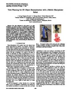
I. I NTRODUCTION As virtual reality, augmented reality and teleoperation applications demand even more realistic 3D models, we address in this paper the problem of reconstructing a complex shape object placed on a turntable from its sequence of images taken by a digital camera (see figure 1).
Fig. 1.
Turntable system overview (e.g. [1]).
Turntable systems have been used in numerous graphics and computer vision papers to compute the 3D reconstruction of 3D solid models by volume intersection from multiple views. Most authors use projective geometry properties and multiviews relations to perform the 3D reconstruction (e.g. [2] [3] [4]). These algorithms belong to a set of methods called Structure-From-Motion (SFM) techniques. The 3D reconstruction of an object, constrained to an axial rotation motion, is possible when the rotation axis does not go through the optical center of the camera. The existing algorithms can be included in two main categories : discreet approach and continuous approach. Under the expression discreet approach, we have the algorithms that treat the image sequence by taking the images n by n with n < 4 and with a large displacement between each view. Indeed, the images can be taken two by two to obtain the so-called Stereovision Approach (e.g. [5]), three by three for the Trifocal Approach (e.g.
[6]), and finally four by four for the Quadrifocal Approach (e.g. [7]). For the continuous approach, the image sequence is taken as a whole using time as an additional information. Known techniques are Optical Flow (e.g. [8]), Factorizationbased Reconstruction (e.g. [9]) and Filter-design Approach (e.g. [10]). For the single axis turntable approaches the authors in [11] present a two-stage technique. The first one is a grouping algorithm which operates on the spatiotemporal constraints associated with the axial motion to obtain a reliable description of the corresponding points through the image sequence as a conic trajectory. The reason of that choice is that the conic estimation algorithms are unstable when the trajectories of the image points are taken separately. The second stage gives the closed-form equations to estimate the motion and the 3D structure from the 2D (image) trajectories. In [3], the authors use a stereovision and trifocal approach to estimate the projection matrices associated to each image of the sequence. Then a Bundle Adjustment Algorithm (e.g. [12]) is used to minimize the re-projection error between the perspective projections of the estimated 3D points and their images. In [13], the conic estimation in directly made in 3D. A nonlinear criterion is used to obtain the 3D structure of the object. The camera is supposed to be fully calibrated. From the projective properties of the conics and their estimation in the image, the authors in [14] find the associated 3D circle. A non-linear criterion obtained from the projective invariants and the conics is minimized over 6 + 2n (n is the number of conics) parameters. The algorithm is initialized by using several points which have the longest trajectories through the sequence. When an object is placed on a turntable and is rotating around a single axis, all its points describes 3D circles. Their projections on the camera are conics entities in the general case. Therefore the idea in that paper is to understand the properties of the geometric locus through the sequence in order to start from a two dimensions space (the 2D conics) and to arrive to a tri dimensions result (the 3D circles). II. S INGLE A XIS GEOMETRY A. Camera Model The model of the camera used in this paper is the wellknown Pinhole Camera Model (e.g. [15]) which describes the
perspective projection model. From a mathematical point of view, the perspective projection is represented by the projection matrix P of size 3 × 4 ˜ = [X, Y, Z, 1]t , which makes corresponding to 3D points M t ˜ = [u, v, 1] . λ is a scale factor (an arthe 2D image points m bitrary positive scalar) used for the homogeneous coordinates representation : ˜ ˜ = PM λm
(1)
The projection matrix P encapsulates the extrinsic parameters (camera position and orientation) and the intrinsic parameter (the focal length fc ) by considering that the principal point has the coordinates [u0 , v0 ]t = 0t : fc R11 fc R12 fc R13 fc T x (2) P = fc R21 fc R22 fc R23 fc T y R31 R32 R33 Tz
We suppose that the camera is fully calibrated (intrinsic and extrinsic parameters known) and this can be done using the algorithm we have presented in [16] or using a classical calibration method (e.g. [17]).
δ = 4AC − B 2 = R2 (R33 2 − 1) + R33 h + Tz 2 > 0
Consequently, if that constraint is respected for the values of R and h, the image will be necessarily an ellipse. The constraint, expressed by equation (4), makes that the radius of the 3D circle is always contained between the rotation axis of the object and the image plane. Therefore, the image can not be different from an ellipse (point, line, parabola, hyperbola). Each component of the relations defined in equation (3) can be written as follow : A B C 2 2 (5) D = V1 · R + V2 · h + V3 · h + V4 E F The coefficients (A, B, C, D, E, F ) are the same (up to a scale factor) that the one estimated from the image points using a conic estimation algorithm (e.g. [18]). III. 3D R ECONSTRUCTION
B. Conics as Circle Perspective Projection A 3D circle can be defined as the intersection of a plane and a sphere (see figure 2). Using the perspective projection relation, the image of the 3D circle has the following equation (e.g. [16]) : C(u, v) = A · u2 + B · u · v + C · v 2 + D · u + E · v + F = 0 (3) The conic coefficients A to F are function of the focal length fc , one of the column of the rotation matrix (the normal n to the plane supporting the 3D circle, e.g. n = [R13 , R23 , R33 ]t ), the translation vector Tx , Ty , Tz , the radius R of the circle and the height h at which the circle is along the normal (Z axis) in a reference frame fixed by the calibration step (see figure 2). Camera
S
Rc
(4)
Π R ~n C h
A. Radius and Height calculous The previous section has shown that when an object is constraint to an axis rotation motion, its points describe circles. Their projections are then, staying in our hypothesis, ellipses, which have the following equation : C(u, v) = R2 + α1 (u, v)h2 + α2 (u, v)h + α3 (u, v) = 0 (6) where f (u, v, Vi+1 (j)) αi (u, v) = g(u, v, V1 (j))
(7)
with Vi (j) the jth component of the vector V i defined in relation (5). The functions f and g are quadratic functions in u and v obtained from equations (5) and (6). That ellipse is partially visible due to occultations (part of the ellipse is not visible). Therefore, to estimate the radius and the height of the 3D corresponding circle, an objective function has to be defined and will be minimized over the N points of the image trajectory in accordance with equation (6). That function can be written as follow :
Z Y X
Rs
J(R, h) =
N X
2
2
2
[R + α1 (ui , vi )h + α2 (ui , vi )h + α3 (ui , vi )] → 0 (8)
i=1
Fig. 2.
Geometric definition of a 3D circle in a reference frame.
The equation (3) is a conic equation. That conic is an ellipse when δ = 4AC − B 2 > 0. That constraint, after some simplifications, can also be expressed as a function of the radius and the height of the corresponding 3D circle, and the extrinsic and intrinsic camera parameters :
The minimum of that function is obtained by calculating its partial derivatives in R and h and finding their zeros. For clarity in the equations, the following notation will be used : N X i=1
αj (ui , vi ) ⇐⇒
X
αj
(9)
The system of equations linked to the partial derivatives is the following :
∂J(R, h) ∂R2 ∂J(R, h) ∂h
= =
N R 2 + h2 2h3
X
X
+
h(
+
X
X
α21
α22
α1 + h
+ 3h
+2
2
X
α2 α3 + R 2 (
X
X
α2 +
X
α3 = 0
min(h,R) {J(R, h) =
α1 α2
α2 + 2h
α1 ) = 0 (10)
ah3 + bh2 + ch + d = 0
(11)
with X
X 2N α12 − 2( α1 )2 X X X 3(N α1 α2 − α1 α2 ) X X 2 N( α2 + 2 α1 α3 ) X X X α3 − ( α2 )2 2 α1 X X X α3 N α2 α3 ) − α2
(12)
2
b When we have 4p3 + 27q 2 < 0 with p = ac − 3a 2 and 2 b b 9c d q = 27a (2 a2 − a ) + a , the equation (11) gives three real solutions. The solution to take is the one which minimize the equation (8). From the solution h obtained, the value of the radius R can be found using the first equation in the system (10). It is important to notice that a minimum of two points is needed (N ≥ 2) to get a solution. Another approach consist of using an iterative algorithm of minimization under constraint on equation (8). The best constraint is δ, defined in equation (4) which imposes the solution to be an ellipse. The criterion to be used in the objective function is based on the algebraic distance and to integrate the constraint δ, an interior penalization of Hyperbolic type method can be applied (e.g., [19]) :
min(R,h) {J(R, h) −
[(ui − uˆi )2 + (vi − vˆi )2 ]}
(14)
B. Angle Shift Estimation X
By isolating R2 in the first line of the system (10) and by injecting it in the second equation, the following expression of degree 3 in h is obtained :
a = b = c = − d =
N X i=1
α1 α3 )
X
(center, orientation and axes length) obtained for the conic coefficients (see equation (3)) :
λ } δ(R, h)
The camera is supposed to be calibrated : the intrinsic and extrinsic parameters are known. From the previous section, the radius and the height of the 3D circle supporting the 3D point to estimate are known. The coordinates of the 3D point can be calculated as follow using the polar coordinates : X = R cos(β ± i∆θ) Y = R sin(β ± i∆θ) (15) Z = h
where i is the image number in the sequence and ∆θ is the value of the rotation step of the turntable. Using the perspective projection defined by equation (1) and injecting in it equation (15), one obtains the estimated image coordinates of the 3D points : uˆ i vˆi
= fc
R11 X + R12 Y + R13 h + Tx R31 X + R32 Y + R33 h + Tz
(16)
R21 X + R22 Y + R23 h + Ty = fc R31 X + R32 Y + R33 h + Tz
The value of β to choose is the one which minimize the following criterion based on the euclidean distance between the re-projected estimated point and the original starting image point of the circular trajectory in the sequence : K(β) = min(β)
X
[(ui − uˆi )2 + (vi − vˆi )2 ]
(17)
It is important to notice that a value of β can be obtained directly from the equation (16). The problem is that the result is calculated from the inverse tangent function and therefore an ambiguity come out from the estimated angle. It is why it is simpler to use a minimization scheme on the criterion given in equation (17).
(13)
It is clear that with that formulation, the limit δ = 0 is not reachable because it corresponds to an infinite criterion, therefore if the algorithm is initialized with admissible values of R and h, it is impossible to go out from the admissible domain. Furthermore, when δ < 0 the criterion increases and penalizes the function. As an initial value, we set δ = 1 as suggested in [20] to guarantee the obtention of an ellipse. The objective function J(R, h) is minimized using the well-known Levenberg-Marquardt algorithm (e.g. [19]). The parameter λ is a tuning parameter to enforce the constraint δ. The objective function can also be based on the geometric distance which is calculated using the ellipse characteristics
C. 3D Reconstruction Algorithm The algorithm for the 3D reconstruction of solid objects placed on a turntable, is summarized as follows : • Recover calibration parameters using the algorithm presented in [16] or [17]. For each trajectory (e.g. [22] for tracking algorithm), • Choose initial height hinit = 0 and initial radius Rinit = s 1 − Tz2 | | to respect the constraint δ . R33 2 − 1 • Solve the system of equations (10) or minimize equation (13) with λ = 100 and δ(R, h) = equation (4) using the Levenberg-Marquardt algorithm (e.g. [19]).
This part shows the robustness of our algorithm to image noise and hidden parts of the circle to be reconstructed. The simulations have been carried out as follows : • Two circles of known radii are used for calibration (e.g. [16]). • A white gaussian noise from 0 to 5 pixels has been added to image data. • 100 trials have been realized to calculate the average relative error on the estimation of the radius R and the height h as shown in figure 4. Four configurations have been taken into account as shown in figure 3. Therefore different circle radii and heights have been considered with different visible portions.
0 −100 −200
Configuration 1
Relative Error (in %)
Relative Error (in %) 0
1
2
3
4
5
5 0
0
1
Relative Error (in %)
Configuration 2
Relative Error (in %)
8 6 4 2 0
0
1
2
3
4
5
Relative Error (in %)
Configuration 3
8 6 4 2 0
1
2
3
4
5
30 20 10 1
2
3
Noise (in pixels)
Fig. 4. level.
5
4
5
4
5
4
5
10 5 0
0
1
2
3
20 15 10 5 0
0
1
2
3
Noise (in pixels)
40
0
4
15
Noise (in pixels) 50
0
3
20
Noise (in pixels)
10
0
2
Noise (in pixels)
10
4
5
20 15 10 5 0
0
1
2
3
Noise (in pixels)
Relative error on radius and height reconstruction compare to noise
in C++ and placed in a configuration of a turntable system. The first image of the sequence is given in figure 5. The two circles on the support plane are used for the calibration.
100 0 −100 −200
Fig. 5.
−300
0
500
−500
0
u (in pixels)
u (in pixels)
Configuration 3 : R=30, h=50.
Configuration 4 : R=30, h=50.
300
200
200
100 0 −100 −200 −300
v (in pixels)
300
144°