Tutorial #1402: Training Simulation Fidelity – Establishing Preferences, Priorities, and Optimizing Trade-offs Kevin F. Hulme, New York State Center for Engineering Design and Industrial Innovation (NYSCEDII) Kemper E. Lewis, Department of Mechanical and Aerospace Engineering, University at Buffalo
Learning Objectives
Understand how the concept of “Fidelity” is relevant in the M&S community as it pertains to training Recognize how Fidelity often leads to a trade-off between training effectiveness, cost, and other factors Distinguish techniques to analyze (or optimize) training solution (Fidelity) alternatives Comprehend the efficacy of establishing priorities on three Fidelity case studies 2
Outline of Topics
Tutorial Overview and Introduction Motivation Fidelity – An Overview Establishing Preferences and Priorities in Simulation Case Studies 1: Civilian Simulation in Driver Training (Pareto Analysis) 2: Mitigating Simulator Sickness in Flight Training (Design of Experiments) 3: Training Simulator Features (Analytic Hierarchy Process)
Summary and Conclusions Acknowledgements Bibliography 3
I. Overview and Introduction
“Fidelity” – concept definition • A measure of the realism of a model or simulation • The degree of similarity between training and reality “The accuracy of the representation when compared to the real world”
REF: DoD Directive 5000.59-P, DoD M&S Master Plan, (1995)
REF: Hays, R.T., and Singer, M.J., (1988)
4
I. Overview and Introduction
Example: Fidelity in Computer Games (“Tennis”) 1975 1985 1995 2005 2015 5
I. Overview and Introduction
Relevance: how does “Fidelity” relate to M&S?
• •
1
Fidelity
The importance of various aspects of fidelity depend on the intended learning outcome(s) of the simulation
0.5 0
Investment
One can expect diminishing returns at some point This must be determined by the M&S expert(s)
REF: Duncan, J., (2007)
6
II. Motivation
The evolutionary need for EFFECTIVE training
Simulators
REF: Dale, E. (1969)
7
II. Motivation
• • • • •
Pros of Simulation: Ability to fire weapons (usually restricted on the ranges) Overcome range/space limitations (e.g., large battlefields) Enables large units to create/refine crew coordination/teamwork Enables scenario rehearsal prior to conducting the mission Reduces wear and tear on equipment (aircraft, vehicles, ships)
Engagement - Simulators are a “fun” way to learn Safety - Gain hands-on experience of dangerous situations Training Cost - less expensive than using the real system REF: Tegler, E., (2011)
8
II. Motivation
Cons of Simulation: • Negative training – Simulators need to accurately represent the flight/travel envelope in all situations (e.g., Stall models) • Simulation sickness – a multitude of factors can cause unwanted side effects (i.e., flight, driving, entertainment Sims) • Acquisition Cost - A professional flight simulator can cost from “thousands” to “millions” of dollars to: – – – –
purchase the equipment, instrument the simulator cabin/vehicle, install and calibrate the data acquisition systems, and verify/validate the models and develop the training software.
REF: Levin, A., (2010) ; Johnson, D.M., (2005)
9
II. Motivation
Cost Considerations “A $20 million simulator will look a lot better than a $200,000 system. But do you need it?” “You can get 70% of the capability for 1/100th of the cost. It’s the other 30% that costs so much.” “We can create a (low cost environment) that accomplishes ~ 80% of what I need at $100,000, vs. 95% at $10 million. That opens the market for broader use of simulation…”
REF: Erwin, S.I., (2000)
10
II. Motivation
So, do the benefits outweigh the gains? For many, the entire decision necessarily boils down to COST vs. VALUE added… …but how is this determination made?
11
III. Fidelity – an Overview
What types of factors influence Fidelity? Cost concerns •
Simulators can be VERY expensive
Motion vs. no motion •
Does motion enhance the simulator experience?
Field-of-View (F.O.V.) •
The more that can be seen (peripheral, rear), the better
Size/footprint/portability •
Should simulator be fixed or transportable?
12
III. Fidelity – an Overview
(Low) Desktop Simulator Estimated Cost: $1,000 Advantages: Lowest cost, Portable Ideal for group training Disadvantages: Very low fidelity, Non-immersive Narrow field-of-view 13
III. Fidelity – an Overview
(Medium) Wide F.O.V. Standalone Simulator w/ “seat shaker” Estimated Cost: $50,000 Advantages: Large curved screen, Decent sense of immersion Disadvantages: Very limited motion, Not so portable 14
III. Fidelity – an Overview
(High) Moving track, Motion-based, Surround-screen Simulator Estimated Cost: > $1,000,000 Advantages: Surround F.O.V., ultra-realistic driving forces, “as good as driving” Disadvantages: Cost prohibitive, Consumes a full building 15
III. Fidelity – an Overview
Defining Fidelity (multiple dimensions) Simply defining system fidelity as low/medium/high can be inadequate. A more useful description of fidelity includes both qualitative and quantitative measures on multiple dimensions REF: Duncan, J., (2007)
16
III. Fidelity – an Overview
Fidelity: Physical vs. Functional (vs. Perceived) Physical: “does simulation look and feel real?” More critical in the case of reproductive skills (no cognition) Functional: “does simulation operate/respond realistically?” More critical in the case of productive skills (cognition)
Perceived: the extent to which the training device *appears* to look/feel and operate/respond real by the trainee. For effective training – this matters most!! REF: Allen, J.A., Hays, R.T., and Buffardi, L.C., (1986)
17
III. Fidelity – an Overview
Customer Requirements Def: What are the simulator features, functions, and attributes that are required for a specific training purpose? Customer/program manager: identify the training objectives for the student(s)/trainee(s). There will likely be trade-offs (e.g., cost, technology, reliability, sustainability) to achieve training objectives Simulator designer: objective is to help to identify a simulator design that meets their customer’s needs REF: Kotonya, G., and Sommerville, I., (1998)
18
III. Fidelity – an Overview
Customer Requirements (cont.) Customer:
Determine requirements to train basics
Determine requirements to perform mission
“good” Attain available resources for: or
iterate
“better”
iterate
or
Sim Designer:
“best”
Finalize design considering all factors (cost, fidelity, etc.) 19
III. Fidelity – an Overview
Section Summary • The choice of a simulator arrangement and features involves many fidelity-based decisions • Many fidelity-based decisions depend on the context of the training application - what is critical, and what is not? • Iteration between simulator expert and Customer should help to identify the “optimal” balance of needs So how are these types of decisions made?
20
IV. Establishing Preferences
Trade-off decision Defined: a situation that involves losing one quality/aspect of something in return for gaining another It often implies a decision to be made with full understanding of both the upside and downside of a particular choice
REF: Garland Jr., T., (2014)
21
IV. Establishing Preferences
Numerical Optimization • Many times, we are faced with a problem where we want to find the “best solution” • Sometimes this solution is of the form: Minimize or Maximize F(x)
REF: Vanderplaats, G.N., (1984)
22
IV. Establishing Preferences
Numerical Optimization (cont.) • F represents your objective or what you want to increase or decrease (e.g., cost, risk, performance, weight) • x represents the variables under your control (e.g., simulator type) F
F
Maximum
Minimum
x
x 23
IV. Establishing Preferences
Design of Experiments (DOE) • Orthogonal Arrays (OAs) – One type of DOE – Serve as a means of compressing the total number of experiments when the goal is to measure the contribution of each of several factors to a prescribed outcome
• The (orthogonal) sequence of trials is efficient: – Fewer test cases can dramatically reduce overall test cycle time
• OAs are culled from published lists that have been validated • Use Analysis of Variance (ANOVA) to determine the relative impact of each factor REF: Roy, R. (2001)
24
IV. Establishing Preferences
Design of Experiments L8 (27) OA - 8 experiments per array, with seven 2-level factors 27
• = 128 combinations (full factorial) • Each experiment (row) has an associated observation value (“objective function”)
L8
F1
F2
F3
F4
F5
F6
F7
1
1
1
1
1
1
1
1
2
1
1
1
2
2
2
2
3
1
2
2
1
1
2
2
4
1
2
2
2
2
1
1
5
2
1
2
1
2
1
2
6
2
1
2
2
1
2
1
7
2
2
1
1
2
2
1
8
2
2
1
2
1
1
2 25
IV. Establishing Preferences A. B. C. D.
E. F. G. H.
Gender Roll/Pitch/Yaw Heave/Surge/Sway Driver (D), Passenger (P)
Audio Cues Day (D) or Night (N) Forward F.O.V. Observation Value (or Objective Function) (0-100)
L8
A.
B.
C.
D.
E.
F.
G.
H.
1 2 3 4 5 6 7 8
M M M M F F F F
on on off off on on off off
on on off off off off on on
D P D P D P D P
on off on off off on off on
D N N D D N N D
60 180 180 60 180 60 60 180
91 68 24 77 82 55 49 39 26
IV. Establishing Preferences
Multi-objective decision making • When we have a single objective, F, the best solution can be found using derivative information ( F = 0 & ଶ F) • But what about when we have multiple objectives, F1 and F2? F1
F2
x
• This is relevant when choosing a simulator (or feature) • How do you choose the “best” solution in this case? REF: Marler, T., and Arora, J., (2009)
27
IV. Establishing Preferences
Pareto frontier of optimal options • A better way to visualize such tradeoffs is the following: F1 (fidelity)
Pareto frontier “utopia” point
(achievable)
(unachievable)
F2 (cost) REF: Pardalos, P., Migdalas, A., and Pitsoulis, L., (Eds.), (2008)
28
IV. Establishing Preferences
Identifying Best Options • Step 1: Identify all the possible options that are equal or worse than at least one other solution on both objectives • Step 2: Identify the Pareto, non-dominated frontier of options F1 (fidelity)
Set of dominated options
F2 (cost) 29
IV. Establishing Preferences
Identifying Best Options: Option Classes F1 (fidelity)
Class 1: Options not to consider Class 2: Those that fulfill cost priorities Class 3: Those that fulfill fidelity priorities Class 4: Those that fulfill blended priorities F2 (cost) 30
IV. Establishing Preferences
Establishing Priorities (pairwise) • To establish/reveal your priorities, pose a few problems using hypothetical simulators/features Option B
F1 (fidelity)
Option A
Which option do you prefer, A or B?
F2 (cost) 31
IV. Establishing Preferences
Opportunity Costs (and Trade-offs) • The "cost" incurred by not enjoying the benefit that would be had by taking the second best choice available • “The loss of potential gain from other alternatives" e.g., the costs associated with replacing staff during training
REF: Heymann, H.G., and Bloom, R., (1990)
e.g., the estimate of added value per trained employee
32
IV. Establishing Preferences
Cost-Value Approaches: Analytic Hierarchy Process (AHP) To assist decision-making, AHP compares feature types in a stepwise fashion and measures their relative contribution (both to VALUE and COST) Step 1: Set up (VALUE) requirements in an n x n matrix: Feature 1
Feature 2
Feature 3
Feature 4
Feature 1 Feature 2 Feature 3 Feature 4
REF: Karlsson, J., and Ryan, K., (1997) ; Saaty, T.L., (1980)
33
IV. Establishing Preferences
Analytic Hierarchy Process (AHP) Step 2: Perform pairwise Relative Intensity 1 comparison of each set 3 of requirements: 5 This is also called the “comparison matrix”
Definition Of equal value Slightly more value Strong value
7
Very strong value
9
Extreme Value
Feature 1
Feature 2
Feature 3
Feature 4
Feature 1
1
4
6
1/2
Feature 2
1/4
1
1/3
9
Feature 3
1/6
3
1
1/5
Feature 4
2
1/9
5
1 34
IV. Establishing Preferences
Analytic Hierarchy Process (AHP) Step 3: Attain sum of all columns Step 3a: Normalize each column (by its sum) Step 3b: Now sum across rows to estimate eigenvalues Step 3c: Divide by ‘n’ (matrix order) to get Priority Vector (PV) Step 4: PV helps to assign each feature a relative value: Eigenvalue: Feature 1
0.363
Feature 2
0.465
Feature 3
0.055
Feature 4
0.115
Value added: Feature 1, 36.3% Feature 2, 46.5% Feature 3, 5.5% Feature 4, 11.5% 35
IV. Establishing Preferences
Analytic Hierarchy Process (AHP) Step 5: Estimate numerical reliability of results: • Consistency Index: CI = (λmax- n)/(n -1) • Consistency Ratio (CR) = CI/RI ; must be < 0.10, where “RI” is the Random Index, defined by the following lookup table: Matrix order: RI:
1 0.00
2 0.00
3 0.58
4 0.90
5
6 1.12
7 1.24
1.32
• Repeat entire process using COST as a basis • Construct Cost-Value diagram to make trade-off decisions 36
IV. Establishing Preferences
Section Summary • The goal should be to make an optimal decision, maximizing or minimizing your objective(s) • Design of Experiments is an efficient method to minimize the total number of experiments • When there are more than one objective, the decision becomes an optimal trade-off • Opportunity Costs quantify the “loss of potential gain” • Analytic Hierarchy Process is an intuitive Cost-Value approach for decision-making 37
V. Case Study 1: Simulator Features
Pareto Frontiers Example Problem Statement: A driver training school wants to invest in simulators to reduce car crashes among its students. How long (in MONTHS) to “pay off” investment? Average insurance claims (2012) for: • • • •
Property damage: $3,073 Bodily injury: $14,653 Collision: $2,950 Comprehensive: $1,585
Equally weighted average for all 4 categories: $5,565 REF: Rocky Mountain Insurance Information Association, (2014)
38
V. Case Study 1: Simulator Features
Background data: Class Size (ANNUAL):
Small 100
Small‐Med Medium 500 1,000
Med‐Lg 5,000
Large 10,000
Simulator Effectiveness:
1.00%
2.50%
5.00%
7.50%
10.00%
Investment (cost/student/classroom):
$1,000
$10,000
$50,000
$100,000
$500,000
Effectiveness is assumed as a measure of a serious accident prevented, and thus, a cost reduction (to society) of $5,565 (i.e., using the RMIIA data)
39
V. Case Study 1: Simulator Features
Scenario #1: Small Class Size (100), Medium Investment ($50,000); vary the Effectiveness
40
V. Case Study 1: Simulator Features
Scenario #2: Large Class Size (10,000), Small Effectiveness (1.0%); vary the Investment
41
V. Case Study 1: Simulator Features
Scenario #3: Medium-Large Investment ($100,000), MediumLarge Effectiveness (7.5%); vary the Class Size
42
V. Case Study 2: Mitigating Simulator Sickness
DOE Example Problem Statement: Specify candidate features of a flight simulator intended for military pilot training. Rectify system features that are most/least conducive to simulator sickness. Use the L16 array (L16 (45)) • • •
16 experiments 5 factors 4 level settings
REF: Hulme, K.F., Guzy, L.T., and Kennedy, R.S., (2011)
43
V. Case Study 2: Mitigating Simulator Sickness
DOE Example •
Driving Environment (2011 experiment) –
• •
Modeled after local roadways - include streetlights (green) and stop signs (red)
Durations of drives: 5, 10, 15, or 20 minutes Objective Measure: MSAQ (0-1), pre- and post-experiment Activity
Duration
Informed Consent
10 minutes
Pre- Surveys (MSAQ)
5 minutes
Simulator experiments (2)
30 minutes
Participant rest
5 minutes
Post- Surveys (MSAQ)
5 minutes
Participant observation
5 minutes
TOTAL: 60 minutes 44
V. Case Study 2: Mitigating Simulator Sickness
Investigate 5 Factors: A: Scene Brightness, B: DOF Rate Limiting, C: Duration, D: Motion DOF’s, E: F.P.S. L16 (a)
A
B
C
D
E
L16 (b)
A
B
C
D
E
1
15%
20%
5
0
15
9
65%
20%
15
6
24
2
15%
100%
10
2
24
10
65% 100%
20
4
15
3
15%
150%
15
4
45
11
65% 150%
5
2
60
4
15%
200%
20
6
60
12
65% 200%
10
0
45
5
40%
20%
10
4
60
13
90%
20%
20
2
45
6
40%
100%
5
6
45
14
90% 100%
15
0
60
7
40%
150%
20
0
24
15
90% 150%
10
6
15
8
40%
200%
15
2
15
16
90% 200%
5
4
24 45
V. Case Study 2: Mitigating Simulator Sickness
DOE Example Objective Function – use the Motion Sickness Assessment Questionnaire (MSAQ), which measures 16 categories of sickness, with a cumulative score on a normalized (0-1) scale
REF: Gianaros, P.J. et al., (2001)
46
V. Case Study 2: Mitigating Simulator Sickness
• •
DOE Example Here, used 8 participants to complete the L16 array Each participant performs 2 “experiments” in the array L16 (a)
A
B
C
D
E
1
15%
20%
5
0
15
2 3
15%
100%
10
2
24
15%
150%
15
4
45
4
15%
200%
20
6
60
5
40%
20%
10
4
60
6 7
40%
100%
5
6
45
40%
150%
20
0
24
MSAQ overall scores PreMidPost0.118 0.153 0.208 0.111 0.111 0.125 0.125 0.194 0.278 0.153 0.181 0.160 0.243 0.243 0.563 0.125 0.111 0.132 0.111 0.389 0.160
8
40%
200%
15
2
15
0.111
0.167
0.160 47
V. Case Study 2: Mitigating Simulator Sickness
DOE Example Perform ANOVA to determine which Factor(s) are most critical
48
V. Case Study 3: AHP – Establishing Priorities
AHP Example Problem statement: Specify features of a training simulator acquisition. Use a Cost-Value approach to assist in making critical trade-off decisions. 1. 2. 3. 4. 5. 6. 7. 8.
Field-of-view (H): Narrow, Wide, Curved? Motion: None, 3-DOF, 6-DOF? Cabin type: Chair, A-pillar, Full vehicle? Terrain fidelity: Low, Intermediate, High? Audio: None, 2.0, or 5.1 sound? Engine Braking: None, Mild, Severe? Field-of-View (V): Narrow, Square, Surround? Brake Pedal Haptics: Off, Partial, Full? 49
V. Case Study 3: AHP – Establishing Priorities
AHP Example Comparison Matrix (Value)
FOV-H Motion Cabin Terrain Audio EB FOV-V Haptics
FOV-H Motion Cabin Terrain Audio 1.000 0.375 2.000 4.000 5.000 2.667 1.000 5.000 8.000 4.000 0.500 0.200 1.000 3.000 2.000 0.250 0.125 0.333 1.000 0.500 0.200 0.250 0.500 2.000 1.000 0.250 0.333 1.333 2.000 3.003 0.250 0.500 2.000 3.003 7.003 0.167 0.200 0.333 0.500 0.333 5.28 2.98 12.50 23.50 22.84
EB FOV-V Haptics 4.000 4.000 6.000 3.000 2.000 5.000 0.750 0.500 3.000 0.500 0.333 2.000 0.333 0.143 3.000 1.000 0.750 4.500 1.333 1.000 3.000 0.222 0.333 1.000 11.14 9.06 27.50
50
V. Case Study 3: AHP – Establishing Priorities
AHP Example Normalize columns, then attain row sums (eigenvalues) (Value) FOV-H
Motion
Cabin
Terrain
Audio
EB
FOV-V Haptics
FOV-H
0.189
0.126
0.160
0.170
0.219
0.359
0.442
0.218
Motion
0.505
0.335
0.400
0.340
0.175
0.269
0.221
0.182
Cabin
0.095
0.067
0.080
0.128
0.088
0.067
0.055
0.109
Terrain
0.047
0.042
0.027
0.043
0.022
0.045
0.037
0.073
Audio
0.038
0.084
0.040
0.085
0.044
0.030
0.016
0.109
EB
0.047
0.112
0.107
0.085
0.131
0.090
0.083
0.164
FOV-V
0.047
0.168
0.160
0.128
0.307
0.120
0.110
0.109
Haptics
0.032
0.067
0.027
0.021
0.015
0.020
0.037
0.036
1.883 2.427 0.689 0.335 0.445 0.819 1.148 0.254
51
V. Case Study 3: AHP – Establishing Priorities
AHP Example Divide by “n” (8) to attain the Priority Vector (Value): FOV-H Motion Cabin Terrain Audio EB FOV-V Haptics
0.235 0.303 0.086 0.042 0.056 0.102 0.144 0.032
Assure numerical reliability: • Consistency Index: 0.094 • Consistency Ratio: 0.067 (less than 0.10; Good!)
= 23.5% = 30.3% = 8.6% = 4.2% = 5.6% = 10.2% = 14.4% = 3.2%
52
V. Case Study 3: AHP – Establishing Priorities
AHP Example Repeat Process……..Comparison Matrix (Cost) FOV-H Motion Cabin Terrain Audio EB FOV-V Haptics
FOV-H Motion Cabin Terrain Audio 1.000 0.250 0.500 5.000 6.000 4.000 1.000 2.000 9.000 8.000 2.000 0.500 1.000 7.000 5.000 0.200 0.111 0.143 1.000 0.750 0.167 0.125 0.200 1.333 1.000 0.333 0.143 0.200 3.003 1.502 1.000 0.333 0.250 7.003 5.000 1.333 0.250 0.400 1.429 1.333 10.03 2.71 4.69 34.77 28.58
EB FOV-V Haptics 3.000 1.000 0.750 7.000 3.000 4.000 5.000 4.000 2.500 0.333 0.143 0.700 0.666 0.200 0.750 1.000 0.500 0.300 2.000 1.000 4.000 3.333 0.250 1.000 22.33 10.09 14.00
53
V. Case Study 3: AHP – Establishing Priorities
AHP Example Normalize columns, then attain row sums (eigenvalues) (Cost) FOV-H
Motion
Cabin
Terrain
Audio
EB
FOV-V Haptics
FOV-H
0.100
0.092
0.107
0.144
0.210
0.134
0.099
0.054
0.939
Motion
0.399
0.369
0.426
0.259
0.280
0.313
0.297
0.286
2.629
Cabin
0.199
0.184
0.213
0.201
0.175
0.224
0.396
0.179
1.772
Terrain
0.020
0.041
0.030
0.029
0.026
0.015
0.014
0.050
0.225
Audio
0.017
0.046
0.043
0.038
0.035
0.030
0.020
0.054
0.282
EB
0.033
0.053
0.043
0.086
0.053
0.045
0.050
0.021
0.383
FOV-V
0.100
0.123
0.053
0.201
0.175
0.090
0.099
0.286
1.127
Haptics
0.133
0.092
0.085
0.041
0.047
0.149
0.025
0.071
0.643
54
V. Case Study 3: AHP – Establishing Priorities
AHP Example Divide by “n” (8) to attain the Priority Vector (Cost): FOV-H Motion Cabin Terrain Audio EB FOV-V Haptics
0.117 0.329 0.221 0.028 0.035 0.048 0.141 0.080
Assure numerical reliability: • Consistency Index: 0.089 • Consistency Ratio: 0.063 (less than 0.10; Good!)
= 11.7% = 32.9% = 22.1% = 2.8% = 3.5% = 4.8% = 14.1% = 8.0%
55
V. Case Study 3: AHP – Establishing Priorities
AHP Example Finally, plot the Value-Cost Priority Vectors (pairs): Key: FOV-H Motion Cabin Terrain Audio EB FOV-V Haptics
F M C T A E V H
56
V. Case Studies
Section Summary • Used Pareto decision-making to specify a simulator for teen driver training and education – Used insurance figures to estimate the “cost” of lives saved
• Used Design of Experiments (and ANOVA) to look at the relative importance of military flight simulator features – Used MSAQ to measure the impact of simulator sickness from various simulator aspects
• Used Analytic Hierarchy Process (AHP) to look at the Cost-Value tradeoffs for specifying features for a training simulator – Used Comparison Matrices help to inform decision-making
57
VI. Summary and Conclusions
• •
• •
Fidelity…an important concept in M&S-based training A measure of the realism of a model or simulation The importance of various aspects of fidelity depend on the intended learning outcome(s) of the simulation MANY factors influence simulation fidelity The point of diminishing returns must be determined by the M&S expert(s), Customer Requirements, etc.
Maximize Value, Minimize Cost
58
VI. Summary and Conclusions
•
•
•
Training Effectiveness vs. Cost: a trade-off decision Simulation has become an essential component for effective training However, COST (pre- and post- system acquisition) is always a major consideration Training Effectiveness vs. Cost is a tug-of-war, largely driven by the FIDELITY of the chosen training system Acquisition Cost
Effectiveness Fidelity
59
VI. Summary and Conclusions
•
Establishment of Preferences and Priorities Concepts introduced for trade-off decision-making: − − − − −
•
Many fidelity-based decisions depend on − −
•
Multi-objective optimization and Sensitivity Analysis Pareto Frontiers Design of Experiments Opportunity Costs Analytic Hierarchy Process (AHP) The specific training objective(s) The context of the training application
One must understand the many impacts of fidelity, and conduct & evaluate tradeoffs, to find the Fidelity “Sweet Spot” 60
VII. Acknowledgments
- The Tutorial Subcommittee at I/ITSEC 2014 - Support from National Science Foundation’s Industry & University Cooperative Research Center (I/UCRC) - Moog, Inc. for ongoing technical/financial support - Dr. Edward Kasprzak (Milliken Research Associates) for ongoing technical consultation - Dr. Kemper E. Lewis for assisting with this presentation
61
VIII. Bibliography (1/3) Allen, J.A., Hays, R.T., and Buffardi, L.C., (1986). “Maintenance training simulator fidelity and individual differences in transfer of training”, Human Factors, 28, 497-509. Dale, E., (1969). “Audio-Visual Methods in Teaching (3rd ed.)”, Holt, Rinehart, & Winston, New York. DoD 5000.59-P, (1995). “Modeling and Simulation (M&S) Master Plan”, October, 1995. Duncan, J., (2007). “Fidelity versus Cost and its effect on Modeling & Simulation”, Command and Control Research and Technology Symposium, Newport, RI. Erwin, S.I., (2000). “$65K Flight Simulator Draws Skepticism From Military Buyers”, National Defense, November, 2000. Garland Jr., T., (2014). “Trade-offs”, Current Biology, Vol. 24, No. 2, pp. R60-R61, DOI: 10.1016/j.cub.2013.11.036 Gianaros, P.J., Muth, E.R., Mordkoff, J.T., Levine, M.E., and Stern, R.M., (2001). “A Questionnaire for the Assessment of the Multiple Dimensions of Motion Sickness”, Aviat Space Environ Med. Feb 2001; 72(2): 115–119.
62
VIII. Bibliography (2/3) Hays, R.T., and Singer, M.J., (1988). “Simulation Fidelity in Training System Design: Bridging the Gap Between Reality and Training”, Springer Verlag, ISBN: 0387968466. Heymann, H.G., and Bloom, R., (1990). “Opportunity Cost in Finance and Accounting”, Praeger, ISBN: 0899304001. Hulme, K.F., Guzy, L.T., and Kennedy, R.S., (2011). “Holistic Design Approach to Analyze Simulator Sickness in Motion-based Environments”, The Interservice/Industry Training, Simulation and Education Conference (I/ITSEC), Orlando, FL, November, 2011. Johnson, D.M., (2005). “Introduction to and Review of Simulator Sickness Research”, U.S. Army Research Institute for the Behavioral and Social Sciences, Research Report 1832, April 2005. Karlsson, J., and Ryan, K., (1997). “A Cost–Value Approach for Prioritizing Requirements”, IEEE Software, Vol. 14, No. 5. Kotonya, G., and Sommerville, I., (1998). “Requirements Engineering: Processes and Techniques”, Chichester, UK: John Wiley and Sons.
63
VIII. Bibliography (3/3) Levin, A., (2010). “Current simulators can mislead pilots”, USA Today Technology article. Marler, T., and Arora, J., (2009). “Multi-objective Optimization: Concepts and Methods for Engineering”, VDM Verlag, Saarbrucken, Germany. Pardalos, P., Migdalas, A., and Pitsoulis, L., (Eds.), (2008). “Pareto Optimality, Game Theory, and Equilibria (1st Edition)”, Springer New York. Rocky Mountain Insurance Information Association (RMIIA), (2014). “Cost of Auto Crashes and Statistics”, http://www.rmiia.org/auto/traffic_safety/Cost_of_crashes.asp. Roy, R., (2001). “Design of Experiments Using The Taguchi Approach: 16 Steps to Product and Process Improvement”, John Wiley & Sons, New York, NY. Saaty, T.L., (1980). “The Analytic Hierarchy Process”, McGraw-Hill, New York. Tegler, E., (2011). “Air Force Flight Simulators May Help Cut Training Costs”, Defense Media Network, November, 2011 Vanderplaats, G.N., (1984). “Numerical Optimization Techniques for Engineering Design”, McGraw-Hill Ryerson, University of Michigan.
64
Contact Information
Presenter and Primary Author: Kevin F. Hulme, Ph.D. Senior Research Associate New York State Center for Engineering Design and Industrial Innovation (NYSCEDII) University at Buffalo Buffalo, NY 14260-1810 e-mail:
[email protected] Tel: 716-645-5573 65