This tutorial is designed to give you practice in fitting logistic models with
categorical ... This data set contains 7 variables: dust, race, sex, smoking, employ
,.
DEPARTMENT OF STATISTICS Course STATS 330: Advanced Statistical Modelling Tutorial Sheet 8: September 30, 2010 This tutorial is designed to give you practice in fitting logistic models with categorical explanatory variables (binary anova). In this tutorial you will investigate data from a survey of workers in the US cotton industry. The data records whether the workers were suffering from a lung disease called byssinosis. Also recorded were the values for five categorical explanatory variables: the race, sex and smoking status of the worker, the length of employment and the amount of dust in the workplace. The amount of dust in the workplace is thought to be a major factor in the occurrence of byssinosis but the other measured variables may also have an impact. The data has been put into a file called byssinosis.txt which can accessed from the webpage. This data set contains 7 variables: dust, race, sex, smoking, employ, yes and total. The first five of these are the categorical explanatory variables which have the following codings for their levels: dust race sex smoking employ
amount of dust in workplace: 1-high, 2-medium, 3-low. ethnic origin of worker: 1-white, 2-other. sex of worker: 1-male, 2-female. smoking status: 1-smoker, 2-nonsmoker. years of employment: 1-less than 10, 2-10 to 20, 3-more than 20.
For each combination of the explanatory variables, total represents the total number of workers and yes represent the number that suffer from byssinosis. This is grouped data. We will use binary ANOVA to investigate the relationship between the explanatory variables and the occurrence of byssinosis. Primary interest is in how the incidence of byssinosis is affected by the amount of dust in the workplace but the other variables need to be taken into account as well. You need to fit a model that explains the connection between the probability of contracting byssinosis and the other variables. You should run suitable diagnostic checks for your fitted model.
-1-
Task 1: Read in the data and create a suitable data frame for the analysis This should be routine by now. The data is found in “Data for past assignments”; it was assignment 4 in 2001. Caution: since the factors are coded as integers, you will need to make sure that the explanatory variables are converted to factors. See tutorial sheet 6, and below.
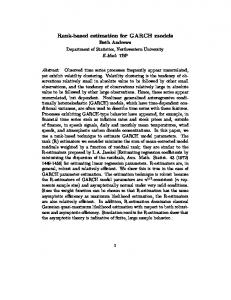
Task 2: Plot the data A good plot is that drawn by the plot.design function. (See lecture 24). You will need to use the logits (log-odds) of the different factor level combinations. It is helpful to create a new data frame, which includes the logits, and also recodes the categorical variables with more meaningful labels than 1, 2 or 3. This can be done with the data.frame function. Note the use of labels to recode the factors. The following assumes we have attached the original data frame. tut8.df20
other
-3.0
10-20 female
smoker
male nonsmoker medium white
-3.5
mean of est.logits
-2.0
high
|z|) (Intercept) -1.7529 0.1564 -11.207 < 2e-16 *** dustmedium -3.2770 0.5101 -6.424 1.33e-10 *** dustlow -2.8783 0.2422 -11.883 < 2e-16 *** smokingnonsmoker -0.6578 0.1945 -3.382 0.000719 *** employ10-20 0.4640 0.2512 1.847 0.064704 . employ>20 0.6367 0.1836 3.467 0.000526 *** sexfemale -0.9990 0.6106 -1.636 0.101792 dustmedium:sexfemale 2.0056 0.8309 2.414 0.015791 * dustlow:sexfemale 1.2576 0.6823 1.843 0.065286 . --Signif. codes: 0 `***' 0.001 `**' 0.01 `*' 0.05 `.' 0.1 ` ' 1 (Dispersion parameter for binomial family taken to be 1) Null deviance: 322.527 Residual deviance: 36.019 AIC: 160.69
on 64 on 56
degrees of freedom degrees of freedom
-3-
Task 4. Interpret the coefficients Take careful note of which factor levels are the baseline. For example, the baseline for dust is “high”. The coefficients for dustmedium and dustlow are negative, so high dust is clearly more harmful than low or medium dust. Also, the probability increases as the length of exposure increases. How would you interpret the dust:sex interaction?
Task 5: check the model Run the diagnostics. Is the deviance OK? Any strange points? Refer to Arden’s model answers to assignment 4, 2001 for more details.
-4-