Tutorial in Joint Modeling and Prediction: a statistical software ... - arXiv

arXiv:1701.03675v1 [stat.CO] 13 Jan 2017

Tutorial in Joint Modeling and Prediction: a Statistical Software for Correlated Longitudinal Outcomes, Recurrent Events and a Terminal Event Agnieszka Kr´ ol

Audrey Mauguen

Yassin Mazroui

ISPED, INSERM U897 Université de Bordeaux


Université Pierre et Marie Curie & INSERM, UMR S 1136, Paris

Alexandre Laurent

Stefan Michiels

Virginie Rondeau


INSERM U1018, CESP & Gustave Roussy, Villejuif


Abstract Extensions in the field of joint modeling of correlated data and dynamic predictions improve the development of prognosis research. The R package frailtypack provides estimations of various joint models for longitudinal data and survival events. In particular, it fits models for recurrent events and a terminal event (frailtyPenal), models for two survival outcomes for clustered data (frailtyPenal), models for two types of recurrent events and a terminal event (multivPenal), models for a longitudinal biomarker and a terminal event (longiPenal) and models for a longitudinal biomarker, recurrent events and a terminal event (trivPenal). The estimators are obtained using a standard and penalized maximum likelihood approach, each model function allows to evaluate goodness-of-fit analyses and plots of baseline hazard functions. Finally, the package provides individual dynamic predictions of the terminal event and evaluation of predictive accuracy. This paper presents theoretical models with estimation techniques, applies the methods for predictions and illustrates frailtypack functions details with examples.

Keywords: dynamic prediction, frailty, joint model, longitudinal data, predictive accuracy, R, survival analysis.

1. Introduction Joint models Recent technologies allow registration of greater and greater amount of data. In the medical research different kinds of patient information are gathered over time together with clinical outcome data such as overall survival (OS). Joint models enable the analysis of correlated data of different types such as individual repeated data, clustered data together with OS. The repeated data may be recurrent events (e.g., relapses of a tumor, hospitalizations, appearance of new lesions) or a longitudinal outcome called biomarker (e.g., tumor size, prostate-specific

2

Joint Modeling and Prediction

antigen or CD4 cell counts). The correlated data that are not analyzed jointly with OS, are subjugated to a bias coming from ignoring the terminal event which is the competing event for the occurrence of repeated outcomes (not only it precludes the outcomes from being observed but also prevents them from occurring). On the other hand, the standard survival analysis for OS may lead to biased estimations, if the repeated data is considered as time-varying covariates or if it is completely ignored in the analysis. For these correlated data one can consider joint models, e.g., a joint model for a longitudinal biomarker and a terminal event, which received the most of the attention in the literature. This joint model estimates simultaneously the longitudinal and survival processes using the relationship via a latent structure of random-effects (Wulfsohn and Tsiatis 1997). Extensions of these include, among others, models for multiple longitudinal outcomes (Hatfield, Boye, Hackshaw, and Carlin 2012), multiple failure times (Elashoff, Li, and Li 2008) and both (Chi and Ibrahim 2006). A review of the joint modeling of longitudinal and survival data was already given elsewhere (McCrink, Marshall, and Cairns 2013; Lawrence Gould, Boye, Crowther, Ibrahim, Quartey, Micallef, and Bois 2014; Asar, Ritchie, Kalra, and Diggle 2015). Another option for the analysis of correlated data are joint models for recurrent events and a terminal event (Liu, Wolfe, and Huang 2004; Rondeau, Mathoulin-Pélissier, Jacqmin-Gadda, Brouste, and Soubeyran 2007). These models are usually called joint frailty models as the processes are linked via a random effect that represents the frailty of a subject (patient) to experience an event. They account for the dependence between two survival processes quantified by the frailty term, contrary to the alternative marginal approach (Li and Lagakos 1997), which do not model the dependence. Some extensions to joint frailty models include incorporation of a nonparametric covariate function (Yu and Liu 2011), inclusion of two frailty terms for the identification of the origin of the dependence between the processes (Mazroui, Mathoulin-Pélissier, Soubeyran, and Rondeau 2012), consideration of the diseasespecific mortality process (Belot, Rondeau, Remontet, Roch, and CENSUR working survival group 2014) and accommodation of time-varying coefficients (Yu, Liu, Bravata, and Williams 2014; Mazroui, Mauguen, Macgrogan, Mathoulin-Pélissier, Brouste, and Rondeau 2015). Finally, Mazroui, Mathoulin-Pélissier, Macgrogan, Brouste, and Rondeau (2013) proposed a model with two types of recurrent events following the approach of Zhao, Liu, Liu, and Xu (2012). A review of joint frailty models in the Bayesian context was given by Sinha, Maiti, Ibrahim, and Ouyang (2008). Joint models for recurrent events and longitudinal data have received the least attention among the joint models so far. However, a marginal model based on the generalized linear mixed model was proposed by Efendi, Molenberghs, Njagi, and Dendale (2013). This model allows several longitudinal and time-to-event outcomes and includes two sets of random effects, one for the correlation within a process and between the processes, and the second to accommodate for overdispersion. Finally, in some applications all the types of data, i.e., a longitudinal biomarker, recurrent events and a terminal event can be studied so that all of them are correlated to each other (in the following we call such models trivariate models). Liu, Huang, and O’Quigley (2008) proposed a trivariate model for medical cost data. The longitudinal outcomes (amount of medical costs) were reported at informative times of recurrent events (hospitalizations) and were related to a terminal event (death). The dependence via random effects was introduced so that the process of longitudinal measurements and the process of recurrent events were related to the process of the terminal event. A relationship between longitudinal outcomes and

Agnieszka Król, Audrey Mauguen, Yassin Mazroui, Alexandre Laurent, Stefan Michiels, Virginie Rondeau 3 recurrent events was not considered. This relationship was incorporated to a trivariate model proposed by Liu and Huang (2009) for an application of an HIV study. In this parametric approach the focus was on the analysis of the associations present in the model and the effect of the repeated measures and recurrent events on the terminal event. Kim, Zeng, Chambless, and Li (2012) analyzed the trivariate data using the transformation functions for the cumulative intensities for recurrent and terminal events. Finally, Król, Ferrer, Pignon, Proust-Lima, Ducreux, Bouché, Michiels, and Rondeau (2016) proposed a trivariate model in which all the processes were related to each other via a latent structure of random effects and applied the model to the context of a cancer evolution and OS.

Prediction in joint models In the framework of joint models that consider a terminal event, one can be interested in predictions of the event derived from the model. As joint models include information from repeated outcomes, these predictions are dynamic, they change with the update of the observations. Dynamic predictive tools were proposed for joint models for longitudinal data and a terminal event (Proust-Lima and Taylor 2009; Rizopoulos 2011), joint models for recurrent events and a terminal event (Mauguen, Rachet, Mathoulin-Pélissier, MacGrogan, Laurent, and Rondeau 2013) and trivariate models (Król et al. 2016). For the evaluation of the predictive accuracy of a joint model few methods were proposed due to the complexity of the models in which the survival data are usually right-censored. The standard methods for the assessment of the predictive abilities derived from the survival analysis and adapted to the joint models context are the Brier Score (Proust-Lima and Taylor 2009; Mauguen et al. 2013; Król et al. 2016) and receiver operating characteristic (ROC) methodology (Rizopoulos 2011; Blanche, Proust-Lima, Loubère, Berr, Dartigues, and Jacqmin-Gadda 2015). Finally, the expected prognostic cross-entropy (EPOCE), a measure based on the information theory, provides a useful tool for the evaluation of predictive abilities of a model (Commenges, Liquet, and Proust-Lima 2012; Proust-Lima, Séne, Taylor, and Jacqmin-Gadda 2014).

Software for joint models Together with the theoretical development of the joint models, the increase of appropriate software is observed, mostly for standard frameworks. Among the R (R Development Core Team 2016) packages, the joint analysis of a single longitudinal outcome and a terminal event can be performed using JM (Rizopoulos 2016a) based on the likelihood maximization approach using expectation-maximization (EM) algorithm, JMbayes (Rizopoulos 2016b) built in the Bayesian context, and joineR (Philipson, Sousa, Diggle, Williamson, KolamunnageDona, and Henderson 2012), a frequentist approach that allows a flexible formulation of the dependence structure. For the approach based on the joint latent class models, i.e., joint models that consider homogeneous latent subgroups of individuals sharing the same biomarker trajectory and risk of the terminal event, an extensive package lccm (Proust-Lima, Philipps, Diakite, and Liquet 2016) provides the estimations based on the frequentist approach. Apart from the R packages, a stjm package (Crowther 2013) in STATA uses maximum likelihood and provides flexible methods for modeling the longitudinal outcome based on polynomials or splines. Another possibility for the analysis of the joint models for a longitudinal outcome and a terminal event is a SAS macro JMFit (Zhang, Chen, and Ibrahim 2014). Joint models

4


using nonlinear mixed-effects models can be estimated using MONOLIX software (Mbogning, Bleakley, and Lavielle 2015). Among the packages JM, JMbayes and lcmm provide predictive tools and predictive accuracy measures: EPOCE estimator in lcmm, ROC and AUC (area under the curve) measures and prediction error in JM and JMbayes. For joint models for correlated events (recurrent event or clustered event data) and a terminal event the available statistical software is limited. Among the R packages, joint.Cox (Emura 2016) provides the estimations using penalized likelihood under the copula-based joint Cox models for time to clustered events (progression) and a terminal event. Trivariate joint models proposed by Liu and Huang (2009) were performed in SAS using the procedure NLMIXED. The R package frailtypack (Rondeau, Gonzalez, Mazroui, Mauguen, Krol, Diakite, and Laurent 2016) fits several types of joint models. Originally developed for the shared frailty models for correlated outcomes it has been extended into the direction of joint models. These extensions include the joint model for one or two types of recurrent events and a terminal event, the joint model for a longitudinal biomarker and a terminal event and the trivariate model for a longitudinal biomarker, recurrent events and a terminal event. Moreover, frailtypack includes prediction tools, such as concordance measures adapted to shared frailty models and predicted probability of events for the joint models. Characteristics of a previous version of the package, such as estimation of several shared and standard joint frailty models using penalized likelihood, were already described elsewhere (Rondeau, Mazroui, and Gonzalez 2012). This work focuses on an overview and developments of joint models included in the package (model for recurrent/clustered events and a terminal event, model for multivariate recurrent events and a terminal event, model for longitudinal data and a terminal event and model for longitudinal data, recurrent events and a terminal event) and the prediction tools accompanied by predictive accuracy measures. Finally, several options available for the models (e.g., two correlated frailties in the model for recurrent events and a terminal event, left-censoring for the longitudinal data) will be presented with the appropriate examples. A practical guide to different types of models included in the package along with available options is presented in a schematic table in Appendix A. This article firstly presents joint models with details on estimation methods (Section 2) and predictions of an event in the framework of these joint models (Section 3). In Section 4, the frailtypack package features are detailed. Section 5 contains some examples on real datasets and finally, Section 6 concludes the paper.

2. Models for correlated outcomes 2.1. Bivariate joint frailty models for two types of survival outcomes a) Joint model for recurrent events and terminal event We denote by i = 1, . . . , N the subject and by j = 1, . . . , ni the rank of the recurrent event. For each subject i we observe the time of the terminal event Ti = min(Ti∗ , Ci ) with Ti∗ the true terminal event time and Ci the censoring time. We denote the observed recurrent times Tij = min(Tij∗ , Ci , Ti∗ ) with Tij∗ the real time of recurrent event. Thus, for each rank j we can summarize the information with a triple {Tij , δij , δi }, where δij = I{Tij =Tij∗ } and δi = I{Ti =Ti∗ } .

Agnieszka Król, Audrey Mauguen, Yassin Mazroui, Alexandre Laurent, Stefan Michiels, Virginie Rondeau 5 Let r0 (.) and λ0 (.) be baseline hazard functions related to the recurrent and terminal events, respectively. Let XRij and XT i be two vectors of covariates associated with the risk of the related events. Let β R and β T be constant effects of the covariates whereas β R (t) and β T (t) denote a time-dependent effect. Finally, a frailty ui is a random effect that links the two risk functions and follows a given distribution D and α is a parameter allowing more flexibility. The hazard functions are defined by (Liu et al. 2004; Rondeau et al. 2007): rij (t|ui ) = ui r0 (t) exp(X > Rij β R ) = ui rij (t) (recurrent event) , (1) α α λi (t|ui ) = ui λ0 (t) exp(X > (terminal event) T i β T ) = ui λi (t) where the frailty terms ui are iid (independent and identically distributed) and follow either the Gamma distribution with unit mean and variance θ (θ > 0), i.e., ui ∼ G( 1θ , 1θ ), or the lognormal distribution, i.e., ui = exp(vi ) ∼ lnN (0, σv2 ). The parameter α determines direction of the association (if found significant) between the processes. (1)

(1)

For a given subject we can summarize all the information with Θi = {T i , Ti , δ i , δi }, where (1) (1) T i = {Tij , j = 1, . . . , ni } and δ i = {δij , j = 1, . . . , ni }. Finally, we are interested to estimate ξ = {r0 (·), λ0 (·), β R , β T , θ, α}. In some cases, e.g., long follow-up, effects of certain prognostic factors can be varying in time. For this reason a joint model with time-dependent coefficients was proposed by Mazroui et al. (2015). The coefficients β R (t) and β T (t) are modeled with regression B-splines of order q and d is m interior knots. The general form of an estimated time-dependent coefficient β(t) d = β(t)

m X

ζbj Bj,q (t),

j=−q+1

where Bj,q (t) is the basis of B-splines calculated using a recurring expression (De Boor 2001). Therefore, for every time-varying coefficient, m + q parameters ζj , j = −q + 1, . . . , m need to be estimated. It has been shown that quadratic B-splines, i.e., q = 3, with a small number of interior knots (m ≤ 5) ensure stable estimation (Mazroui et al. 2015). The pointwise confidence intervals for β(t) can be obtained using the Hessian matrix. The application of time-varying coefficients is helpful if there is a need to verify the proportional hazard (PH) assumption. Using a likelihood ratio (LR) test, the time-dependency of a covariate can be examined. A model with the time-dependent effect and a model with the constant effect are compared and the test hypotheses depend on whether the covariate is related to one of the events or both. If the time-dependency is tested for both events the null hypothesis is H0 : βR (t) = βR , βT (t) = βT and the alternative hypothesis is H1 : βR (t) 6= βR , βT (t) 6= βT . The LR statistic has a χ2 distribution of degree k(m + q − 1), where k is the number of events to which the covariate is related. The LR test can also be used to verify whether a covariate with the time-dependent effect is significant for the events. In this case, a model with the time-varying effect covariate is compared to a model without this covariate. Again, the null hypotheses depend on the events considered. If the covariate is associated to both events, the null hypothesis H0 : βR (t) = 0, βT (t) = 0 is against H1 : βR (t) 6= 0, βT (t) 6= 0. The LR statistic has a χ2 distribution of degree k(m + q).

b) Joint model for two clustered survival events An increasing number of studies favor the presence of clustered data, especially multi-center

6


or multi-trial studies. In particular, meta-analyses are used to calculate surrogate endpoints in oncology. However, the clustering creates some heterogeneity between subjects, which needs to be accounted for. Using the above notations, the clustered joint model is similar to the model (1) but here, the index j (j = 1, . . . , ni ) represents a subject from cluster i (i = 1, . . . , N ) and the cluster-specific frailty term ui is shared by the subjects of a given group. Thus, the model can be written as (Rondeau, Pignon, and Michiels 2011): rij (t|ui ) = ui r0 (t) exp(X > (Time to event 1) Rij β R ) = ui rij (t) , > α α λij (t|ui ) = ui λ0 (t) exp(X T ij β T ) = ui λij (t) (Time to event 2) and we assume iid the Gamma distribution for the frailty terms ui . The events can be chosen arbitrarily but it is assumed that the event 2 impedes the process of the event 1. Usually the event 2 is death of a patient and the other is an event of interest (e.g., surrogate endpoint for OS) such as time to tumor progression or progression-free survival. The interest of using the joint model for the clustered data is that it considers the dependency between the survival processes and respects that event 2 is a competitive event for event 1. The frailty term ui is common for a given group and represents the clustered association between the processes (at the cluster level) as well as the intra-cluster correlation. The package frailtypack includes clustered joint models for two survival outcomes in presence of semi-competing risks (time-to-event, recurrent events are not allowed). To ensure identifiability of the models, it is assumed that α = 1. For these models, only Gamma distribution of the frailty term is implemented in the package.

c) Joint model for recurrent events and a terminal event with two frailty terms In Model (1) the frailty term ui reflects the inter- and intra-subject correlation for the recurrent event as well as the association between the recurrent and the terminal events. In order to distinguish the origin of dependence, two independent frailty terms ui = (ui ,vi ) can be considered (Mazroui et al. 2012): rij (t|ui ) = ui vi r0 (t) exp(X > Rij β R ) = ui vi rij (t) (recurrent event) , (2) > λi (t|ui ) = ui λ0 (t) exp(X T i β T ) = ui λi (t) (terminal event) where vi ∼ Γ( η1 , η1 ) (η > 0) specific to the recurrent event rate and ui ∼ Γ( 1θ , 1θ ) (θ > 0) specific to the association between the processes. The variance of the frailty terms represent the heterogeneity in the data, associated with unobserved covariates. Moreover, high value of the variance η indicates strong dependence between the recurrent events and high value of the variance θ indicates that the recurrent and the terminal events are strongly dependent. The individual information is equivalent to Θi from Model (1) and the parameters to estimate are ξ = {r0 (·), λ0 (·), β R , β T , θ, η}. In the package frailtypack for Model (2), called also general joint frailty model, only Gamma distribution is allowed for the random effects.

2.2. Multivariate joint frailty model One of extensions to the joint model for recurrent events and a terminal event (1) is consideration of different types of recurrence processes and a time-to-event data. Two types of recurrent events are taken into account in a multivariate frailty model proposed by Mazroui

Agnieszka Król, Audrey Mauguen, Yassin Mazroui, Alexandre Laurent, Stefan Michiels, Virginie Rondeau 7 et al. (2013). The aim of the model is to analyze dependencies between all types of events. (1) (1) (2) (2) The recurrent event times are defined by Tij (j = 1, . . . , ni ) and Tij (j = 1, . . . , ni ) and both processes are censored by the terminal event Ti . The joint model is expressed using the recurrent events and terminal event hazard functions:  (1) (1) (1) > (1) (1)   rij (t|ui , vi ) = r0 (t) exp(ui + X Rij β R ) = exp (ui )rij (t) (rec. event 1)  (2) (2) (2) > (2) (2) rij (t|ui , vi ) = r0 (t) exp(vi + X Rij β R ) = exp(vi )rij (t) (rec. event 2) ,    λi (t|ui , vi ) = λ0 (t) exp(α1 ui + α2 vi + X > T i β T ) = exp(α1 ui + α2 vi )λi (t) (terminal event) (3) (1) (2) (1) (2) with vectors of regression coefficients β R , β R , β T and covariates X Rij , X Rij , X T i for the first recurrent event, the second recurrent event and the terminal event, respectively. The frailty terms ui = (ui , vi )> explain the intra-correlation of the processes and the dependencies between them. For these correlated random effects the multivariate normal distribution of dimension 2 is considered: 2 ui σu ρσu σv , ui = ∼ N 0, vi ρσu σv σv2 Variances σu2 and σv2 explain the within-subject correlation between occurrences of the recurrent event of type 1 and type 2, respectively. The dependency between the two recurrent events is explained by the correlation coefficient ρ and the dependency between the recurrent event 1 (event 2) and the terminal event is assessed by the term α1 (α2 ) in case of significant variance σu2 (σv2 ). (1)

(2)

(1)

(2)

(l)

(l)

Here, for each subject i we observe Θi = {T i , T i , Ti , δ i , δ i , δi }, where T i = {Tij , j = (l)

(l)

1, . . . , ni } and δ i (1)

(2)

(l)

(l)

= {δij , j = 1, . . . , ni }, l = 1, 2 and the parameters to estimate are (1)

(2)

ξ = {r0 (·), r0 (·), λ0 (·), β R , β R , β T , σu2 , σv2 , ρ, α1 , α2 }.

2.3. Bivariate joint model with longitudinal data Here, instead of recurrent events we consider a longitudinal biomarker. For subject i we observe an li -vector of longitudinal measurements y i = {yi (tik ), k = 1, . . . , li }. Again, the true terminal event time Ti∗ impedes the longitudinal process and the censoring time does not stop it but values of the biomarker are no longer observed. For each subject i we observe Θi = {y i , Ti , δi }. A random variable Yi (t) representing the biomarker is expressed using a linear mixed-effects model and the terminal event time Ti∗ using a proportional hazards model. The sub-models are linked by the random effects ui = b> i :

Yi (t) = mi (t) + i (t) = X Li (t)> β L + Z i (t)> bi + i (t) (biomarker) , λi (t|bi ) = λ0 (t) exp(X T i > β T + h(bi , β L , Z i (t), X Li (t))> η T ) (death)

(4)

where X Li (t) and X T i are vectors of fixed effects covariates. Coefficients β L and β T are constant in time. Measurements errors i (·) are iid normally distributed with mean 0 and variance σ2 . We consider a q-vector of the random effects parameters bi = (b0 , . . . , bq−1 )> ∼ N (0, B1 ) associated to covariates Z i (t) and independent from the measurement error. In the frailtypack package, the maximum size of the matrix B 1 is 2. The relationship between the two processes is explained via a function h(bi , β L , Z i (t), X Li (t)) and quantified by coefficients

8


η T . This possibly multivariate function represents the prognostic structure of the biomarker mi (t) (we assume that the measurement errors are not prognostic for the survival process) and in the frailtypack these are either the random effects bi or the current biomarker level mi (t). The structure of dependence is chosen a priori and should be designated with caution as it influences the model in terms of fit and predictive accuracy. We consider that the longitudinal outcome yi (tik ) can be a subject to a quantification limit, i.e., some observations, below a level of detection s cannot be quantified (left-censoring). We introduce it in the vector y i which includes lio observed values y oi and lic censored values y ci (li = lio + lic ). The aspect of the left-censored data is handled in the individual contribution from the longitudinal outcome to the likelihood. The individual observed outcomes are Θi = {y oi , y ci , Ti , δi } (in case of no left-censoring y ci is empty and y oi is equivalent to y i ) and the parameters to estimate are ξ = {λ0 (·), β L , β T , B 1 , σ2 , η T }.

2.4. Trivariate joint model with longitudinal data The trivariate joint model combines the joint model for recurrent events and a terminal event (Model (1)) with the joint model for a longitudinal data and a terminal event (4). We consider the longitudinal outcome Y observed in discrete time points y i = {yi (tik ), k = 1, . . . , li }, times of the recurrent event Tij (j = 1, . . . , ni ) and the terminal event time Ti that is an informative censoring for the longitudinal data and recurrences. The respective processes are linked to each other via a latent structure. We define multivariate functions g(·) and h(·) for the associations between the biomarker and the recurrent events and between the biomarker and the terminal event, respectively. For the link between the recurrent events and the terminal event we use a frailty term vi from the normal distribution. This distribution was chosen here to facilitate the estimation procedure involving multiple numerical integration. Interpretation of vi should be performed with caution as the dependence between the recurrences and the terminal data is partially explained by the random-effects of the biomarker trajectory. We define the model by (Kr´ ol et al. 2016):  > (biomarker)  Yi (t) = mi (t) + i (t) = X Li (t) β L + Z i (t)> bi + i (t) > > r (t|vi , bi ) = r0 (t) exp(vi + X Rij β R + g(bi , β L , Z i (t), X Li (t)) η R ) (recurrent event) ,  ij λi (t|vi , bi ) = λ0 (t) exp(αvi + X T i > β T + h(bi , β L , Z i (t), X Li (t))> η T ) (terminal event) (5) where the regression coefficients β L , β R , β T are associated to possibly time-varying covariates X Li (t), X Rij , X T i for the biomarker, recurrent events and the terminal event (baseline prognostic factors), respectively. The strength of the dependencies between the processes is > quantified by α and vectors η R and η T . The vector of the random effects ui = (b> i , vi ) of dimension q = q1 + 1 follows the multivariate normal distribution: bi B1 0 ui = ∼ N 0, , vi 0 σv2 where the dimension of the matrix B1 in the frailtypack package is allowed to be maximum 2. It is convenient if one assume for the biomarker a random intercept and slope: Yi (t) = mi (t) + i (t) = X Li (t)> β L + bi0 + bi1 × t + i (t) and then bi0 represents the heterogeneity of the baseline measures of the biomarker among the subjects and bi1 the heterogeneity of the slope of the biomarker’s linear

Agnieszka Król, Audrey Mauguen, Yassin Mazroui, Alexandre Laurent, Stefan Michiels, Virginie Rondeau 9 trajectory among the subjects. As for Model (4) we allow the biomarker to be leftcensored, again with y oi the observed outcomes and y ci the undetected ones. For indi(1) (1) vidual i we observe then Θi = {y oi , y ci , T i , Ti , δ i , δi } and the interest is to estimate ξ = {r0 (·), λ0 (·), β L , β R , β T , B 1 , σv2 , σ2 , α, η R , η T }.

2.5. Estimation Maximum likelihood estimation Estimation of a model’s parameters ξ is based on the maximization of the marginal loglikelihood derived from the joint distribution of the observed outcomes that are assumed to be independent from each other given the random effects. Let ui represent random effects of a joint model (ui can be a vector, for Models (2), (3), (4), (5) or a scalar, for Model (1)) and fui (ui ; ξ) the density function of the distribution of ui . The marginal individual likelihood is integrated over the random effects and is given by: Z γ (2) γ (1) (2) (2) (1) (1) fyi |ui (y i |ui ; ξ)γL fT (1) |u (T i , δi |ui ; ξ) R fT (2) |u (T i , δi |ui ; ξ) R Li (Θi ; ξ) = i

ui

i

i

i

× fTi |ui (Ti , δi |ui ; ξ)fui (ui ; ξ) dui ,

(6)

where indicators γ· are introduced so that the likelihood is valid for all the joint models (1-5). Therefore, γL = 1 in case of Models (4) and (5) and 0 otherwise, γR(1) = 1 in case of the models (1), (3) and (5) and 0 otherwise, γR(2) = 1 in case of the model (3) and 0 otherwise. The conditional density of the longitudinal outcome fyi |ui is the density of the li -dimensional normal distribution with mean mi = {mi (tik ), k = 1, . . . , li } and variance σ2 I mi . In case of the left-censored data, we observe lio outcomes y oi and lic outcomes y ci are left-censored (below the threshold s). Then fyi |ui can be written as a product of the density for the observed outcomes (normal with mean mi (tik ) and variance σ2 ) and the corresponding cumulative distribution function (cdf) Fyi |ui for the censored outcomes: o

fyi |ui (y i |ui ; ξ) =

li Y k=1

c

fyio (tik )|ui (yio (tik )|ui ; ξ)

li Y

Fyic (tik )|ui (s|ui ).

k=1

Modeling of the risk of an event can be performed either in a calendar timescale or in a gap timescale. This choice depends on the interest of application whether the focus is on time from a fixed date, eg. beginning of a study, date of birth (calendar timescale) or on time between two consecutive events (gap timescale). The calendar timescale is often preferred in analyses of disease evolution, for instance, in a randomized clinical trial. In this approach, the time of entering the interval for the risk of experiencing jth event is equal to the time of the (j − 1)th event, an individual can be at risk of having the jth event only after the time of the (j − 1)th event (delayed entry). On the other hand, in the gap timescale, after every recurrent event, the time of origin for the consecutive event is renewed to 0. In the medical context, this timescale is less natural than the calendar timescale, but it might be considered if the number of events is low or if the occurrence of the events does not affect importantly subject’s condition. For the recurrent part of the model, the individual contribution from the recurrent event process of type l (l = 1, 2) is given by the contribution from the right-censored observations

10


and the event times and in the calendar timescale it is: (l)

(l) (l) fT (l) |u (T i , δ i |ui ; ξ) i i

=

ni Y

(l)

δij (l) (l) rij (Tij |ui ; ξ)

Z exp −

(l)

Tij (l)

Ti(j−1)

j=1

! (l) rij (t|ui ; ξ)dt

.

For the gap timescale the lower limit of the integral is 0 and the upper limit is the gap between the time of the (j − 1)th event and the jth event (Duchateau, Janssen, Kezic, and (l) Fortpied 2003). In case of only one type of recurrent events, rij is obviously rij . Similarly, the individual contribution from the terminal event process is: Z Ti δi fTi |ui (Ti , δi |ui ; ξ) = (λi (Ti |ui ; ξ)) exp − λi (t|ui ; ξ)dt . 0

For all the analyzed joint models the marginal likelihood (Equation 6) does not have an analytic form and integration is performed using quadrature methods. If a model includes one random effect that follows the Gamma distribution, the Gauss-Laguerre quadrature is used for the integral. The integrals over normally distributed random effects can be approximated using the Gauss-Hermite quadrature. For the multivariate joint frailty model (3), bivariate joint model for longitudinal data and a terminal event (4) and trivariate joint model (5) it is required (except of the bivariate joint model with a random intercept only) to approximate multidimensional integrals. In this case, the standard non-adaptive Gauss-Hermite quadrature, that uses a specific number of points, gives accurate results but often can be time consuming and thus alternatives have been proposed. The multivariate non-adaptive procedure using fully symmetric interpolatory integration rules proposed by Genz and Keister (1996) offers advantageous computational time but in case of datasets in which some individuals have few repeated measurements, this method may be moderately unstable. Another possibility is the pseudo-adaptive GaussHermite quadrature that uses transformed quadrature points to center and scale the integrand by utilizing estimates of the random effects from an appropriate linear mixed-effects model (this transformation does not include the frailty in the trivariate model, for which the standard method is used). This method enables using less quadrature points while preserving the estimation accuracy and thus lead to a better computational time (Rizopoulos 2012).

Parametric approach We propose to estimate the hazard functions using cubic M-splines, piecewise constant functions (PCF) or the Weibull distribution. In case of PCF and the Weibull distribution applied to the baseline hazard functions, the full likelihood is used for the estimation. Using the PCF for the baseline hazard function h0 (t) (of recurrent events or a terminal event), an interval [0, τ ] (with τ the last observed time among N individuals) is divided into nint subintervals in one of two manners: equidistant so that all the subintervals are of the same length or percentile so that in each subinterval the same number Pnint of events is observed. Therefore, the baseline hazard function is expressed by h0 (t) = i=1 I{t∈(ti−1 ,ti )} ci , with ci ≥ 0. In the approach of PCF the crucial point is to choose the appropriate number of the intervals so that the estimated hazard function could capture enough the flexibility of the true function. The other possibility in the parametric approach is to assume that the baseline hazard function h0 (t) comes from the Weibull distribution with the shape parameter a > 0 and the scale

Agnieszka Król, Audrey Mauguen, Yassin Mazroui, Alexandre Laurent, Stefan Michiels, Virginie Rondeau 11 parameter b > 0. Then the baseline hazard function is defined by h0 (t) = (ata−1 )/ba . This approach is convenient given the small number of parameters to estimate (only two for each hazard function) but the resulting estimated functions are monotone and this constraint, in some cases, might be too limiting.

Semi-parametric approach based using penalized likelihood In the semi-parametric approach, with regard to expected smooth baseline hazard functions, the likelihood of the model is penalized by terms depending on the roughness of the functions (Joly, Commenges, and Lettenneur 1998). Cubic M-splines, polynomial functions of 3th order are combined linearly to approximate the baseline hazard functions (Ramsay 1988). P For the estimated parameters ξ the full log-likelihood, ljoint (ξ) = N i=1 lnLi (Θi , ξ) is penalized in the following way: R ∞ 00 R ∞ 00 pl(ξ) = ljoint (ξ) − κ1 0 r0 (t)2 dt − κ2 0 λ0 (t)2 dt, for Model (1),(2),(5) R ∞ (1)00 2 R ∞ (2)00 2 R ∞ 00 2 , pl(ξ) = ljoint (ξ) − κ1 R0 r0 (t) dt − κ2 0 r0 (t) dt − κ3 0 λ0 (t) dt, for Model (3) ∞ 00 pl(ξ) = ljoint (ξ) − κ1 0 λ0 (t)2 dt, for Model (4) The positive smoothing parameters (κ1 , κ2 and κ3 ) provide a balance between the data fit and the smoothness of the functions. Both the full and penalized log-likelihood are maximized using the robust Marquardt algorithm (Marquardt 1963), a mixture between the NewtonRaphson and the steepest descent algorithm.

Goodness of fit For verification of models assumptions, residuals are used as a standard statistical tool for the graphical assessment. In the context of the survival data (recurrent and terminal events) these are the martingale residuals and in the context of the longitudinal data, both, the residuals conditional on random effects and the marginal residuals are often used. The martingale residuals model whether the number of observed events is correctly predicted by a model. Principally, it is based on the counting processes theory and for subject i and time t they are defined as the difference between the number of events of subject i until t and the Breslow estimator of the cumulative hazard function of t. Let Ni (t) be the counting process of the event of type p (recurrent or terminal), ui represent the random effects and the (p) (p) (p) (p) process’s intensity ζi (t|ui ) = ui ζ0 (t) exp(X pi (t)> β p ) = ui ζi (t) with ζ0 (t) the baseline risk and X pi (t) the prognostic factors. The martingale residuals can be expressed by (for details, see Commenges and Rondeau (2000)): Z t d (p) Mi (t) = Ni (t) − ubi Wi (s)ζi (s)ds, (7) 0

where Wi (t) is equal to 1 if the individual is at risk of the event at time t and 0 otherwise. The martingale residuals are calculated at Ti , that is at the end of the follow-up (terminal event). The assessment of the model is performed visually, the mean of the martingale residuals at a given time point should be equal to 0. For the longitudinal data estimated in the framework of the linear mixed effects models, there (m) ˆ exist marginal residuals averaged on the population level defined by Ri = y i − X > Li β L and (c) > ˆ >ˆ conditional residuals that are subject-specific, Ri = y i −X Li β L −Z i bi . These raw residuals

12


are recommended for checking homoscedasticity of the conditional and marginal variance. For verification of the normality assumption and detection of outlying observations, the Cholesky residuals are more adapted as they represent decorrelated residuals and are defined by: (m)∗

Ri

[ (m) (m) = U i Ri ,

(c)∗

Ri

d (c) (c) = U i Ri

d [ (m) (c) where the raw residuals are multiplied by the upper-triangular matrices (U i and U i ) obtained by the Cholesky decomposition of the variance-covariance matrices: >

[ (m) [ (m) −1 > ci − X Li (PN X > V c −1 V R(m) = V Ui , Li i X Li ) X Li = U i i=1 i

ci V R(c) = σb 2 I ni V i

−1

> d (c) (c) d ci −1 σb 2 I n = U Ui , V R(m) V i i i

where V i is the marginal variance-covariance matrix of the longitudinal outcome y i , equal 2 to Z i B1 Z > i + σ I ni and of dimension li × li . The marginal Cholesky residuals should be approximately normally distributed and thus, their normal Q-Q plot allows to verify the assumption of the normality. Both, for the calculation of the martingale residuals and the residuals of the longitudinal outcome, the values of the random effects are necessary. For this purpose, the empirical Bayes estimators of ui are calculated using the formula for the posterior probability function: f (ui |Θi ; b ξ) =

f (Θi |ui ; b ξ)f (ui ; b ξ) ∝ f (Θi |ui ; b ξ)f (ui ; b ξ). f (Θi ; b ξ)

For the joint models, this expression does not have an analytical solution and the numerical computation is applied that finds such ui that maximizes f (ui |Θi ; b ξ): ubi = arg max f (ui |Θi ; b ξ), ui

and this is obtained using the Marquardt algorithm.

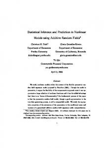
3. Prediction of risk of the terminal event Specific predictions can be obtained in the framework of joint modeling. Prediction consists of estimating the probability of an event at a given time t + w knowing the available information at prediction time t. Using a joint model, it is possible to estimate the probability of having the terminal event at time t+w given the history of the individual (occurrences of the recurrent events and/or the measurements of the longitudinal biomarker) prior to t. For the joint model for recurrent events and a terminal event (1), three settings of prediction were developed by Mauguen et al. (2013). In the first one, all the available information is accounted for, and we consider that this information is complete. In the second setting, all the known information is accounted for, however we consider that this information may be incomplete. Finally, in the third setting, recurrence information is not accounted for and only covariates are considered. All the settings are represented in Figure 1. Here, we focus on the first setting, for which we present the predictions and the accurate measures of predictive accuracy but in the package all the three setting are implemented for the joint models for recurrent and terminal events.

Agnieszka Król, Audrey Mauguen, Yassin Mazroui, Alexandre Laurent, Stefan Michiels, Virginie Rondeau 13

Setting 1

t

t+w

t

t+w

t

t+w

Exactly 2 recurrent events (x) before t Complete information

Setting 2 At least 2 recurrent events (x) before t Incomplete information

Setting 3 Whatever the history of recurrent events before t Observed recurrences history

Unobserved recurrences history

Window of prediction of death

Figure 1: Three settings to take into account patient history of recurrent events in prediction. Illustration with two recurrent events. For the joint models with a longitudinal outcome a complete history of the biomarker is considered (Kr´ ol et al. 2016). Thus, for Model (4) the individual’s history is the whole observed trajectory of the biomarker and for Model (5) it is the the whole observed trajectory of the biomarker and all the observed occurrences of the recurrent event (see Figure 2). The proposed prediction can be performed for patients from the population used to develop the model, but also for “new patients” from other populations. This is possible as the probabilities calculated are marginal, i.e., the conditional probabilities are integrated over the distribution of the random effects. Thus, values of patients frailties are not required to estimate the probabilities of the event. However, it should be noted that the predictions include individual deviations via the estimated parameters of the random effects’ distribution in a joint model. We denote by t the time at which the prediction is made and by w the window of prediction. Thus, we are interested in the probability of the event (death) at time t + w, knowing what happened before time t. The general formulation of predicted probability of the terminal event conditional on random effects and patient’s history is: Pi (t, t + w; ξ) = P (Ti∗ ≤ t + w|Ti∗ > t, Fi (t), X i ; ξ)

(8)

where X i are all the covariates included in the model, Fi (t) corresponds to the complete repeated data of patient i observed until time t. We define the complete history of recurrences J(l) R(l) (l)∗ (l)∗ Hi (t) = {Ni (t) = J (l) , Ti1 < · · · < TiJ ≤ t} (NiR (t) is the counting process of the recurrent events, l = 1, 2 for the two types of recurrent events, and in case of only one type of recurrent events in the models the index (l) is omitted) and the history of the biomarker Yi (t) = {yi (tiK ), ti1 < · · · < tiK < t}. Therefore, the individual’s history Fi (t) depends on the model considered and is equal to: Fi (t) = HiJ (t), for Model (1), (2) J(1) J(2) Fi (t) = {Hi (t), Hi (t)}, for Model (3) Fi (t) = Yi (t), for Model (4) J Fi (t) = {Hi (t), Yi (t)}, for Model (5) ∗ = 0 and T ∗ and for the recurrent events we assume Ti0 i(J+1) > t. For the estimated probabili-

14


Setting of complete history

Prediction

5 longitudinal measures (o) before t

of death t

Setting of complete history

t+w

Prediction

2 recurrent events (x) and 5 longitudinal measures (o) before t

of death

t

t+w

Figure 2: The possible prediction settings including the longitudinal data and considering the whole information available. The top setting correspond to the Model (4) and the bottom graphic to the Model (5). ties, confidence intervals are obtained by the Monte Carlo (MC) method, using the 2.5th and 97.5th percentiles of the obtained distribution (percentile confidence interval).

3.1. Brier score In order to validate the prediction ability of a given model, a prediction error is proposed using the weighted Brier score (Gerds and Schumacher 2006; Mauguen et al. 2013). It measures the distance between the prediction (probability of event) and the actual outcome (dead or alive). Inverse probability weighting corrects the score for the presence of right censoring. At a given horizon of prediction t + w, the error of prediction is calculated by: Errt+w =

Nt 1 X d [I(Ti∗ > t + w) − (1 − Pbi (t, t + w; b ξ))]2 w ci (t + w, G N) Nt

(9)

i=1

cn ) is defined by: where the weights w ci (t + w, G cn ) = w ci (t + w, G

I(Ti∗ ≤ t + w)δi I(Ti∗ > t + w) + , ∗ d d d d G G N (Ti )/GN (t) N (t + w)/GN (t)

d and G N (t) is the Kaplan-Meier estimate of the population censoring distribution at time t, Nt is the number of patients at risk of the event (alive and uncensored). Direct calculations of the Brier score are not implemented in the package frailtypack but using predictions Pbi (t, t + w; b ξ)), the Brier score can be obtained using weights w ci (·) function pec from the package pec (Gerds 2016) (for details, see the colorectal example in Section 5.3). For an internal validation (on a training dataset, i.e., used for estimation) of the model as a prediction tool for new patients, a k-fold cross-validation is used to correct for over-optimism. In this procedure, the joint model estimations are performed k times on k − 1 partitions from

Agnieszka Król, Audrey Mauguen, Yassin Mazroui, Alexandre Laurent, Stefan Michiels, Virginie Rondeau 15 the random split and the predictions are calculated on the left partitions. The prediction curves are based on these predictions, in the calculated for all the patients.

3.2. EPOCE Another method to evaluate a model’s predictive accuracy is the EPOCE estimator that is derived using prognostic conditional log-likelihood (Commenges et al. 2012). This measure is adapted both for an external data and then the Mean Prognosis Observed Loss (MPOL) is computed, as well as for the training data using the approximated Cross-Validated Prognosis Observed Loss (CVPOLa ). This measure of predictive accuracy is the risk function of an estimator of the true prognostic density function fT∗ |F (t),T ∗ ≥t , where F(t) denotes the history of repeated measurements and/or recurrent events until time t. Using information theory this risk is defined as the expectation of the loss function, that is the estimator derived from the joint model fT |F (t),T ∗ ≥t conditioned on T ∗ > t and this can be written as EPOCE(t) = E(−ln(fT |F (t),T ∗ >t )|T ∗ > t). In case of the model evaluated on the training data the approximated leave-one-out CVPOLa is defined by: CVPOLa (t) = −

Nt 1 X Fi (ξî , t) + N Trace(H −1 K t ), Nt

(10)

i=1

where H −1 is the inverted hessian matrix of the joint log-likelihood (Equation 6), K t = PN 1 i (ξ,t) ˆ > with v ˆ i = ∂li (Θ,ξ) |ˆ . The individual contribution îd ˆ i = ∂F∂ξ |ξˆ and d i i=1 I{Ti >t} v ∂ξ ξ Nt (N −1) to the log-likelihood of a terminal event at t defined for the individuals that are still at risk of the event at t can be written as:   l Y R (k) J(k) ˆ γL ˆ γR fT |u (Ti , δi |ui ; ξ)f ˆ u (ui ) dui   ui fYi (t)|ui (Yi (t)|ui ; ξ) fHJ(k) (t)|u (Hi (t)|ui ; ξ) i i i   i i   k=1 ˆ Fi (ξ, t) = ln  , l   R Y (k) J(k)  γ t ˆ R S (Ti |ui ; ξ)f ˆ u (ui ) dui  ˆ γL f J(k) (H (t)|ui ; ξ) fY (t)|u (Yi (t)|ui ; ξ) ui

i

i

k=1

Hi

(t)|ui

i

i

i

where Sit is the survival function of the terminal event for individual i. Again, l denotes the number of types of recurrent events included in the model. In case of the external data the MPOL(t) is expressed by the first component of the sum in the CVPOLa (t) (Equation 10). Indeed, the second component corresponds to the statistical risk introduced to the CVPOLa in order to correct for over-optimism coming from the use of the approximated cross-validation. The comparison of the models using the EPOCE can be done visually by tracking the 95% intervals of difference in EPOCE. The EPOCE estimator has some advantages comparing to the prediction error, in particular for the training data the approximated cross-validation technique is less computationally demanding than the crude leave-one-out cross-validation method for the prediction error, which is important in case of joint models when time of calculation is often long (ProustLima et al. 2014).

4. Modeling and prediction using the R package frailtypack

16


4.1. Estimation of joint models In the package frailtypack there are four different functions for the estimation of joint models, one for each model. The joint models for recurrent events and a terminal event (1) (and models for two clustered survival outcomes) as well as the general joint frailty models (2) are estimated with function frailtyPenal. The joint models for two recurrent events and a terminal event (3) are estimated with multivPenal. The estimation of joint models for a longitudinal outcome and a terminal event (4) is performed with longiPenal. Finally, function trivPenal estimates trivariate joint models (5). All these functions make calls to compiled Fortran codes programmed for computation and optimization of the log-likelihood. In the following, we detail each of the joint models functions. frailtyPenal function frailtyPenal(formula, formula.terminalEvent, data, recurrentAG = FALSE, cross.validation = FALSE, jointGeneral, n.knots, kappa, maxit = 300, hazard = "Splines", nb.int, RandDist = "Gamma", betaknots = 1, betaorder = 3, initialize = TRUE, init.B, init.Theta, init.Alpha, Alpha, init.Ksi, Ksi, init.Eta, LIMparam = 1e-3, LIMlogl = 1e-3, LIMderiv = 1e-3, print.times = TRUE) Argument formula is a two-sided formula for a survival object Surv from the survival package (Therneau and Lumley 2016) and it represents the recurrent event process (the first survival outcome for the joint models in case of clustered data) with the combination of covariates on the right-hand side, the indication of grouping variable (with term cluster(group)) and the indication of the variable for the terminal event (e.g., terminal(death)). It should be noted that the function cluster(x) is different from that included in the package survival. In both cases it is used for the identification of the correlated groups but in frailtypack it indicates the application of frailty model and in survival, a GEE (Generalized Estimating Equations) approach, without random effects. Argument formula.terminalEvent requires the combination of covariates related to the terminal event on the right-hand side. The name of data.frame with the variables used in the function should be put for argument data. Logical argument recurrentAG indicates whether the calendar timescale for recurrent events or clustered data with the counting process approach of Andersen and Gill (1982) (TRUE) or the gap timescale (FALSE by default) is to be used. Argument for the cross-validation cross.validation is not implemented for the joint models, thus its logical value must be FALSE. The smoothing parameters κ for a joint model can be chosen by first fitting suitable shared frailty and Cox models with the cross-validation method. The general joint frailty models (2) can be estimated if argument jointGeneral is TRUE. In this case, the additional gamma frailty term is assumed and the α parameter is not considered. These models can be applied only with the Gamma distribution for the random effects. The type of approximation of the baseline hazard functions is defined by argument hazard and can be chosen among Splines for semiparametric functions using equidistant intervals, Splines-per using percentile intervals, Piecewise-equi and Piecewise-per for piecewise constant functions using equidistant and percentile intervals, respectively and Weibull for the parametric Weibull baseline hazard functions. If Splines or Splines-per is chosen for the baseline hazard functions, arguments kappa for the positive smoothing parameters and n.knots should be given with the number of knots chosen between 4 and 20 which corresponds

Agnieszka Król, Audrey Mauguen, Yassin Mazroui, Alexandre Laurent, Stefan Michiels, Virginie Rondeau 17 to n.knots+2 splines functions for approximation of the baseline hazard functions (the same number for hazard functions for both outcomes). If Percentile-equi or Percentile-per is chosen for the approximation, argument nb.int should be given with a 2-element vector of numbers of time intervals (1-20) for the two baseline hazard functions of the model. Argument RandDist represents the type of the random effect distribution, either Gamma for the Gamma distribution or LogN for the normal distribution (log-normal joint model). If it is assumed that α in Model (1) is equal to zero, argument Alpha should be set to "None". In case of time dependent covariates, arguments betaknots and betaorder are used for the number of inner knots used for the estimation of B-splines (1, by default) and the order of B-splines (3 for quadratic B-splines, by default), respectively. The rest of the arguments are allocated for the optimization algorithm. Argument maxit declares the maximum number of iterations for the Marquardt algorithm. For a joint nested frailty model, i.e., a model that allow joint analysis of recurrent and terminal events for hierarchically clustered data, argument initialize determines whether the parameters should be initialized with estimated values from the appropriate nested frailty models. Arguments init.B, init.Theta, init.Eta and init.Alpha are vectors of initial values for regression coefficients, variances of the random effects and for the α parameter (by default, 0.5 is set for all the parameters). Arguments init.Ksi and Ksi are defined for joint nested frailty models and correspond to initial value for the flexibility parameter and the logical value indicating whether include this parameter in the model or not, respectively. The convergence thresholds of the Marquardt algorithm are for the difference between two consecutive log-likelihoods (LIMlogl), for the difference between the consecutive values of estimated coefficients (LIMparam) and for the small gradient of the log-likelihood (LIMderiv). All these threshold values are 10−3 by default. Finally, argument print.times indicates whether to print the iteration process (the information note about the calculation process and time taken by the program after terminating), the default is TRUE. The function frailtyPenal returns objects of class jointPenal if joint models are estimated. It should be noted that using this function univariate models: shared frailty models (Rondeau et al. 2012) and Cox models can be applied as well resulting with objects of class frailtyPenal. For both classes methods print(), summary() and plot() are available. multivPenal function multivPenal(formula, formula.Event2, formula.terminalEvent, data, initialize = TRUE, recurrentAG = FALSE, n.knots, kappa, maxit = 350, hazard = "Splines", nb.int, print.times = TRUE) This function allows to fit the multivariate frailty models (3). Argument formula must be a two-sided formula for a Surv object, corresponding to the first type of the recurrent event (no interval-censoring is allowed). Arguments formula.Event2 refer to the second type of the recurrent event and formula.terminalEvent to the terminal event, and are equal to linear combinations related to the respective events. The rest of the arguments is analogical to frailtyPenal. Arguments n.knots (values between 4 and 20) and kappa must be vectors of length 3 for each type of event, first for the recurrent event of type 1, second for the recurrent event of type 2 and third for the terminal event. The function multivPenal return objects of class multivPenal with print(), summary() and plot() methods available.

18


longiPenal function longiPenal(formula, formula.LongitudinalData, data, data.Longi, random, id, intercept = TRUE, link = "Random-effects", left.censoring = FALSE, n.knots, kappa, maxit = 350, hazard = "Splines", nb.int, init.B, init.Random, init.Eta, method.GH = "Standard", n.nodes, LIMparam = 1e-3, LIMlogl = 1e-3, LIMderiv = 1e-3, print.times = TRUE) In this function for the joint analysis of a terminal event and a longitudinal outcome, argument formula refers to the terminal event and the left-hand side of the formula must be a Surv object and the right-hand side, the explicative variables. Argument formula.LongitudinalData is equal to the sum of fixed explicative variables for the longitudinal outcome. For the model, two datasets are required: data containing information on the terminal event process and data.Longi with data related to longitudinal measurements. Random effects associated to the longitudinal outcome are defined with random using the appropriate names of the variables from data.Longi. If a random intercept is assumed, the option "1" should be used. For a random intercept and slope, arguments random should be equal to a vector with elements "1" and the name of a variable representing time point of the biomarker measurements. At the moment, more complicated structures of the random effects are not available in the package. The name of the variable representing the individuals in data.Longi is indicated by id. The logical argument intercept determines whether a fixed intercept should be included in the longitudinal part or not (default is TRUE). Two types of subject-specific link function are to choose and defined with the argument link. The default option "Random-effects" represents the link function of the random effects bi , otherwise the option is "Current-level" for the link function of the current level of the longitudinal outcome mi (t). The initial values of the estimated parameters can be indicated by init.B for the fixed covariates (a vector of values starting with the parameters associated to the terminal event and then for the longitudinal outcome, interactions in the end of each component), init.Random for the vector of elements of the Cholesky decomposition of the covariance matrix of the random effects ui and init.Eta for the regression coefficients associated to the link function. There are three methods of the Gaussian quadrature to approximate the integrals to choose from. The default Standard corresponds to the non-adaptive Gauss-Hermite quadrature for multidimensional integrals. The other possibility is the pseudo-adaptive Gaussian quadrature ("Pseudo-adaptive") (Rizopoulos 2012). Finally, the multivariate non-adaptive Gaussian quadrature using the algorithm implemented in a Fortran subroutine HRMSYM is indicated by "HRMSYM" (Genz and Keister 1996). The number of the quadrature nodes (n.nodes) can be chosen among 5, 7, 9, 12, 15, 20 and 32 using argument (default is 9). The function longiPenal return objects of class longiPenal with print(), summary() and plot() methods available. trivPenal function trivPenal(formula, formula.terminalEvent, formula.LongitudinalData, data, data.Longi, random, id, intercept = TRUE, link = "Random-effects", left.censoring = FALSE, recurrentAG = FALSE, n.knots, kappa, maxit = 300, hazard = "Splines", nb.int, init.B, init.Random, init.Eta, init.Alpha, method.GH = "Standard", n.nodes, LIMparam = 1e-3, LIMlogl = 1e-3, LIMderiv = 1e-3, print.times = TRUE)

Agnieszka Król, Audrey Mauguen, Yassin Mazroui, Alexandre Laurent, Stefan Michiels, Virginie Rondeau 19 The function for the trivariate joint model comprises three formulas for each type of process. The first two arguments are analogous to frailtyPenal, argument formula, referring to recurrent events, is a two-sided formula for a Surv object on the left-hand side and covariates on the right-hand side (with indication of the variable for the terminal event using method terminal) and argument formula.terminalEvent represents the terminal event and is equal to a linear combination of the explicative variables. Finally, argument formula.LongitudinalData as in function longiPenal corresponds to the longitudinal outcome indicating the fixed effect covariates. The rest of the arguments are detailed in the descriptions of functions frailtyPenal and longiPenal. The function trivPenal return objects of class trivPenal with print(), summary() and plot() methods available.

4.2. Prediction The current increase of interest in the joint modeling of correlated data is often related to the individual predictions that these models offer. Indeed, calculating the probabilities of a terminal event given a joint model results in precise predictions that consider the past of an individual. Moreover, there exist statistical tools that evaluate a model’s capacity for these dynamic predictions. In the package frailtypack we provide prediction function for dynamic predictions of a terminal event in a finite horizon, epoce function for evaluating predictive accuracy of a joint model and Diffepoce for comparing the accuracy of two joint models. Predicted probabilities with prediction function In the package it is possible to calculate the prediction probabilities for the Cox proportional hazard, shared frailty (for clustered data, Rondeau et al. (2012)) and joint models. Among the joint models the predictions are provided for the standard joint frailty models (recurrent events and a terminal event), for the joint models for a longitudinal outcome and a terminal event and for the trivariate joint models (a longitudinal outcome, recurrent events and a terminal event). These probabilities can be calculated for a given prediction time and a window or for a vector of times, with varying prediction time or varying window. For the shared frailty models for clustered events, marginal and conditional on a specific cluster predictions can be calculated and for the joint models only the marginal predictions are provided. Finally, for the joint frailty models the predictions are calculated in three settings: given the exact history of recurrences, given the partial history of recurrences (the first J recurrences) and ignoring the past recurrences. For the joint models with a longitudinal outcome (bivariate and trivariate) only the predictions considering the patient’s complete history are provided. For all the aforementioned predictions the following function is proposed: prediction(fit, data, data.Longi, t, window, group, MC.sample = 0) Argument fit indicates the, a frailtyPenal, jointPenal, longiPenal or trivPenal object. The data with individual characteristics for predictions must be provided in dataframe data with information on the recurrent events and covariates related to recurrences and the terminal event and in case of longiPenal and trivPenal dataframe data.Longi containing repeated measurements and covariates related to the longitudinal outcome. These two datasets must refer to the same individuals for which the predictions will be calculated. Moreover, the names and the types of variables should be equivalent to those in the dataset used for estimation. The details on how to prepare correctly the data are presented in appropriate examples (Section 5).

20


Argument t is a time or vector of times for predictions and window is a horizon or vector of horizons. The function calculates the probability of the terminal event between a time of prediction and a horizon (both arguments are scalars), between several times of prediction and a horizon (t is a vector and window a scalar) and finally, between a time of prediction and several horizons (t is a scalar and window a vector of positive values). For all the predictions, confidence intervals can be calculated using the MC method with MC.sample number of samples (maximum 1000). If the confidence bands are not to be calculated argument MC.sample should be equal to 0 (the default). Predictive accuracy measure with epoce and Diffepoce functions Predictive ability of joint models can be evaluated with function epoce that computes the estimators of the EPOCE, the MPOL and CVPOLa . For a given estimation, the evaluation can be performed on the same data and then both MPOL and CVPOLa are calculated, as well as on a new dataset but then only MPOL is calculated as the correction for over-optimism is not necessary. The call of the function is: epoce(fit, pred.times, newdata = NULL, newdata.Longi = NULL) with fit an object of jointPenal, longiPenal or trivPenal classes, pred.times a vector of time for which the calculations are performed. In case of external validation, new datasets newdata and newdata.Longi should be provided (newdata.Longi only in case of longiPenal and trivPenal objects). However, the names and types of variables in newdata and newdata.Longi must be the same as in the datasets used for estimation. To compare the predictive accuracy of two joint models fit to the same data but possibly with different covariates, the simple comparison of obtained values of EPOCE can be enhanced by calculating the 95% tracking interval of difference between the EPOCE estimators. For this purpose we propose function: Diffepoce(epoce1, epoce2) where epoce1 and epoce2 are objects inheriting from the epoce class.

5. Illustrating examples The package frailtypack provides various functions for models for correlated outcomes and survival data. The Cox proportional hazard model, the shared frailty model for recurrent events (clustered data), the nested frailty model, the additive frailty model and the joint frailty model for recurrent events and a terminal event have already been illustrated elsewhere (Rondeau and Gonzalez 2005; Rondeau et al. 2012). In this section we focus on extended models for correlated data presented in Section 2 using three datasets: readmission, dataMultiv and colorectal. Although the joint frailty model has already been presented in the literature, we illustrate its usage as the form of the function has developed in the meantime.

5.1. Example on dataset readmission for joint frailty models

Agnieszka Król, Audrey Mauguen, Yassin Mazroui, Alexandre Laurent, Stefan Michiels, Virginie Rondeau 21 Dataset readmission comes from a rehospitalization study of patients after a surgery and diagnosed with colorectal cancer (Gonzalez, Fernandez, Moreno, Ribes, Merce, Navarro, Cambray, and Borras 2005; Rondeau et al. 2012). It contains information on times (in days) of successive hospitalizations and death (or last registered time of follow-up for right-censored patients) counting from date of surgery, and patients characteristics: type of treatment, sex, Dukes’ tumoral stage, comorbidity Charlson’s index and survival status. The dataset includes 403 patients with 861 rehospitalization events in total. Among the patients 112 (28%) died during the study.

Standard joint frailty model We adapt the joint model for recurrent events and a terminal event using the gap timescale from the example given in (Rondeau et al. 2012). The model modJoint.gap is defined: R> library("frailtypack") R> data("readmission") R> modJoint.gap plot(aggregate(readmission$t.stop, by = list(readmission$id), + FUN = max)[2][ ,1], modJoint.gap$martingale.res, ylab = "", + xlab = "time", main = "Rehospitalizations", ylim = c(-4, 4)) R> lines(lowess(aggregate(readmission$t.stop, by = list(readmission$id), + FUN = max)[2][ ,1], modJoint.gap$martingale.res, f = 1), lwd = 3, + col = "grey")

22


R> plot(aggregate(readmission$t.stop, by = list(readmission$id), + FUN = max)[2][ ,1], modJoint.gap$martingaledeath.res, ylab = "", + xlab = "time", main = "Death", ylim = c(-2, 2)) R> lines(lowess(aggregate(readmission$t.stop, by = list(readmission$id), + FUN = max)[2][ ,1], modJoint.gap$martingaledeath.res, f = 1), lwd = 3, + col = "grey") ●

Rehospitalizations

Death

●

2

4

●

1

● ● ● ●●● ●● ● ● ●● ● ●●● ● ● ●● ● ●● ● ● ● ● ● ● ● ●● ●● ● ● ●● ● ● ● ● ● ● ●● ● ●● ● ● ● ● ●●● ●● ● ● ● ● ●● ● ●● ● ● ● ●●● ● ● ● ● ● ●● ● ● ● ●● ● ● ● ● ● ● ● ● ●● ● ●● ● ●● ● ● ● ● ●● ● ● ● ● ● ● ●● ● ● ● ● ●● ●● ●● ●● ● ● ● ●● ● ● ● ● ● ● ● ● ● ● ● ● ● ● ● ● ● ● ● ● ● ● ● ● ● ● ● ● ● ● ● ● ●● ● ● ● ● ● ● ●●● ● ● ● ● ● ● ● ● ● ● ● ● ● ●● ● ● ●● ● ● ● ● ● ● ● ● ● ● ● ● ● ● ● ● ● ● ● ●● ● ● ● ● ● ● ● ● ● ●● ● ● ● ● ●● ●● ● ● ● ● ●● ● ●●●●● ● ● ●● ● ●●● ●● ●● ● ●● ●● ● ● ● ● ●● ● ●● ● ● ●● ● ● ● ● ●● ● ● ●

−1

0

● ● ● ●● ● ● ● ● ● ● ● ● ● ● ●●● ● ●● ● ● ● ● ● ● ● ● ● ●● ● ● ● ● ● ● ● ●● ● ● ●●● ● ● ●● ● ● ● ● ● ● ●● ●●●●●● ●● ●● ● ● ● ● ● ● ● ●●● ●●● ● ●●●● ● ● ●●●● ●●● ● ●● ●● ● ● ● ●● ●●● ●●● ● ●●● ●● ● ●● ● ● ● ● ● ● ●● ●● ●● ● ● ●● ●● ●● ●● ● ●● ● ● ● ●●●● ● ● ●●● ● ●● ● ●● ●● ● ● ● ● ● ● ● ●●● ● ●●●● ● ● ● ● ● ● ● ●●●● ● ● ● ● ● ● ● ● ● ● ● ● ● ● ● ● ● ● ● ● ●●● ● ● ● ● ● ● ● ● ● ● ● ● ● ● ● ● ● ● ● ● ● ● ● ● ● ● ● ● ● ● ● ● ● ● ● ● ● ● ● ● ● ● ● ● ● ● ● ●● ● ● ● ● ● ● ● ● ● ● ● ● ● ● ● ● ● ●● ● ●● ●● ● ● ● ● ● ● ● ● ● ● ● ● ● ● ● ● ● ● ● ●●

−2

0

2

● ● ●

● ● ●

●

−2

−4

● ● ●

0

500

1000

1500

2000

0

500

1000

●

1500

2000

●

time

time

Figure 3: Martingale residuals for rehospitalizations and death against the follow-up time (in days). The grey line corresponds to a smooth curve obtained with lowess. For the rehospitalization process the mean of residuals was approximately 0 with the smooth curve close to the line y = 0, but in case of death this tendency was deviated by relatively higher values for short follow-up times. This may suggest, that the model may have underestimated the number of death in the early follow-up period. The identified individuals of which the residuals result in non-zero mean, had short intervals between their rehospitalization and death (1 day). Indeed, the removal of these individuals (50 patients) resulted in residuals with the mean close to 0 all along the follow-up period (plot not shown here). The package frailtypack provides also the estimation of the random effects. Vector frailty.pred from jointPenal object contains the individual empirical Bayes estimates. They can be graphically represented for each individual with additional information on number of events (point size) to identify the outlying data. R> plot(1 : 403, modJoint.gap$frailty.pred, xlab = "Id of patients", + ylab = "Frailty predictions for each patient", type = "p", axes = F, + cex = as.vector(table(readmission$id)), pch = 1, ylim = c(-0.1, 7), + xlim = c(-2, 420)) R> axis(1, round(seq(0, 403, length = 10), digit = 0)) R> axis(2, round(seq(0, 7, length = 10), digit = 1)) Figure 4 shows the values of frailty prediction for each patient with an association to the number of events (the bigger the point, the greater the number of rehospitalizations). The

Agnieszka Król, Audrey Mauguen, Yassin Mazroui, Alexandre Laurent, Stefan Michiels, Virginie Rondeau 23

6.2 4.7 3.1 1.6 0.0

Frailty predictions for each patient

frailties tended to have bigger values if the number of events of a given individual was high. From the plot it can be noticed that there was an outlying frailty suggesting verification of the follow-up of the concerned individual.

●

●

● ●●● ● ● ●●●● ●● ●● ● ●● ● ● ●● ● ●● ● ●●● ●●● ● ● ● ● ● ● ●● ● ● ●● ● ●●●● ● ● ●● ● ● ●● ● ● ● ● ●●● ●●● ●● ● ● ● ● ● ● ●● ● ● ● ● ● ● ● ● ● ● ● ● ● ● ●● ●● ● ●● ● ● ● ● ● ● ● ● ● ● ● ● ● ● ● ● ● ● ● ● ● ● ● ● ● ● ● ● ● ● ● ● ● ● ● ● ● ● ●● ● ●● ● ● ●● ● ● ● ● ● ● ● ● ● ●●● ● ● ● ● ● ● ● ● ●● ● ● ● ● ● ● ● ● ● ● ● ● ● ● ● ● ● ● ● ● ● ● ● ● ● ● ● ● ● ● ● ● ● ● ● ● ● ● ● ● ● ● ● ● ● ● ● ● ● ● ● ● ● ● ● ● ● ● ● ● ● ● ● ● ● ● ● ● ● ●● ● ● ● ● ● ● ●●● ● ●● ●● ● ●●●● ● ●● ● ● ● ●● ● ● ● ● ● ●●● ● ● ● ● ●● ●● ● ●● ●● ●● ● ● ● ● ● ●●●● ● ●●● ● ● ● ●● ● ● ● ● ●● ● ●● ● ●● ●● ● ● ● ●● ● ●● ● ● ●●● ● ●● ● 0

45

90

134

179

224

269

313

358

403

Id of patients

Figure 4: Individual prediction of the frailties. The size of points corresponds to number of an individual’s recurrent events.

Time-varying coefficients In the framework of standard joint frailty models, it is possible to fit the models with timevarying effects of prognostic factors. Using function timedep in a formula of frailtyPenal, the time-dependent coefficients can be estimated using B-splines of order q (option betaorder) with m interior knots (option betaknots). In the example of readmission dataset we are interested in verifying whether the variable sex has a time-varying effect on both recurrent and terminal events. Thus, we fit a model equivalent to modJoint.gap but with time dependent effects assuming quadratic B-splines and 3 interior knots: R> modJoint.gap.timedep 0). For death, at the beginning, the effect of sex was weakening the risk but shortly became non-influential (β(t) around 0). The PH assumption for the variable sex can be checked using the LR test. We compare two models: modJoint.gap (related to the null hypothesis that the effect is constant in time: H0 : βR (t) = βR , βT (t) = βT ) and modJoint.gap.timedep (related to the alternative hypothesis of time-varying effects is time-varying: H1 : βR (t) 6= βR , βT (t) 6= βT ):

24


R> LR.statistic p.value modJoint.gap.nosex LR.statistic p.value + R> R> R> R> R>

datapred 69 years 0 No

30


6 7 8 9 10

2 2 2 2 2

0.1639344 0.2814208 0.4316940 0.5846995 0.7377049

1.3919052 1.2063562 1.2063562 0.9462067 1.9353985

C C C C C

>69 >69 >69 >69 >69

years years years years years

0 0 0 0 0

No No No No No

R> data("colorectal") R> head(colorectal, 5)

1 2 3 4 5 1 2 3 4 5

id time0 time1 new.lesions treatment age who.PS 1 0.0000000 0.7095890 0 S 60-69 years 0 2 0.0000000 1.2821918 0 C >69 years 0 3 0.0000000 0.5245902 1 S 60-69 years 1 3 0.5245902 0.9207650 1 S 60-69 years 1 3 0.9207650 0.9424658 0 S 60-69 years 1 prev.resection state gap.time No 1 0.70958904 No 1 1.28219178 No 0 0.52459017 No 0 0.39617486 No 1 0.02170073

Joint model for longitudinal data and a terminal event Firstly, we estimated the bivariate joint model for longitudinal data and a terminal event (4). We considered a left-censored biomarker, transformed tumor size measurements are not observed below a threshold -3.33 (which corresponds to ’zero’ measures in the nontransformed data). The value of κ smoothing parameter was chosen using a corresponding reduced model, ie. a Cox model for the terminal event. For a model with a random intercept and slope for the biomarker and the link function being the random effects of the biomarker we used the following form of the longiPenal function using colorectalLongi dataset and a subset colorectal with only information on the terminal event (colorectalSurv): R> colorectalSurv modLongi modLongi > modLongi Call: longiPenal(formula = Surv(time1, state) ~ age + treatment + who.PS + prev.resection, formula.LongitudinalData = tumor.size ~ year * treatment + age + who.PS, data = colorectalSurv, data.Longi = colorectalLongi,

Agnieszka Król, Audrey Mauguen, Yassin Mazroui, Alexandre Laurent, Stefan Michiels, Virginie Rondeau 31 random = c("1", "year"), id = "id", link = "Random-effects", left.censoring = -3.33, n.knots = 8, kappa = 0.93, method.GH = "Pseudo-adaptive", n.nodes = 7) Joint Model for Longitudinal Data and a Terminal Event Parameter estimates using a Penalized Likelihood on the hazard function and assuming left-censored longitudinal outcome Association function: random effects Longitudinal outcome: ---------------coef SE coef (H) SE coef (HIH) Intercept 3.023259 0.187384 0.187384 year -0.303105 0.135847 0.135847 treatmentC 0.048720 0.213961 0.213961 age60-69 years -0.017015 0.168804 0.168804 age>69 years -0.294597 0.131867 0.131867 who.PS1 0.106983 0.116952 0.116952 who.PS2 0.739941 0.175652 0.175652 year:treatmentC -0.634663 0.183640 0.183640

z 16.134028 -2.231218 0.227703 -0.100797 -2.234047 0.914761 4.212540 -3.456020

p 69 years treatmentC who.PS1 who.PS2 prev.resectionYes

coef exp(coef) SE coef (H) SE coef (HIH) -0.226281 0.797494 0.243004 0.243004 -0.100922 0.904004 0.223801 0.223801 -0.090385 0.913580 0.198843 0.198843 -0.116794 0.889769 0.218352 0.218352 0.802399 2.230887 0.258302 0.258302 -0.225774 0.797898 0.193418 0.193418

p 3.5176e-01 6.5203e-01 6.4943e-01 5.9273e-01 1.8936e-03 2.4309e-01 chisq df global p age 1.07045 2 0.58600 who.PS 9.93603 2 0.00696

z -0.931181 -0.450944 -0.454554 -0.534889 3.106433 -1.167288

32


Components of Random-effects covariance matrix B1: Intercept 1.972030 -0.519742 year -0.519742 0.943568 Association parameters: coef SE z p Intercept 0.3203431 0.0848202 3.77673 0.0001589 year 0.0432288 0.1668875 0.25903 0.7956100 Residual standard error:

0.954237

(SE (H):

0.027079 )

penalized marginal log-likelihood = -1684.01 Convergence criteria: parameters = 0.000127 likelihood = 0.000361 gradient = 1.47e-08 LCV = the approximate likelihood cross-validation criterion in the semi parametrical case = 1.62312 n= 150 n repeated measurements= 906 Percentage of left-censored measurements= 3.75 % Censoring threshold s= -3.33 n events= 121 number of iterations: 26 Exact number of knots used: 8 Value of the smoothing parameter: 0.93 Gaussian quadrature method: Pseudo-adaptive with 7 nodes On average, the tumor size significantly decreased in time in interaction with the treatment, this effect was more important in the C arm (-0.63, p-value = 0.001). However, there was no effect of treatment arm on the risk of death (HR = 0.91, p-value = 0.65). The age of patients at baseline did not have any effect neither on the tumor size nor on the risk of death. The performance status WHO 2 evaluated before the treatment was a prognostic factor both for the tumor size (0.74, p-value plot(modLongi, main = "Hazard function")

Agnieszka Król, Audrey Mauguen, Yassin Mazroui, Alexandre Laurent, Stefan Michiels, Virginie Rondeau 33 R> + + R> + + R> + R> R> + +

plot(aggregate(colorectalSurv$time1, by = list(colorectalSurv$id), FUN = max)[2][ ,1], modLongi$martingaledeath.res, ylab = "", xlab = "time", main = "Martingale Residuals - Death", ylim = c(-4.2, 4.2)) lines(lowess(aggregate(colorectalSurv$time1, by = list(colorectalSurv$id), FUN = max)[2][ ,1], modLongi$martingaledeath.res, f = 1), lwd = 3, col = "grey") qqnorm(modLongi$marginal_chol.res, main = "Marginal Cholesky residuals", xlab = "") qqline(modLongi$marginal_chol.res) plot(modLongi$pred.y.cond, modLongi$conditional.res, xlab = "Fitted", ylab = "Conditional residuals", main = "Conditional Residuals vs. Fitted Values")

Next, we explored predictiveness of this model comparing it with a model in which the link function was represented by the current level of the biomarker mi (t). Thus, we fitted a bivariate model with the same covariates and characteristics but with the option link = "Current-level" (model modLongi2). Then, for times of prediction between 1.2 and 2.5 years we calculated the EPOCE estimator. We compared the models by plotting values of CVPOLa and tracking intervals for the differences between the models. R> + + + + R> R> R> R> R> + R> R> + R>

modLongi2 + + R> + + R> + R> R> + +

plot(modTrivariate, main = "Hazard functions") plot(modTrivariate, type = "Survival", main = "Survival functions") plot(aggregate(colorectal$time1, by = list(colorectal$id), FUN = max)[2][ ,1], modTrivariate$martingaledeath.res, ylab = "", xlab = "time", main = "Martingale Residuals - Death", ylim = c(-4.2, 4.2)) lines(lowess(aggregate(colorectal$time1, by = list(colorectal$id), FUN = max)[2][ ,1], modTrivariate$martingaledeath.res, f = 1), lwd = 3, col = "grey") plot(aggregate(colorectal$time1, by = list(colorectal$id), FUN = max)[2][ ,1], modTrivariate$martingale.res, ylab = "", xlab = "time", main = "Martingale Residuals\n - Recurrences", ylim = c(-4.2, 4.2)) lines(lowess(aggregate(colorectal$time1, by = list(colorectal$id), FUN = max)[2][ ,1], modTrivariate$martingale.res, f = 1), lwd = 3, col = "grey") qqnorm(modTrivariate$marginal_chol.res, main = "Marginal Cholesky residuals" ,xlab = "") qqline(modTrivariate$marginal_chol.res) plot(modTrivariate$pred.y.cond, modTrivariate$conditional.res, xlab = "Fitted", ylab = "Conditional residuals", main = "Conditional Residuals \n vs. Fitted Values")

The martingale residuals for both recurrences and death processes showed slight signs of skewness, their means seemed to decrease in time. Using the marginal Cholesky residuals and the conditional residuals we found that the model did not fit the longitudinal data very well. We compared the trivariate model modTrivariate with the bivariate model modLongi in terms of predictive accuracy for OS using the Brier Score. Firstly, we defined the prediction time and horizons and calculated the predictions for the bivariate and trivariate models:

Agnieszka Król, Audrey Mauguen, Yassin Mazroui, Alexandre Laurent, Stefan Michiels, Virginie Rondeau 39 R> R> R> R> + R> +

predtime R> + R>

data_surv + + + R> + + R> + R> + R> R> R>

library("pec") library("prodlim") source("/ipcw_2-9_modif.R") source("/pecMethods_2-9_modif.R") BrierScore = predtime, ], cens.model = "marginal", data.cens = data_surv, exact = FALSE, times = fwindow, ptime = predtime, reference = FALSE) plot(fwindow, BrierScore$AppErr$Bivariate[-1], pch = 6, main = "", ylab = "Prediction error", xlab = "Years", ylim = c(0, 0.3), xlim = c(0.9, 2.7), col = "black", type = "l", lwd = 2, axes = F, lty = 1) points(fwindow, BrierScore$AppErr$Trivairate[-1], pch = 15, col = "blue", type = "l", lwd = 2, lty = 2) legend(2.1, 0.3, legend = c("modLongi", "modTrivariate"), bty = "n", cex = 1.1, lty = c(1, 2), lwd = 2, col = c("black", "blue")) axis(1, at = seq(0.9, 2.7, by = 0.3)) axis(2, at = seq(0, 0.3, by = 0.1)) abline(v = 1, lty = 2, lwd = 2, col = "gray35")

Figure 7 represents the prediction error curves for both models. In short prediction horizons, values of the Brier Score of the models were very close to each other. After around 1.6 years the bivariate model had better predictive accuracy than the trivariate model. However, the


0.3

40

0.0

0.1

Prediction error

0.2

modLongi modTrivariate

0.9

1.2

1.5

1.8

2.1

2.4

2.7

Years

Figure 7: Error of prediction at t = 1 year and varying window w from 0.1 to 1.5. modLongi - tumor size and death, modTrivariate - tumor size, occurrence of new lesions and death.

results are presented for the apparent error calculated using the data from the estimation. For verification of the models for predictions for new patients (not used in the data for the estimation) a cross-validation procedure would be required.

Dynamic Predictions Both, for the bivariate models for longitudinal data and a terminal event and for the trivariate models, the package provides individual predictions of the terminal event. To create patients’ profiles, two datasets must be provided, one including the history of the biomarker and the values of covariates at measurement times (dataLongi) and a second one with the information on covariates related to the terminal event (data). In case of the trivariate model, this dataset should also include the history of recurrences. For the example of colorectal dataset, we created two profiles of patients that differed from each other by the trajectory of the tumor size. The first patient had a progressive disease with a tumor size increasing in time and the second patient a response to the treatment with a diminishing tumor. Both patients had the same baseline characteristics. In the step of creating the data, types of variables must be appropriate and coherent with the dataset used for estimation. Firstly, we prepared the data for the bivariate model setting: R> + R> + R> R>

datapredj_longi R>

datapredj_longi[1, datapredj_longi[2, datapredj_longi[3, datapredj_longi[4, datapredj_longi[5,

] ] ] ] ]

datapredj_longi[6,] R> R>

datapredj R> R>

datapredj

Tutorial in Joint Modeling and Prediction: a statistical software ... - arXiv

Tutorial in Joint Modeling and Prediction: a statistical software ... - arXiv

Suggest Documents