TUTORIAL No. 1 FLUID FLOW THEORY In order to ...

TUTORIAL No. 1 FLUID FLOW THEORY In order to complete this tutorial you should already have completed level 1 or have a good basic knowledge of fluid mechanics equivalent to the Engineering Council part 1 examination 103.

When you have completed this tutorial, you should be able to do the following. ‰

Explain the meaning of viscosity.

‰

Define the units of viscosity.

‰

Describe the basic principles of viscometers.

‰

Describe non-Newtonian flow

‰

Explain and solve problems involving laminar flow though pipes and between parallel surfaces.

‰

Explain and solve problems involving drag force on spheres.

‰

Explain and solve problems involving turbulent flow.

‰

Explain and solve problems involving friction coefficient.

Throughout there are worked examples, assignments and typical exam questions. You should complete each assignment in order so that you progress from one level of knowledge to another. Let us start by examining the meaning of viscosity and how it is measured.

© D.J.DUNN

1

1. VISCOSITY 1.1 BASIC THEORY Molecules of fluids exert forces of attraction on each other. In liquids this is strong enough to keep the mass together but not strong enough to keep it rigid. In gases these forces are very weak and cannot hold the mass together. When a fluid flows over a surface, the layer next to the surface may become attached to it (it wets the surface). The layers of fluid above the surface are moving so there must be shearing taking place between the layers of the fluid.

Fig.1.1 Let us suppose that the fluid is flowing over a flat surface in laminated layers from left to right as shown in figure 1.1. y is the distance above the solid surface (no slip surface) L is an arbitrary distance from a point upstream. dy is the thickness of each layer.

dL is the length of the layer. dx is the distance moved by each layer relative to the one below in a corresponding time dt. u is the velocity of any layer. du is the increase in velocity between two adjacent layers. Each layer moves a distance dx in time dt relative to the layer below it. The ratio dx/dt must be the change in velocity between layers so du = dx/dt. When any material is deformed sideways by a (shear) force acting in the same direction, a shear stress τ is produced between the layers and a corresponding shear strain γ is produced. Shear strain is defined as follows.

γ=

sideways deformation dx = height of the layer being deformed dy

The rate of shear strain is defined as follows.

γ& =

shear strain γ dx du = = = time taken dt dt dy dy

It is found that fluids such as water, oil and air, behave in such a manner that the shear stress between layers is directly proportional to the rate of shear strain.

τ = constant x γ& Fluids that obey this law are called NEWTONIAN FLUIDS. © D.J.DUNN

2

It is the constant in this formula that we know as the dynamic viscosity of the fluid. DYNAMIC VISCOSITY µ =

shear stress dy τ = =τ rate of shear γ& du

FORCE BALANCE AND VELOCITY DISTRIBUTION A shear stress τ exists between each layer and this increases by dτ over each layer. The pressure difference between the downstream end and the upstream end is dp. The pressure change is needed to overcome the shear stress. The total force on a layer must be zero so balancing forces on one layer (assumed 1 m wide) we get the following.

dp dy + dτ dL = 0 dτ dp =− dy dL It is normally assumed that the pressure declines uniformly with distance downstream so the pressure gradient

dp is assumed constant. The minus sign indicates that the pressure falls with distance. dL

Integrating between the no slip surface (y = 0) and any height y we get

⎛ du ⎞ d ⎜⎜ µ ⎟⎟ dy ⎠ dp dτ − = = ⎝ dy dL dy −

dp d 2u = µ 2 ..............(1.1) dL dy

Integrating twice to solve u we get the following.

−y

dp du =µ +A dL dy

y 2 dp − = µu + Ay + B 2 dL A and B are constants of integration that should be solved based on the known conditions (boundary conditions). For the flat surface considered in figure 1.1 one boundary condition is that u = 0 when y = 0 (the no slip surface). Substitution reveals the following. 0 = 0 +0 +B hence B = 0 At some height δ above the surface, the velocity will reach the mainstream velocity uo. This gives us the second boundary condition u = uo when y = δ.

© D.J.DUNN

3

Substituting we find the following.

δ 2 dp = µu o + Aδ 2 dL δ dp µu o A=− hence − 2 dL δ y 2 dp ⎛ δ dp µu o ⎞ − = µu + ⎜ − − ⎟y 2 dL δ ⎠ ⎝ 2 dL ⎛ δ dp u o ⎞ ⎟⎟ + u = y⎜⎜ ⎝ 2µ dL δ ⎠

−

Plotting u against y gives figure 1.2. BOUNDARY LAYER.

The velocity grows from zero at the surface to a maximum at height δ. In theory, the value of δ is infinity but in practice it is taken as the height needed to obtain 99% of the mainstream velocity. This layer is called the boundary layer and δ is the boundary layer thickness. It is a very important concept and is discussed more fully in later work. The inverse gradient of the boundary layer is du/dy and this is the rate of shear strain γ.

Fig.1.2

© D.J.DUNN

4

1.2. UNITS of VISCOSITY 1.2.1 DYNAMIC VISCOSITY µ

The units of dynamic viscosity µ are N s/m2. It is normal in the international system (SI) to give a name to a compound unit. The old metric unit was a dyne.s/cm2 and this was called a POISE after Poiseuille. The SI unit is related to the Poise as follows. 10 Poise = 1 Ns/m2 which is not an acceptable multiple. Since, however, 1 Centi Poise (1cP) is 0.001 N s/m2 then the cP is the accepted SI unit. 1cP = 0.001 N s/m2.

The symbol η is also commonly used for dynamic viscosity. There are other ways of expressing viscosity and this is covered next. 1.2.2 KINEMATIC VISCOSITY ν

This is defined as : ν = dynamic viscosity /density ν = µ/ρ

The basic units are m2/s. The old metric unit was the cm2/s and this was called the STOKE after the British scientist. The SI unit is related to the Stoke as follows. 1 Stoke (St) = 0.0001 m2/s and is not an acceptable SI multiple. The centi Stoke (cSt),however, is 0.000001 m2/s and this is an acceptable multiple. 1cSt = 0.000001 m2/s = 1 mm2/s 1.2.3 OTHER UNITS

Other units of viscosity have come about because of the way viscosity is measured. For example REDWOOD SECONDS comes from the name of the Redwood viscometer. Other units are Engler Degrees, SAE numbers and so on. Conversion charts and formulae are available to convert them into useable engineering or SI units. 1.2.4 VISCOMETERS

The measurement of viscosity is a large and complicated subject. The principles rely on the resistance to flow or the resistance to motion through a fluid. Many of these are covered in British Standards 188. The following is a brief description of some types.

© D.J.DUNN

5

U TUBE VISCOMETER The fluid is drawn up into a reservoir and allowed to run through a capillary tube to another reservoir in the other limb of the U tube. The time taken for the level to fall between the marks is converted into cSt by multiplying the time by the viscometer constant. ν = ct The constant c should be accurately obtained by calibrating the viscometer against a master viscometer from a standards laboratory. Fig.1.3 REDWOOD VISCOMETER This works on the principle of allowing the fluid to run through an orifice of very accurate size in an agate block. 50 ml of fluid are allowed to fall from the level indicator into a measuring flask. The time taken is the viscosity in Redwood seconds. There are two sizes giving Redwood No.1 or No.2 seconds. These units are converted into engineering units with tables.

Fig.1.4

© D.J.DUNN

6

FALLING SPHERE VISCOMETER This viscometer is covered in BS188 and is based on measuring the time for a small sphere to fall in a viscous fluid from one level to another. The buoyant weight of the sphere is balanced by the fluid resistance and the sphere falls with a constant velocity. The theory is based on Stokes’ Law and is only valid for very slow velocities. The theory is covered later in the section on laminar flow where it is shown that the terminal velocity (u) of the sphere is related to the dynamic viscosity (µ) and the density of the fluid and sphere (ρf and ρs) by the formula Fig.1.5

µ = F gd2(ρs -ρf)/18u

F is a correction factor called the Faxen correction factor, which takes into account a reduction in the velocity due to the effect of the fluid being constrained to flow between the wall of the tube and the sphere. ROTATIONAL TYPES There are many types of viscometers, which use the principle that it requires a torque to rotate or oscillate a disc or cylinder in a fluid. The torque is related to the viscosity. Modern instruments consist of a small electric motor, which spins a disc or cylinder in the fluid. The torsion of the connecting shaft is measured and processed into a digital readout of the viscosity in engineering units. You should now find out more details about viscometers by reading BS188, suitable textbooks or literature from oil companies.

ASSIGNMENT No. 1

1.

Describe the principle of operation of the following types of viscometers.

a.

Redwood Viscometers.

b.

British Standard 188 glass U tube viscometer.

c.

British Standard 188 Falling Sphere Viscometer.

d.

Any form of Rotational Viscometer

Note that this covers the E.C. exam question 6a from the 1987 paper.

© D.J.DUNN

7

2. LAMINAR FLOW THEORY

The following work only applies to Newtonian fluids. 2.1 LAMINAR FLOW A stream line is an imaginary line with no flow normal to it, only along it. When the flow is laminar, the streamlines are parallel and for flow between two parallel surfaces we may consider the flow as made up of parallel laminar layers. In a pipe these laminar layers are cylindrical and may be called stream tubes. In laminar flow, no mixing occurs between adjacent layers and it occurs at low average velocities. 2.2 TURBULENT FLOW The shearing process causes energy loss and heating of the fluid. This increases with mean velocity. When a certain critical velocity is exceeded, the streamlines break up and mixing of the fluid occurs. The diagram illustrates Reynolds coloured ribbon experiment. Coloured dye is injected into a horizontal flow. When the flow is laminar the dye passes along without mixing with the water. When the speed of the flow is increased turbulence sets in and the dye mixes with the surrounding water. One explanation of this transition is that it is necessary to change the pressure loss into other forms of energy such as angular kinetic energy as indicated by small eddies in the flow.

Fig.2.1 2.3 LAMINAR AND TURBULENT BOUNDARY LAYERS In chapter 2 it was explained that a boundary layer is the layer in which the velocity grows from zero at the wall (no slip surface) to 99% of the maximum and the thickness of the layer is denoted δ. When the flow within the boundary layer becomes turbulent, the shape of the boundary layers waivers and when diagrams are drawn of turbulent boundary layers, the mean shape is usually shown. Comparing a laminar and turbulent boundary layer reveals that the turbulent layer is thinner than the laminar layer.

Fig.2.2 © D.J.DUNN

8

2.4 CRITICAL VELOCITY - REYNOLDS NUMBER When a fluid flows in a pipe at a volumetric flow rate Q m3/s the average velocity is defined

um =

Q A

A is the cross sectional area.

The Reynolds number is defined as R e =

ρu m D u m D = µ ν

If you check the units of Re you will see that there are none and that it is a dimensionless number. You will learn more about such numbers in a later section. Reynolds discovered that it was possible to predict the velocity or flow rate at which the transition from laminar to turbulent flow occurred for any Newtonian fluid in any pipe. He also discovered that the critical velocity at which it changed back again was different. He found that when the flow was gradually increased, the change from laminar to turbulent always occurred at a Reynolds number of 2500 and when the flow was gradually reduced it changed back again at a Reynolds number of 2000. Normally, 2000 is taken as the critical value.

WORKED EXAMPLE 2.1 Oil of density 860 kg/m3 has a kinematic viscosity of 40 cSt. Calculate the critical velocity when it flows in a pipe 50 mm bore diameter. SOLUTION

u mD ν R ν 2000x40x10 −6 um = e = = 1.6 m/s D 0.05 Re =

© D.J.DUNN

9

2.5

DERIVATION OF POISEUILLE'S EQUATION for LAMINAR FLOW

Poiseuille did the original derivation shown below which relates pressure loss in a pipe to the velocity and viscosity for LAMINAR FLOW. His equation is the basis for measurement of viscosity hence his name has been used for the unit of viscosity. Consider a pipe with laminar flow in it. Consider a stream tube of length ∆L at radius r and thickness dr.

Fig.2.3

du du =− dy dr The shear stress on the outside of the stream tube is τ. The force (Fs) acting from right to left is due to the shear stress and is found by multiplying τ by the surface area.

y is the distance from the pipe wall. y = R − r

dy = −dr

Fs = τ x 2πr ∆L For a Newtonian fluid , τ = µ

du du . Substituting for τ we get the following. = −µ dy dr

du dr The pressure difference between the left end and the right end of the section is ∆p. The force due to this (Fp) is ∆p x circular area of radius r. Fs = - 2πr∆Lµ

Fp = ∆p x πr2 Equating forces we have - 2πrµ∆L du = −

du = ∆pπr 2 dr

∆p rdr 2 µ∆L

In order to obtain the velocity of the streamline at any radius r we must integrate between the limits u = 0 when r = R and u = u when r = r. u

∫ du = 0

∆p rdr 2µ∆L ∫R r

∆p r 2 − R2 4µ∆L ∆p u= R2 − r 2 4µL

(

u=−

(

)

)

© D.J.DUNN

10

This is the equation of a Parabola so if the equation is plotted to show the boundary layer, it is seen to extend from zero at the edge to a maximum at the middle.

Fig.2.4 For maximum velocity put r = 0 and we get

∆pR 2 u1 = 4 µ∆L

The average height of a parabola is half the maximum value so the average velocity is

um =

∆pR 2 8µ∆L

Often we wish to calculate the pressure drop in terms of diameter D. Substitute R=D/2 and rearrange.

∆p =

32 µ∆Lu m D2

The volume flow rate is average velocity x cross sectional area.

Q=

πR 2 ∆pR 2 πR 4 ∆p πD 4 ∆p = = 8µ∆L 8µ∆L 128µ∆L

This is often changed to give the pressure drop as a friction head. The friction head for a length L is found from hf =∆p/ρg

hf =

32 µLu m ρgD 2

This is Poiseuille's equation that applies only to laminar flow.

© D.J.DUNN

11

WORKED EXAMPLE 2.2 A capillary tube is 30 mm long and 1 mm bore. The head required to produce a flow rate of 8 mm3/s is 30 mm. The fluid density is 800 kg/m3. Calculate the dynamic and kinematic viscosity of the oil. SOLUTION

Rearranging Poiseuille's equation we get h ρgD 2 µ= f 32Lu m πd 2 π x 12 = = 0.785 mm 2 4 4 Q 8 um = = = 10.18 mm/s A 0.785 0.03 x 800 x 9.81 x 0.0012 µ= = 0.0241 N s/m or 24.1 cP 32 x 0.03 x 0.01018 µ 0.0241 ν= = = 30.11 x 10 -6 m 2 / s or 30.11 cSt ρ 800 A=

WORKED EXAMPLE No.2.3

Oil flows in a pipe 100 mm bore with a Reynolds number of 250. The dynamic viscosity is 0.018 Ns/m2. The density is 900 kg/m3. Determine the pressure drop per metre length, the average velocity and the radius at which it occurs. SOLUTION Re=ρum D/µ. Hence um = Re µ/ ρD um = (250 x 0.018)/(900 x 0.1) = 0.05 m/s

∆p = 32µL um /D2 ∆p = 32 x 0.018 x 1 x 0.05/0.12 ∆p= 2.88 Pascals. u = {∆p/4Lµ}(R2 - r2) which is made equal to the average velocity 0.05 m/s 0.05 = (2.88/4 x 1 x 0.018)(0.052 - r2) r = 0.035 m or 35.3 mm.

© D.J.DUNN

12

2.6. FLOW BETWEEN FLAT PLATES

Consider a small element of fluid moving at velocity u with a length dx and height dy at distance y above a flat surface. The shear stress acting on the element increases by dτ in the y direction and the pressure decreases by dp in the x dp d 2u =µ 2 direction. It was shown earlier that − dx dy It is assumed that dp/dx does not vary with y so it may be regarded as a fixed value in the following work. Fig.2.5 dp du =µ +A Integrating once - y dy dx y 2 dp = µu + Ay + B............(2.6 A) 2 dx A and B are constants of integration. The solution of the equation now depends upon the boundary conditions that will yield A and B. Integrating again

-

WORKED EXAMPLE No.2.4

Derive the equation linking velocity u and height y at a given point in the x direction when the flow is laminar between two stationary flat parallel plates distance h apart. Go on to derive the volume flow rate and mean velocity. SOLUTION When a fluid touches a surface, it sticks to it and moves with it. The velocity at the flat plates is the same as the plates and in this case is zero. The boundary conditions are hence u = 0 when y = 0 Substituting into equation 2.6A yields that B = 0 u=0 when y=h Substituting into equation 2.6A yields that A = (dp/dx)h/2 Putting this into equation 2.6A yields u = (dp/dx)(1/2µ){y2 - hy}

(The student should do the algebra for this). The result is a parabolic distribution similar that given by Poiseuille's equation earlier only this time it is between two flat parallel surfaces.

© D.J.DUNN

13

FLOW RATE To find the flow rate we consider flow through a small rectangular slit of width B and height dy at height y.

Fig.2.6 dQ = u Bdy =(dp/dx)(1/2µ){y2 - hy} Bdy

The flow through the slit is

Integrating between y = 0 and y = h to find Q yields The mean velocity is

Q = -B(dp/dx)(h3/12µ) um = Q/Area = Q/Bh

hence

um = -(dp/dx)(h2/12µ)

(The student should do the algebra)

2.7 CONCENTRIC CYLINDERS This could be a shaft rotating in a bush filled with oil or a rotational viscometer. Consider a shaft rotating in a cylinder with the gap between filled with a Newtonian liquid. There is no overall flow rate so equation 2.A does not apply.

Due to the stickiness of the fluid, the liquid sticks to both surfaces and has a velocity u = ωRi at the inner layer and zero at the outer layer. Fig 2.7

© D.J.DUNN

14

If the gap is small, it may be assumed that the change in the velocity across the gap changes from u to zero linearly with radius r. τ = µ du/dy But since the change is linear du/dy = u/(Ro-Ri) = ω Ri /(Ro-Ri) τ = µ ω Ri /(Ro-Ri) Shear force on cylinder F = shear stress x surface area F = 2πRi hτ =

2πRi2 hµω Ro − Ri

Torque = F x R i 2πRi3 hµω Ro − Ri In the case of a rotational viscometer we rearrange so that T ( Ro − R ) µ= 2πRi3 hω In reality, it is unlikely that the velocity varies linearly with radius and the bottom of the cylinder would have an affect on the torque. T = Fr =

2.8 FALLING SPHERES

This theory may be applied to particle separation in tanks and to a falling sphere viscometer. When a sphere falls, it initially accelerates under the action of gravity. The resistance to motion is due to the shearing of the liquid passing around it. At some point, the resistance balances the force of gravity and the sphere falls at a constant velocity. This is the terminal velocity. For a body immersed in a liquid, the buoyant weight is W and this is equal to the viscous resistance R when the terminal velocity is reached. R = W = volume x density difference x gravity πd 3 g (ρ s − ρ f ) R =W = 6 ρs = density of the sphere material ρf = density of fluid d = sphere diameter The viscous resistance is much harder to derive from first principles and this will not be attempted here. In general, we use the concept of DRAG and define the DRAG COEFFICIENT as CD =

Resistance force Dynamic pressure x projected Area

© D.J.DUNN

15

The dynamic pressure of a flow stream is The projected area of a sphere is CD =

πd

ρu 2 2

2

4

8R ρu 2πd 2

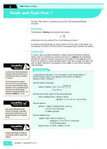
Research shows the following relationship between CD and Re for a sphere.

Fig. 2.8

For Re1

For a pseudo-plastic,

τy = 0 and n 1 then M2 1, i.e. the flow must be supercritical. The jump might occur because the slope of the bed is insufficient for friction to balance the loss of potential energy. Since the losses are smaller for the tranquil flow, the balance can be restored. A jump can be made to occur if there is an obstacle on the bed higher than the critical depth.

Figure 2

When the change occurs there is a reduction in momentum and an increase in the hydrostatic force. The solution is based on equating them. uo = mean velocity.

The mean depth is h/2

Pressure force on a cross section is Fp = ρgAh/2

Momentum force at a section =Fm = ρAu2

The cross sectional area is A = B h where B is the width. ρgA1h1 ρgA 2 h 2 ρgBh12 ρgB2 h 22 Change in pressure force = − = − 2 2 2 2 ρgB 2 ρgB (h1 − h 2 )(h1 + h 2 ) Change in pressure force = h1 − h 22 = 2 2

(

)

Change in momentum force = ρBh1u12 - ρBh2u22 = ρB(h1u12- h2u22) For continuity of flow u22 = ( u1 h1/ h2)2

⎛ h h 2 h12 2 ⎞ 2 ⎜ u 1 ⎟⎟ = ρBu 12 1 (h 2 − h1 ) Change in momentum force = ρB ⎜ h 1u 1 − 2 h2 h2 ⎝ ⎠ The change in pressure and momentum forces may be equated. ρgB (h1 − h 2 )(h1 + h 2 ) = ρBu12 h1 (h 2 − h1 ) 2 h2 g (h1 + h 2 ) = u12 h1 2 h2 ⎛h ⎞g u12 = (h1 + h 2 )⎜⎜ 2 ⎟⎟ ................(1) ⎝ h1 ⎠ 2 In terms of the flow rate ⎛h ⎞g g Q 2 = B2 h12 (h1 + h 2 )⎜⎜ 2 ⎟⎟ = B2 h1h 2 (h1 + h 2 ) 2 ⎝ h1 ⎠ 2

The flow per unit width is usually given as q 2 = gh1h 2 © D.J.DUNN www.freestudy.co.uk

3

(h1 + h 2 ) ....................(2) 2

(

)

2h1u12 2u 2 = h1h 2 + h 22 h 22 + h1h 2 − h1 1 = 0 g g h2 may be solved with the quadratic equation giving: From (1)

⎧ 8u 2 ⎫ ⎧ 8u 2 ⎫ 2h 2 = −h1 ± h1 ⎨1 + 1 ⎬ and since h2 cannot be negative 2h 2 = − h1 + h1 ⎨1 + 1 ⎬ ⎩ gh1 ⎭ ⎩ gh1 ⎭ u2 Substitute the Froude Number Fr2 = 1 2h 2 = − h1 + h1 1 + 8Fr2 gh1 h h 2 = 1 1 + 8Fr2 − 1 2

{

[{

}

}

]

Next consider the energy balance before and after the jump. Energy Head before the jump = h1 + u12/2g Energy Head after the jump = h2 + u22/2g Head loss = hL = h1 + u12/2g - h2 - u22/2g

hL = h1 - h2 + (u12 - u22)/2g h u 2 = u1 1 h2

Continuity of flow Q = u1 B h1 = u2 B h2 Hence

u12

− u 22

=

u12

2 ⎧ ⎛ h ⎞ 2 ⎫⎪ h1 ⎞ 2⎪ ⎟⎟ = u1 ⎨1 − ⎜⎜ 1 ⎟⎟ ⎬ h ⎝ 2⎠ ⎪⎩ ⎝ h 2 ⎠ ⎪⎭

⎛ - u12 ⎜⎜

⎛h ⎞g We already found equation (1) was u12 = (h1 + h 2 )⎜⎜ 2 ⎟⎟ ⎝ h1 ⎠ 2 Substitute 2 ⎛ h 2 ⎞ g ⎧⎪ ⎛ h1 ⎞ ⎫⎪ 2 2 u1 − u 2 = (h1 + h 2 )⎜⎜ ⎟⎟ ⎨1 − ⎜⎜ ⎟⎟ ⎬ ⎝ h1 ⎠ 2 ⎪⎩ ⎝ h 2 ⎠ ⎪⎭ u12 − u 22 =

2⎫ ⎛ ⎞⎧ 2 g (h1 + h 2 )⎜⎜ h 2 ⎟⎟⎨ h 2 −2 h1 ⎬ 2 ⎝ h1 ⎠ ⎩ h 2 ⎭

) g {(h

(

)}

+ h 2 ) h 22 − h12 2h1h 2 Substitute into the formula for hL

(u

2 1

− u 22 =

1

hL = h1 - h2 + (u12 - u22)/2g ( g(h1 + h 2 ) h 22 − h12 h1 + h 2 ) h 22 − h12 = (h1 − h 2 ) + h L = (h1 − h 2 ) + 2 x 2gh1h 2 4h1h 2

(

{

)

(

(

)}

hL =

4h1h 2 (h1 − h 2 ) + (h1 + h 2 ) h 22 − h12 4h1h 2

hL =

4h12 h 2 − 4h1h 22 + h 32 − h13 + h1h 22 − h12 h 2 4h1h 2

hL =

3h12 h 2 − 3h1h 22 + h 32 − h13 4h1h 2

hL

)

( h 2 - h1 )3 = 4h1h 2

Useful website © D.J.DUNN www.freestudy.co.uk

http://www.lmnoeng.com/Channels/HydraulicJump.htm 4

WORKED EXAMPLE No.1

50 m3/s of water flows in a rectangular channel 8 m wide with a depth of 0.5 m. Show that a hydraulic jump is likely to occur. Calculate the depth after the jump and the energy loss per second. SOLUTION

A1 = 8 x 0.5 = 4 m2 u1 = Q/A1 = 50/4 = 12.5 m/s Froude Number Fr1 = u/√gh = = 12.5/√(9.81 x 0.5) = 31.855 This is supercritical so a jump is possible. h 0.5 h 2 = 1 1 + 8Fr2 − 1 = 1 + 8 x 31.8552 = 3.748 m 2 2 A2 = 8 x 3.748 = 30 m2 u2 = Q/A2 = 50/30 = 1.667 m/s (h - h )3 (3.748 - 0.5)3 = 4.573 m hL = 2 1 = 4h1h 2 4 x 0.5 x 3.748 Energy loss = mghL = 50 000 x 9.81 x 4.573 = 2.243 MJ/s m = 50 000 kg/s

[{

}

]

SELF ASSESSMENT EXERCISE No. 1

1. Show by applying Newton's Laws that when a hydraulic jump occurs in a rectangular channel the depth after the jump is h h 2 = 1 1 + 8Fr2 − 1 2 ( h 2 - h1 )3 hL = Go on to show that the head loss is 4h1h 2 3 2. 40 m /s of water flows in a rectangular channel 10 m wide with a depth of 1.0 m. Show that a hydraulic jump is likely to occur. Calculate the depth after the jump and the energy loss per second. (Answers 1.374 m and 3.735 kJ/s)

[{

}

]

3. Water has a depth H = 1.5 m behind a sluice gate and emerges from the gate with a depth of 0.4 m. Downstream a hydraulic jump occurs. Calculate depth after the jump and the mean velocity before and after the jump. (Note use Bernoulli to find u1)

Figure 3 (Answers 1.416 and 1.627 m/s) © D.J.DUNN www.freestudy.co.uk

5

RISE IN LEVEL OF BED

In this section we will examine what happens to the level of water flowing in a channel when there is a sudden ride in the level of the bed.

Figure 4 First apply Bernoulli between points (1) and (2) u2 u2 h1 + 1 = h 2 + 2 + z 2g 2g uh From the continuity equation substitute u 2 = 1 1 h2 2

⎛ u1h1 ⎞ ⎜⎜ ⎟ 2 h 2 ⎟⎠ u1 ⎝ h1 + +z = h2 + 2g 2g

Rearrange

h1 +

u12 u 2h 2 − h 2 − 1 12 − z = 0 2g 2gh 2

⎞ ⎛ u2 u 2h 2 ⎜ h1 + 1 − h 2 − z ⎟h 22 − 1 1 = 0 ⎟ ⎜ 2g 2g ⎠ ⎝ Substitute h2 = x + h1 – z

{

}

⎧ ⎫ u12 (x + h1 - z )2 u12 2 ( ) ( ) + − + − + − =0 x h z z x h z h ⎨ 1 ⎬ 1 1 2g 2g ⎩ ⎭ 2 2 ⎧ u1 ⎫ u1 (x + h1 - z )2 2 =0 ⎨ − x ⎬(x + h1 - z ) − 2g ⎩ 2g ⎭

{

{u {u

2 1 2 1

} − 2gx }(x + h

}

− 2gx (x + h1 - z )2 − u12 (x + h1 - z )2 = 0 1-z

)2 − u12 (x + h1 - z )2 = 0

There follows a long bout of more algebra to produce a cubic equation for x : ⎛ ⎛ u2 ⎞ u2 ⎞ u2 x 3 + 2x 2 ⎜⎜ h1 − z − 1 ⎟⎟ + x (h1 − z )⎜⎜ h1 − z − 1 ⎟⎟ + z 1 (2h1 − z ) = 0 4g ⎠ g ⎠ 2g ⎝ ⎝ This equation may be used to solve the change in height of the water. If the values of x and z are small, we may neglect products and higher powers of small numbers so the equation simplifies to: ⎛ u 2 ⎞ zu 2 x ⎜⎜ h1 − 1 ⎟⎟ + 1 = 0 g ⎠ g ⎝ ⎛ u 2 ⎞ zu 2 x ⎜⎜1 − 1 ⎟⎟ + 1 = 0 ⎝ gh1 ⎠ gh1

© D.J.DUNN www.freestudy.co.uk

6

u1 hence gh1

The Froude number approaching the change is Fr1 =

(

2

)

2

x 1 − Fr1 + zFr1 = 0

x=

(F

zFr12

2 r1

− h1

)

The equation indicates that if flow is supercritical (Fr1>1) then x is positive and the surface rises. If the flow is sub critical (tranquil Fr1