Aug 25, 2013 - Ilmenau, Germany ... A cell is controlled by a base station (BS). ..... Base station time (and frequency) synchronization of base stations is ...
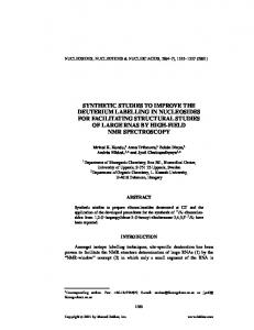
Coordinated Multi-Point in Cellular Networks From Theoretical Gains to Realistic Solutions and Their Potentials Tommy Svensson (Chalmers University) Mikael Sternad (Uppsala University) Wolfgang Zirwas (Nokia Solutions and Networks, Munich) Michael Grieger (TU Dresden) Tutorial at ISWCS‘2013 Ilmenau, Germany
INTRODUCTION
8/25/2013
Coordinated Multi-Point in Cellular Networks
Slide 2
Coordinated Multi-Point in Cellular Networks From Theoretical Gains to Realistic Solutions and Their Potentials
Michael Grieger TU Dresden
Mikael Sternad
Tommy Svensson
Uppsala University Chalmers Univ. of Technology (presenter) (presenter)
Wolfgang Zirwas Nokia Solutions and Networks (presenter)
This tutorial is based on cooperative work done in the EU research project
8/25/2013
Coordinated Multi-Point in Cellular Networks: Introduction
Slide 3
Coordinated Multi-Point in Cellular Networks From Theoretical Gains to Realistic Solutions and Their Potentials
Our story in a nutshell:
8/25/2013
Interference can be suppressed by coordinating multiple sites. This should theoretically provide large gains. But gains seem hard to attain in realistic settings. Message: Large gains can be attained, but you have to construct the solution carefully.
Coordinated Multi-Point in Cellular Networks: Introduction
Slide 4
Coordinated Multi-Point in Cellular Networks From Theoretical Gains to Realistic Solutions and Their Potentials
Our story in a nutshell:
Interference can be suppressed by coordinating multiple sites. This should theoretically provide large gains. But gains seem hard to attain in realistic settings. Message: Large gains can be attained, but you have to construct the solution carefully.
Outline:
8/25/2013
Theory and Practice: MIMO, Network MIMO and LTE status Key challenges and enablers for downlink joint transmission A harmonized downlink framework: Outcomes of the EU Artist4G Project Uplink aspects and Joint Detection
Coordinated Multi-Point in Cellular Networks: Introduction
Slide 5
Interference in Cellular Networks
Cellular networks:
Cell: Logical entity (with Cell-ID) within which transmission resources can be tightly controlled. A cell is controlled by a base station (BS). (3GPP eNB may control several cells/sectors.) Interference within cells controlled by resource allocation allocation (time, frequency, codes, spatial). BS2 Interference between cells remains.
BS3
UE3 UE1
SINR = useful received power interference + noise
UE2 BS1
Interference-limited cellular networks:
8/25/2013
Inter-cell interference (rather than noise) limits spectral efficiency. Example: LTE macro cellular systems with high load, outdoor users, inter-site distance (ISD) 500 m. Coordinated Multi-Point in Cellular Networks: Introduction
Slide 6
Frequency Reuse Factor > 1 The traditional way of controlling inter-cell interference
Frequency (transmission resource) reuse factor n:
Area is covered by regular clusters of n cells. Each cell in a cluster uses different orthogonal transmission resources. Distance to nearest interferers in neighbouring clusters (”reuse distance”) increases with n. => Inter-cell interference will decrease with n.
But: The fraction of total resources available in each cell is then 1/n n=3:
(Heterogenous networks complicate the picture) 8/25/2013
Coordinated Multi-Point in Cellular Networks: Introduction
Slide 7
Coordinated MultiPoint Transmission (CoMP) Sharing of User Data? Two basic options:
Coordinate transmission/reception within a Cooperation Area (CA) => More flexible interference control than static frequency reuse. CoMP without sharing of user data: Data to/from single user via one point: Coordinated scheduling Coordinated beamforming Inter-Cell Interference Coordination (ICIC, eICIC, feICIC).
(ICIC, eICIC,
CoMP with sharing/distribution of user data (higher potential gains): A main focus of this tutorial Joint Transmission (JT) in downlinks (coherent or non-coherent). Joint Detection (JD) in uplinks. 8/25/2013
Coordinated Multi-Point in Cellular Networks: Introduction
Slide 8
CoMP Architectures Coordinate transmission/reception within a Cooperation Area (CA) => More flexible interference control than static frequency reuse.
[Source: Winner+ Project]
Possible coordinated entities: Remote Radio Units (RRUs) Cells with intra-site or inter-site coordination Relay nodes (RNs). May use multi-cell coordination with BSs, RRUs and RNs within the cells. 8/25/2013
Coordinated Multi-Point in Cellular Networks: Introduction
Slide 9
Some History:
1983: F. M. J.Willems and M.J. Frans: “The discrete memoryless multiple access channel with partially cooperating encoders” 2000: T. Weber, Meurer, P.W. Baier: JT/JD for TD-CDMA Chinese-Siemens Cooperation Project ‚FUTURE‘ CoMP activities in China
Joint transmission (JT) or joint reception (JR) for local area ‚Service Area‘ Concept 2001-2004: Theoretical investigations, e.g. [Shamai et.al. 2001,2002], [Jafar et. al. 2002,2004]. 2003: COVERAGE project: ‚cooperative multi stage relaying‘ 2004: 3GET project extension of Service Area Concept to macro-cellular networks 2005-2006: Series of theoretical investigations finding large potential gains (Foschini et.al.) 2010: German project ‚Easy C‘: CoMP testbeds in Dresden and Berlin 2010-2012: EU FP7 ARTIST4G project (Used the CoMP testbeds in Dresden) 3GPP LTE Rel 10: CoMP Study Item / Rel 11 CoMP Work Item 3GPP LTE Rel 11: No supporting functions for JT CoMP, due to challenging time-/frequency synchronization. Coordinated Multi-Point in Cellular Networks: Introduction
Slide 10
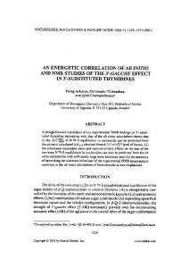
Motivations for CoMP 1. Overcome interference limitations in cellular radio networks Reduce gap between single- and multi-cell performance.
Large theoretical network capacity gains for network-wide and coherent joint transmission: minimal SNIR [dB]
cooperative BS
γ
conventional cellular [Source: Distributed Antenna
total Tx power [dBm]
Systems by M. Schubert et.al.]
Mechanisms for interference control:
Interference avoidance, by Coordinated scheduling/beamforming. Most effective at low-to-medium loads (taking fairness into account).* Interference cancellation: Coherent joint transmission reduces interference by cancellation. Works also at high loads (if channel estimates are good).
*[See e.g. 3GPP TR 36.819 V11.0.0] 8/25/2013
Coordinated Multi-Point in Cellular Networks: Introduction
Slide 11
Motivations for CoMP 2. Coverage gains
A more even distribution of capacity and user experience between cell center and cell edge UEs:
[Source: Artist4G project]
Flexibility: Allocate capacity to where the users are active.
Reduce power/noise limitations for highly shadowed UEs.
Exploit macro diversity gains, including MIMO channel rank improvements.
8/25/2013
Coordinated Multi-Point in Cellular Networks: Introduction
Slide 12
Motivations for CoMP 3. Efficient use of existing infrastructure
Cooperative transmission over several cells and sites using already deployed antennas and RF front-ends.
Enable multi-user MIMO transmission/reception (network MIMO) with cooperating (distributed) antennas at the network side.
But… This requires adequate communication/coordination links and intelligence within the cooperation areas. Antennas/BSs will have different distances to a user. Can they then still cooperate efficiently? If not always, then under what conditions? (Cancelling weak interference components can provide significant SINR gains.) 8/25/2013
Coordinated Multi-Point in Cellular Networks: Introduction
Slide 13
Cooperation Areas
Different degrees of cooperation have different influence on interference
No Cooperation
Full Cooperation
Strong interference between cells Interference completely avoided Needs full CSI for the whole network (not realistic)
Strong Interference without cooperation
Interference completely avoided by full cooperation
Cooperation area ('CA')
Cooperation only inside of a limited number of sectors Interference just between cooperation areas Coordinated Multi-Point in Cellular Networks: Introduction
Slide 14
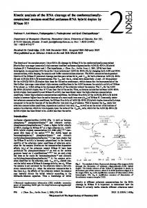
However…. Theoretical versus simulated CoMP gains:
minimal SNIR [dB]
cooperative BS
3GPP
3GPP γ
conventional cellular total Tx power [dBm]
[Source: Foschini et.al. 2006]
MU-MIMO 2x2
Where do we loose??
MU-MIMO 4x2 MU-MIMO 8x2
Are there fundamental limits?? [Source: 3GPP,
JT MU-MIMO 2x2
JT MU-MIMO 4x2
TR 36.819 V11.0.0 (2011-09), Table 7.2.1.2-5]
source 1 source 3 source 12
ULA
JT MU-MIMO 8x2
Cell avg Cell-edge Cell avg Cell-edge Cell avg Cell-edge 9 cells Cell avg Cell-edge > 9 cells Cell avg Cell-edge 9 cells Cell avg Cell-edge > 9 cells Cell avg Cell-edge 9 cells Cell avg Cell-edge
2.069 0.0548 3.163 0.0863
1.86 0.058
[Source: M. Schubert et.al.]
reference Rel10
3.05 0.1 4.5 0.151 2.77 0.107
2.713 0.0879 2.35 0.102
27% gain
best JT result in
4.028 0.1368
3GPP CoMP SI
2.81 0.139
(ideal) 6.11 0.207
Slide 15
How to attain more of the theoretical gains?
A preview of where we are heading: 1. Cooperation areas have to be designed carefully to provide gains for most users. 2. Interference from outside the CA needs to be reduced so that it does not swamp the intra-CA gains. 3. Groups of users that cooperate in a resource block need to be selected well, but still fast and efficiently.
8/25/2013
Coordinated Multi-Point in Cellular Networks: Introduction
Slide 16
How to attain more of the theoretical gains?
A preview of where we are heading: 1. Cooperation areas have to be designed carefully to provide gains for most users. 2. Interference from outside the CA needs to be reduced so that it does not swamp the intra-CA gains. 3. Groups of users that cooperate in a resource block need to be selected well, but still fast and efficiently. Additional important aspects and practical constraints: Channel estimation/prediction accuracy Channel reporting feedback: accuracy and load in FDD Transmit power constraints Control signalling load, data distribution load limits Time synchronization limitations to/from multiple sites. (All these issues e.g. limit the practical cooperation area size.) 8/25/2013
Coordinated Multi-Point in Cellular Networks: Introduction
Slide 17
Coordinated Multi-Point in Cellular Networks From Theoretical Gains to Realistic Solutions and Their Potentials
Main aspects/techniques in focus in this Tutorial:
System design aspects, inter-relationships that affect the performance Joint transmission/detection (for performance reasons) Centralized coordination (for performance reasons) Linear, mainly coherent, precoding (complexity and performance).
Outline: Theory and Practice: MIMO, Network MIMO and LTE status Key challenges and enablers for downlink joint transmission A harmonized downlink framework: Outcomes of the EU Artist4G Project Uplink aspects and Joint Detection
8/25/2013
Coordinated Multi-Point in Cellular Networks: Introduction
Slide 18
THEORY AND PRACTICE
8/25/2013
Coordinated Multi-Point in Cellular Networks
Slide 19
Section Overview
Precoding and equalization
Multi-user MIMO systems
Network MIMO systems
Toy scenario results
Practical impairments
3GPP results
8/25/2013
Coordinated Multi-Point in Cellular Networks: Theory and Practice
Slide 20
From MIMO to Network MIMO MIMO Precoding and Equalization
singular value decomposition (SVD) and parallel channels
A matrix can be decomposed such that
TX
RX
Linear spatial precoding and equalization parallelizes the channel into its Eigenmodes This opens the door for power control (waterfilling) to maximize capacity use all modes in case of high SNR one or few strongest modes in case of low SNR optimal because Shannon formula is concave in the power Precoding requires transmitter CSI
8/25/2013
Coordinated Multi-Point in Cellular Networks: Theory and Practice
Slide 23
From MIMO to Network MIMO Multi-User MIMO
MIMO multiple access system, Uplink: Equalization
UE1 UE UE2
BS demapping demodulation decoding
UEK K 8/25/2013
UEs might transmit one or several data streams Spatial equalization (decorrelation) done at the BS Links of UEs experience different pathloss & large scale fading that might be compensated by power control Timing of received signals at BS can be aligned using timing advance Coordinated Multi-Point in Cellular Networks: Theory and Practice
1
2
Slide 25
From MIMO to Network MIMO Multi-User MIMO
Multi-user MIMO (broadcast channel), Downlink:
UE1 coding modulation mapping
Precoding
BS
UE2
UEK CSI at transmitter required to separate Tx streams at receivers Dirty paper coding is capacity achieving Linear precoding techniques (e.g. ZF for channel inversion at the transmitter) allow min(Nbs,NUE) increase of data rate at high SNR Potentially, combination of precoding and equalization if UEs are equipped with several receive antennas
8/25/2013
Coordinated Multi-Point in Cellular Networks: Theory and Practice
Slide 26
From MIMO to Network MIMO network MIMO
Consider a cellular system with frequency reuse one High performance when users located in vicinity of assigned base stations Interference problem when users are located at cell edges In general: Cellular communications systems with independent base stations are interference limited -> low SINR at cell edges
network MIMO to
Jointly transmit/detect Mitigate interference Increase spectral efficiency
However
Base station time (and frequency) synchronization of base stations is required Received symbol timing cannot be aligned due to propagation delays on different paths Coordinated Multi-Point in Cellular Networks: Theory and Practice
Slide 27
From MIMO to Network MIMO network MIMO
cell edge 1
2
pathloss exponent = 3.5 omnidirectional antennas dsite = 2000 m cell-edge SNR = 18 dB Nue = 2, Nbs = 2 Uncorrelated Rayleigh fading no shadow fading ML receiver
Potentially larger gains in cellular systems due to shadowing due to universal frequency reuse
8/25/2013
Coordinated Multi-Point in Cellular Networks: Theory and Practice
Slide 28
From MIMO to Network MIMO network MIMO
[Source: Foschini et.al. 2006]
pathloss exponent = 3.8 coordination in user centric clusters of 19 cells no outer cluster interference dsite = 500 m cell-edge SNR = 18 dB (strong interference limitation) Uncorrelated Rayleigh fading shadow fading included perfect transmitter CSI
[Source: Foschini et.al. 2006] 8/25/2013
Coordinated Multi-Point in Cellular Networks: Theory and Practice
Slide 29
Current Status in 3GPP CoMP Scenarios used for evaluation
Homogeneous as well as heterogeneous scenarios with macro cells and low power nodes
1) intra site CoMP
2) homogeneous inter site CoMP
3) heterogeneous setup independ cell ID
4) heterogeneous setup same cell ID
[Source: Lee et.al. 2012] 8/25/2013
Coordinated Multi-Point in Cellular Networks: Theory and Practice
Slide 35
Current Status in 3GPP 3GPP simulated CoMP gains
source 1 source 3 source 12
ULA MU-MIMO 2x2 MU-MIMO 4x2 MU-MIMO 8x2 JT MU-MIMO 2x2
[Source: 3GPP,
JT MU-MIMO 4x2
TR 36.819 V11.0.0 (2011-09), Table 7.2.1.2-5]
JT MU-MIMO 8x2
Cell avg Cell-edge Cell avg Cell-edge Cell avg Cell-edge 9 cells Cell avg Cell-edge > 9 cells Cell avg Cell-edge 9 cells Cell avg Cell-edge > 9 cells Cell avg Cell-edge 9 cells Cell avg Cell-edge
2.069 0.0548 3.163 0.0863
1.86 0.058
reference Rel10
3.05 0.1 4.5 0.151 2.77 0.107
2.713 0.0879 2.35 0.102
27% gain best JT result in
4.028 0.1368
3GPP CoMP SI
2.81 0.139
(ideal) 6.11 0.207
Current Status in 3GPP Up to 8 transmit antennas in the downlink Differences between theory and 3GPP:
Rayleigh channel models in theory, SCM in 3GPP Evaluations with perfect channel estimation also in 3GPP Network wide (theory) vs. clustered (3GPP) precoding Outdoor to indoor penetration loss in 3GPP leads to noise limitation.
Tools for interference measurements in Release 11 No specific support for joint transmission CoMP in Release 11
Improved feedback would need to be standardized No new Reference symbols
Specification for MIMO can potentially be used for CoMP as well
CSI reference symbols defined in Release 10 probably adequate Channel feedback
Uplink joint detection can potentially be implemented without changes on the air interface. 8/25/2013
Coordinated Multi-Point in Cellular Networks: Theory and Practice
Slide 37
Theory and Practice Main messages of Section
What we learned from theory Linear MIMO gain requires high S(I)NR and uncorrelated channel realizations. Cell edge SINR in a non-cooperative cellular system is very low due to inter-cell interference or penetration loss for indoor users. Joint signal processing (network MIMO) can be used to exploit inter-cell propagation. Large gains of joint signal processing in toy scenarios and simplified system level simulations with network wide cooperation. What we see in practical implementations Additional practical impairments. 3GPP system level simulation results show small network MIMO gains. 8/25/2013
Coordinated Multi-Point in Cellular Networks: Theory and Practice
Slide 38
EVALUATION OF KEY CHALLENGES AND ENABLERS FOR DOWNLINK JOINT TRANSMISSION 8/25/2013
Coordinated Multi-Point in Cellular Networks
Slide 39
Downlink JT Key Challenges and Enablers Signal Processing and System Design
Transmitter CSI
Channel estimation, accuracy requirements CSI feedback: Outdating, overhead and quantization Channel prediction Zero-forcing linear precoding Use of accuracy estimates in robust linear precoders
Complexity of network wide cooperation
Clustering: Cooperation areas Inter-cluster interference floor, complexity of cooperation
Backhaul aspects (topologies, technologies, capacity, latency) Time and frequency synchronization of base stations
8/25/2013
Coordinated Multi-Point in Cellular Networks: Challenges and Enablers
Slide 40
CSI: Special Needs for Downlink CoMP Channel estimation and prediction
Coordinated beamforming requires information on ”forbidden” directions /signal subspaces for interference avoidance.
Coherent joint transmission furthermore requires accurate channel phase estimates for interference cancellation. Signal subtraction (interference cancellation) is sensitive:
Channel estimates from several base stations in cooperation area:
Adequate estimation quality for the weakest channels? Orthogonal reference signals within CA: density/overhead tradeoff.
FDD Downlinks: Uplink reporting load for channel estimates.
Non-static users, transmission feedback delay + CoMP delays => Channel outdating. Problems already at pedestrian velocity. => Need for channel prediction, based on most recent estimates.
Residual phase rotation of channels (synchronization inacuracies, phase noise) can be tracked by channel predictors.
8/25/2013
Coordinated Multi-Point in Cellular Networks: Challenges and Enablers
Slide 41
CSI: Channel Estimation, LTE Rel 10 CSI RSs - including interference floor shaping. Ref. signal SIR statistics
8
1..4
LTE Rel.10 CSI 5..8 RS: 40RE 7
9
2 29..32
8
1..4 7
3
2 29..32
9..1 2
3
33..36
25..28 8
1..4
20..24
3
5 13..16
33..36
25..28
7
33..36
9..1 2
20..24
2 29..32
33..36 5 13..16
8
20..24
1..4 7
9..1 2
33..36
25..28
2 29..32
3
5 13..16
33..36
1..4
17..20 4
25..28 8
1..4
20..24 7
9..1 2
25..28
7
5..8
9
6 2 29..32
3
5 13..16
9..1 2
5 13..16
17..20 4
1
5..8
33..36 17..20 4
1
5..8
8
5 13..16
9
6
25..28
6
0
-20
6
20..24
20
40
60
SIR [dB]
20..24
subset of orthogonal CSI RSs
6
20..24
17..20 4
1
3
9..1 2
17..20 4
25..28
5..8
1
5..8
9
6
2 29..32
3
17..20 4
1
3
20..24
1..4
1
5..8
9
9..1 2
2 29..32
7
9
6
9
6
7
2 29..32
81..4
17..20 4
1
1..4
17..20 4
25..28
33..36 5 13..16
8
5 13..16
1
5..8
9
9..1 2
muting patterns: simultaneously active sites have same colour
large minimum distance between simultaneously active CSI RSs
Coordinated Multi-Point in Cellular Networks: Challenges and Enablers
Slide 42
CSI Feedback Outdating, overhead and quantization for Centralized joint transmission
FDD systems:
Outdating: Feedback +proc.delay(5 ms) +2 x Backhaul latency(1-20ms). Problematic at pedestrian velocities at > 2.0 GHz carriers. Uplink overhead: A few Mbit/s over a 10-20 MHz uplink* (complex numbers or gain + phase).
TDD systems: Using uplink estimates for downlink: Outdating: 2 x Backhaul latency. Overhead: Uplink pilots from all users, in all utilized RBs, detected in all cells. Out-of CA-interference is not reciprocal. May need uplink feedback as in FDD.
Quantization: 8 bits per complex channel results in small linear precoder performance loss. Should also report CSI reliability! *[EU FP7 Artist4G Project Deliverable D1.4, Section 5.3.3. https://ict-artist4g.eu/ ] 8/25/2013
Coordinated Multi-Point in Cellular Networks: Introduction
Slide 43
CSI: Channel Prediction Performance using Kalman prediction (optimal linear MMSE prediction) Example: Predicting 4 channels for •
Different Doppler spectra
•
Ref. signal SIR = 6 ,12 & 18 dB. 6 dB
e.g. prediction NMSE -10 dB (indicated) is attainable for 0.1- 0.3 wavelength horizon, or 8 ms – 24 ms at 5 km/h at 2.66 GHz. Attainable dB cancellation by coherent JT CoMP = Normalized Mean Square Error (NMSE) of channel estimates.
12 dB
Flat Doppler spectrum: (Hard to predict)
18 dB Frequency selective Flat fading
Jakes (Rayleigh fading) Doppler spectrum:
Residual phase rotation due to synch. error with jitter
[See Daniel Aronsson, Channel Estimation and Prediction for MIMO OFDM Systems: Key design aspects of Kalman-based algorithms. PhD Thesis, Signals and Systems, Uppsala University, March 2011, Chapter 6.5.] 8/25/2013
Coordinated Multi-Point in Cellular Networks: Challenges and Enablers
Slide 44
CSI: Zero-Forcing (ZF) Linear Precoder using estimated/predicted channels from transmitters in CA Downlink channels within OFDM resource block: Complex matrix H. Pre-inversion by zero forcing precoder W when estimate Hˆ is invertible:
1 W Hˆ D
When # transmitters > # receiver antennas within cooperation area: Regularized pre-inversion or Moore-Penrose pseudoinverse: 1 1 W Hˆ * Hˆ Hˆ * D W Hˆ * Hˆ Hˆ * D
The precompensated channel matrix is ideally HW D
The „target matrix“ D is (block)diagonal and contains per-stream gains. These gains can be optimized to maximize e.g. a weighted sum rate, under per transmit antenna power constraints. Large eigenvalue spread of channel matrix leads to precoders that have small gains for nearest BS => Still interference cancellation, but bad SNR. Power normalization loss problem. 8/25/2013
Coordinated Multi-Point in Cellular Networks: Challenges and Enablers
Slide 45
CSI: Robust Linear Precoder Taking channel accuracy (covariance) information into account
Kalman predictors provide prediction uncertainty Ē{ΔH*ΔH}. CoMP precoder should be designed by taking all relevant information into account.
J E E V (t ) E Su(t ) 2
2
We may use a scalar criterion:
* * * * * The precoder minimizing J is then:* R Hˆ V VHˆ S S E H V VH
1
Hˆ *V *VD
Weights V and S can be adjusted iteratively to optimize SINR, local capacity, utility…**
Robust Linear Precoder
(block)diagonal Target matrix * K. Öhrn, A. Ahlén and M. Sternad, ”A Probabilistic approach to multivariable robust filtering and open-loop control”, IEEE Trans. on Autom. Contr, vol. 40, March 1995, pp. 405-417 . ** R. Apelfröjd, M. Sternad and D. Aronsson ”Measurement-based evaluation of robust linear precoding in downlink CoMP”, IEEE ICC 2012, Ottawa . 8/25/2013
d(t)
Transmit symbols for M users
u(t)
Transmit signal, N transmitters.
y(t)
Received signal excl. noise
z(t)
Target signals at receivers
ε(t)
Error signal
R
Precoding matrix (N x M)
H
Channel matrix
Hpred
Predicted channel matrix
ΔH
Prediction error matrix, E(ΔH)=0
D
Target system (M x M), diagonal
S
Transmit power penalty matrix (N x N), usually diagonal, ≥ 0
V
Error penalty matrix (M x M),>0
c
Scalar transmit scaling factor
Coordinated Multi-Point in Cellular Networks: Challenges and Enablers
(M-vector) (M x N)
Slide 46
CSI: Accuracy Requirements per CA - example ARTIST4G
8
ˆ H H H W pinv (H) ˆ pinv (H ˆ) W ˆ W W - W ˆ; Yˆ HW Heterogenous Backhaul networks => Inter-BS connections with heterogeneous connectivity, capacity and latency. 8/25/2013
Coordinated Multi-Point in Cellular Networks: Challenges and Enablers
Slide 53
Synchronization Issues Time- and frequency synchronization btw eNBs:
is essential basic enabler In 3GPP sometimes argument against JT CoMP
eNB1 OFDM symbol
eNB 2
GI should cover: tsync + delay spread + 1-2
Requirements [ LTE: SC spacing 15kHz, SF length 1ms, GI: 4.7s, FB delay 10ms ]: within fraction of an OFDM guard interval (< one to very few s)
Time:
Frequency: ideally below 0.1ppb at RF of 2.6GHz Phase Noise (>100Hz): can’t be compensated requires high Q LOs
Options for frequency synchronization:
GPS + tight synchronization with extremely stable TXOs (see demo systems) IEEE 1588v2 - precision time protocol (PTP): avoids GPS, accuracy unclear over the air synchronization: based on UE feedback (single value per eNB!) CSI reporting with channel prediction e.g. based on simple linear prediction Coordinated Multi-Point in Cellular Networks: Challenges and Enablers
Slide 54
Frequency Synchronization A) Inter carrier interference: neglectable for typical f of about 100Hz
B) inter eNB phase drift: = 10ms and f= 100Hz (10ms) = 0.01*100Hz= 360° !!! tight synchronization or (linear) CSI prediction ! 0.1 ppb (7ms) = 0.007*0.26Hz= 0.6° !!!
(, f)
A) Inter carrier interference 1
0.8
SIR >20dB
0.6
0.4
0.5 ppb 2 ppb = 70s 5 ppb 0.007 ppb 0.03 ppb = 7ms 0.1 ppb
0.2
0
-0.2
-0.4
0
50
100
150
200
250
300
350
400
450
Inter carrier interference for f=500Hz LTE: f= predefined threshold.
Y = H * W’,
W’ is precoder matrix calculated for partially reported CSI
channel matrix H: 27UE x 36WB beams
UE #
13 CC >-6dB 47 CC > -12dB 46 CC > -18dB 47 CC > -24dB 185 CC > -30dB unreported WB beam #
off diagonal elements due to precoding errors require careful system design Coordinated Multi-Point in Cellular Networks: Artist4G Harmonized Framework
Slide 63
Interference Floor Shaping
8/25/2013
Coordinated Multi-Point in Cellular Networks: Artist4G Harmonized Framework
Slide 64
Rate Regions versus Interference Floor noise floor:
R1
low for IF limited scenarios max MCS R1max
rate region w IF floor
R2
rate region w/o CoMP optimum rate region for CoMP
max MCS R2max
Significant loss due to IF floor & small gain over non CoMP case Coordinated Multi-Point in Cellular Networks: Artist4G Harmonized Framework
Slide 65
Interference Floor Shaping: ‘Tortoise’ Concept
Goal: Reduce inter-CA interference
7° tilt / 46dBm
Tortoise Concept: Generate tortoise like power distribution per CA by cell specific antenna tiltings: CA center/outbound wideband beams with low/strong tilt & strong/low Tx power
15° tilt
40dBm
Per cover shift, serve mainly CA-centric UEs (CA edge UEs are scheduled into other best fitting cover shift.)
Benefits: Approaching network wide cooperation gains Robust and simple solution (e.g. use active antennas) Decoupling of CAs optimization per CA possible. Coordinated Multi-Point in Cellular Networks: Artist4G Harmonized Framework
Tortoise like shape of
Rx power over location
Slide 66
Interference Floor Shaping: Evaluation by ray tracing simulation RX power for single tortoise (3 sites) in Schwabing area of Munich red: CA center with zero dB Rx power
fast decline of IF power green: Rx power Coherent JT CoMP problematic for random user locations
Coordinated Multi-Point in Cellular Networks: Artist4G Harmonized Framework
Slide 71
Two Stage Scheduling Strategy Stage 1: Scheduling (and MU-MIMO) designed per cell
Goal:
8
Suitable performance versus complexity trade off Reuse current LTE schedulers as far as possible
7 9 5
2
4
1
Approach: Exploit inherent physical channel properties
3
6
single CAs
Co-located antenna elements per cell with high correlation in depth optimization per cell: ‘Exhaustive’ search of optimum user groups per cell (3 out of 10 UE) Proportional fair scheduling btw user groups MU frequency scheduling gain Include feedforward DL signaling for advanced Rx receivers (IRC-MMSE)
low correlation between sites exploit rank enhancements
Tortoise Optimization per CA sufficient
Result from this cell-specific user selections and beamforming: User grouping. Sets of users in the CA with much better conditioned CA-wide channel matrices. 8/25/2013
Coordinated Multi-Point in Cellular Networks: Artist4G Harmonized Framework
Slide 72
Two Stage Scheduling Strategy Stage 2: CA-wide precoder design w. user groups by Stage 1 stage 2) calculate CA wide precoder for per cell user groups + robust precoding + some fine tuning Cooperation area CAb
scheduler
site s2
site s1 Cell1
Cell 2
Cell 3
scheduler scheduler scheduler
site s3 Cell M scheduler
stage 1) exhaustive search of best user group including opt. precoder
NBS=4
NUE=2
K=10 UEs per celll
Note: Cell schedulers assume no inter cell interference single cell MU MIMO Coordinated Multi-Point in Cellular Networks: Artist4G Harmonized Framework
Slide 73
Relative Performance Gains (ideal CSI) Main evaluation case: 4 Tx, 2 Rx antennas, 3 site (9 cell) CAs
SINR [dB] cell edge
average
Spectral efficiency bits/s/Hz/cell
Network wide CoMP (1)
-
-
8 / 15(2)
160
Network wide CoMP with nonlinear precoding(1)
-
-
11 / 20
250
3GPP MU-MIMO
-
-
3.1
0 (reference)
3GPP JP-CoMP
-
-
4.0
30
9-cell CoMP (3)
-2
12
-
-
+ cover shift (3)
4
17
-
-
+ IF floor shaping (3)
12
23
-
-
+ 2-stage scheduler (4)
5
15
7.5 / 13 (2)
140
SE gain [%]
(1) Simulation conditions are not fully comparable; higher values are for nonlinear precoding (2) Values after backslash ignore LTE overhead of 43%; (3) SINR for single UE per cell and for 4x2; (4) SINR for 2 to 3 out of 10 simultaneously scheduled UEs per cell and 4x2 configuration Perfect transmitter CSI assumed in all evaluations above.
SINRs [dB] for single UE per cell
Coordinated Multi-Point in Cellular Networks: Artist4G Harmonized Framework
WP1
Slide 74
/25
Downlink JT CoMP Performance with Imperfect CSI
8/25/2013
Coordinated Multi-Point in Cellular Networks: Artist4G Harmonized Framework
Slide 75
Effects of Channel Estimation and SNR Main evaluation case: 4 Tx, 2 Rx antennas, 3 site (9 cell) CAs
Effects of SNR and Channel estimator interpolation gains (IPG) = – (SNR-NMSE) [dB]. spectral efficiency over UE noise figure in [dB) with IPG=3 / 12 / 30 / 50 dB 8
some fine tuning included
IPG
PL 20dB
6 [b/s/Hz/cell] SE SE [b/s/Hz/cell]
0 dB 12 dB 30 dB 50 dB
7
UE NF 9dB 5
similar 3GPP case 1
4
PL 0dB UE NF 7dB
3
maximize SNR !
2 1 -15
-10
0 -15
-5
-10
5
0
-5
10
0
enhance CSI prediction ! 20 15 25 5
10
NF in [dB]
NF [dB)
15
20
25
30
Penetration Loss (PL)+ 3dB default UE Noise Figure (NF) in [dB] PL: outdoor to indoor penetration loss; IPG: Interpolation Gain Coordinated Multi-Point in Cellular Networks: Artist4G Harmonized Framework
WP1
Slide 76
/25
Performance Example. 1: Channel prediction Using channel sounding data from Stockholm (by Ericsson) Simultaneous Kalman prediction of single-antenna channels from three sites:
latitude
Measurements: - Single-antenna transmitters 59.245 - 20 MHz OFDM channels 59.244 - 15 kHz subcarriers - 2.66 GHz carrier - Upsampled from 30 to 5 km/h 59.243 Channel prediction: - Orthogonal ref. signals, - Total RS overhead 1/9, - Frequency-domain Kalman based on AR4 fading models. Average (over positions and subcarriers) prediction NMSEs, at noise level -120 dBm:
17.568
17.57 longitude
17.572
Prediction horizon (wavelengths)
In ms, at 5km/h
NMSE, weakest of 3 channels (Kalman)
Average NMSE for all channels (Kalman)
[By using outdated CSI:]
0
0 ms
- 12.7 dB
- 23.9 dB
- 23.9 dB
0.06
5 ms
- 9.4 dB
- 15.3 dB
- 12.5 dB
0.13
10 ms
- 7.4 dB
- 12.9 dB
- 7.9 dB
0.19
15 ms
- 5.9 dB
- 11.2 dB
- 5.0 dB
0.28
23 ms
- 4.1 dB
- 9.2 dB
- 2.1 dB
[EU FP7 Artist4G Project Deliverable D1.4, Appendix A4-2. https://ict-artist4g.eu/ ] 8/25/2013
Coordinated Multi-Point in Cellular Networks: Artist4G Harmonized Framework
Slide 77
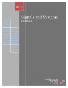
Performance Example. 2: User Grouping Two-stage scheduler for three single-antenna BS
The User groups are directly generated by the cellular scheduling Each user is allocated to a cell within the CA (the strongest BS). Scheduling performed per cell on orthogonal time-frequency resource blocks. A CA-wide joint transmission linear precoder is then designed for each RB. All users in a RB belong to different BS/cells. They have different strongest BS. Diagonal-dominant and well conditioned 3 x 3 channel matrices for each RB. “Cellular grouping”
RB
Example:
BS3
UE2
UE3
UE4
UE5
UE6
1 2
UE3
BS2
UE1
UE1 UE2