Hindawi Publishing Corporation Mathematical Problems in Engineering Volume 2013, Article ID 806325, 13 pages http://dx.doi.org/10.1155/2013/806325
Research Article Two-Agent Single-Machine Scheduling of Jobs with Time-Dependent Processing Times and Ready Times Jan-Yee Kung,1 Yuan-Po Chao,1 Kuei-I Lee,2 Chao-Chung Kang,3 and Win-Chin Lin4 1
Department of Business Administration, Cheng Shiu University, Kaohsiung 1037, Taiwan Department of Hospitality Management, Tunghai University, Taichung 1001, Taiwan 3 Department of Business Administration and Graduate Institute of Management, Providence University, Taichung 1008, Taiwan 4 Department of Statistics, Feng Chia University, Taichung 1007, Taiwan 2
Correspondence should be addressed to Yuan-Po Chao;
[email protected] Received 22 May 2013; Accepted 18 June 2013 Academic Editor: Yunqiang Yin Copyright © 2013 Jan-Yee Kung et al. This is an open access article distributed under the Creative Commons Attribution License, which permits unrestricted use, distribution, and reproduction in any medium, provided the original work is properly cited. Scheduling involving jobs with time-dependent processing times has recently attracted much research attention. However, multiagent scheduling with simultaneous considerations of jobs with time-dependent processing times and ready times is relatively unexplored. Inspired by this observation, we study a two-agent single-machine scheduling problem in which the jobs have both time-dependent processing times and ready times. We consider the model in which the actual processing time of a job of the first agent is a decreasing function of its scheduled position while the actual processing time of a job of the second agent is an increasing function of its scheduled position. In addition, each job has a different ready time. The objective is to minimize the total completion time of the jobs of the first agent with the restriction that no tardy job is allowed for the second agent. We propose a branch-andbound and several genetic algorithms to obtain optimal and near-optimal solutions for the problem, respectively. We also conduct extensive computational results to test the proposed algorithms and examine the impacts of different problem parameters on their performance.
1. Introduction In many scheduling models researchers assume that the job processing times are known and fixed parameters. However, the job processing times can be prolonged due to deterioration or shortened due to learning over time in real-life situations. Browne and Yechiali [1] present fire-fighting as an example of job deterioration while Biskup [2] cites workers’ skill improvement as an example of job learning. Both examples and their corresponding situations are referred to as “time-dependent scheduling” in the literature. Time-dependent scheduling was first introduced by J. N. D. Gupta and S. K. Gupta [3] and Browne and Yechiali [1] for deterioration jobs, whereas by Biskup [2] for the learning effect. Since then, a lot of scheduling models involving job time-dependent processing times have been proposed from a variety of perspectives. For more detailed reviews of scheduling problems with deteriorating jobs, we refer the reader to Alidaee and Womer [4] and Cheng et al. [5], and for a detailed review of scheduling problems with learning effects, we refer
the reader to Biskup [6]. More recently, scheduling research that considers both deteriorating jobs and learning effects has become popular. For details on this stream of scheduling research, the reader may refer to Wang [7], Wang and Cheng [8, 9], Wang and Liu [10], Wang and Guo [11], Zhang and Yan [12], Yang [13], and Zhu et al. [14], among others. In the past, the scheduling literature was dominated by studies that deal with a single criterion. In reality, jobs might come from several agents (customers) that have different requirements to meet. However, scheduling research in the multiple-agent setting involving jobs with time-dependent processing times is relatively unexplored. Among the few studies on this topic, Liu and Tang [15] studied multiagent scheduling with deteriorating jobs in which they assumed that the actual processing time of job 𝐽𝑗 is 𝛿𝑗 𝑡, where 𝛿𝑗 > 0 and 𝑡 denote the deteriorating rate and starting time of 𝐽𝑗 , respectively. Liu et al. [16] considered two two-agent problems with position-dependent processing times. In the aging-effect model, they assumed that the actual processing time of 𝐽𝑗 is 𝑝𝑗 + 𝑏𝑟 (𝑝𝑗 + 𝑏V) if it belongs to agent 𝐴(𝐵).
2
Mathematical Problems in Engineering
Meanwhile, in the learning-effect model, they assumed that the actual processing time of 𝐽𝑗 is 𝑝𝑗 − 𝑏𝑟 (𝑝𝑗 − 𝑏V) if it belongs to agent 𝐴(𝐵), where 𝑟 (or V) denotes the job position and 𝑏, 𝑏 > 0, is the aging or learning effect. Cheng et al. [17] considered a two-agent scheduling problem in which they assumed that, given a schedule, the actual processing time of a job of the first agent is a function of position-based learning while the actual processing time of a job of the second agent is a function of position-based deterioration. The objective is to minimize the total weighted completion time of the jobs of the first agent with the restriction that no tardy job is allowed for the second agent. Wu et al. [18] studied twoagent scheduling in which the actual processing time of 𝐽𝑗 𝑎
𝛽
𝑟−1 is 𝑝𝑗 (1 + ∑𝑟−1 𝑙=1 𝑝[𝑙] ) (𝑝𝑗 (1 + ∑𝑙=1 𝑝[𝑙] ) ) if it is a job of AG0 (AG1 ) scheduled in the 𝑟th position of a sequence. Their objective function is to find an optimal schedule to minimize ∑𝑛𝑗=1 𝑤𝑗 𝐶𝑗 (𝑆)(1 − 𝐼𝑗 ), subject to max1≤𝑗≤𝑛 {𝐿 𝑗 (𝑆)𝐼𝑗 } ≤ 0. They proposed branch-and-bound and ant colony algorithms to solve the problem. However, they ignored job ready times. Wu et al. [19] considered a single-machine problem with the sum-of-processing time based learning effect and release times, where the objective is to minimize the total weighted completion time. They assumed that the actual processing 𝑛 𝑎 time of job 𝑗 is 𝑝𝑗𝑟 = 𝑝𝑗 (1 − ∑𝑟−1 𝑙=1 𝑝[𝑙] / ∑𝑙=1 𝑝𝑙 ) if it is scheduled in the 𝑟th position, where 𝑎 ≥ 1 is a learning ratio common to all the jobs. They proposed a branch-and-bound algorithm and a genetic heuristic-based algorithm to treat the problem. Wu et al. [18] used a branch-and-bound and a ant colony algorithm to solve a two-agent scheduling with learning and deteriorating jobs. Lun et al. [20] and Zhang et al. [21] gave applications of multiagent scheduling of jobs with ready times in the shipping industry. Specifically, ships belonging to shipping companies (multiple agents) call at a port at different times. The port needs to find a suitable schedule to serve the ships. In this context, the port is the single machine and the arriving ships from different shipping companies are jobs belonging to different agents with ready times. Inspired by this and other applications, we study in this paper a two-agent single-machine scheduling problem in which the jobs have both time-dependent processing times and ready times. We consider the model in which the actual processing time of a job of the first agent is a decreasing function of its scheduled position while the actual processing time of a job of the second agent is an increasing function of its scheduled position. The objective is to minimize the total completion time of the jobs of the first agent with the restriction that no tardy job is allowed for the second agent. The remainder of this paper is organized as follows. We present the problem formulation in the next section. In Section 3 we discuss the computational complexity of the problem. In Section 4 we develop some dominance properties and a lower bound to enhance the search efficiency for the optimal solution, followed by introducing a branch-andbound and several genetic algorithms. In Section 5 we present the results of computational experiments conducted to assess the performance of the proposed algorithms. We conclude the paper and suggest some topics for future research in the last section.
2. Model Formulation We formulate the scheduling problem under study as follows. There are 𝑛 jobs for processing on a single machine. Each job 𝐽𝑗 becomes available for processing at time 𝑟𝑗 ≥ 0. Each job belongs to one of two agents, namely, AG0 and AG1 . For job 𝐽𝑗 , there is a normal processing time 𝑝𝑗 and an agent code 𝐼𝑗 , where 𝐼𝑗 = 0 if 𝐽𝑗 ∈ AG0 and 𝐼𝑗 = 1 if 𝐽𝑗 ∈ AG1 . We assume that all the jobs of AG0 have a position-based learning rate 𝑎 with 𝑎 ≤ 0, while all the jobs of AG1 have a position-based deteriorating rate 𝑏 with 𝑏 ≥ 0. Under the proposed model, the actual processing time of 𝐽𝑗 is 𝑝𝑗 𝑟𝑎 (𝑝𝑗 𝑟𝑏 ) if it belongs to AG0 (AG1 ) and is scheduled in position 𝑟 of a sequence. For a given schedule 𝑆, let 𝐶𝑗 (𝑆) be the completion time of 𝐽𝑗 , and 𝑈𝑗 (𝑆) = 1 if 𝐶𝑗 (𝑆) > 𝑑𝑗 and zero otherwise. The objective is to find an optimal schedule to minimize ∑𝑛𝑗=1 𝐶𝑗 (𝑆)(1 − 𝐼𝑗 ), subject to ∑𝑛𝑗=1 𝑈𝑗 (𝑆)𝐼𝑗 = 0. Adopting the three-field notation scheme 𝛼|𝛽|𝛾𝐴 : 𝛾𝐵 introduced by Agnetis et al. [22], we denote the problem as 1|𝑟𝑗 , 𝑝𝑗𝑟 = 𝑝𝑗 𝑟𝑥 , 𝑥 ∈ {𝑎, 𝑏}| ∑𝑛𝑗=1 𝐶𝑗 (𝑆)(1 − 𝐼𝑗 ) : ∑𝑛𝑗=1 𝑈𝑗 (𝑆)𝐼𝑗 = 0. As for the major results of research on multiagent scheduling without learning effects or deteriorating jobs, the reader may refer to Baker and Smith [23], Agnetis et al. [22], Yuan et al. [24], Cheng et al. [25, 26], Ng et al. [27], Agnetis et al. [28], Mor and Mosheiov [29, 30], Yin et al. [31, 32], and so forth.
3. Branch-and-Bound Algorithm Due to the fact that our proposed problem is an NP-hard one (see [33]), in this section we apply the branch-andbound technique to search for the optimal solution. In order to facilitate the searching process, we first develop some dominance properties, followed by presenting a lower bound to fathom the searching tree. We then present the procedures of branch-and-bound algorithm and suggest some heuristics. 3.1. Dominance Rules. Assume that schedule 𝑆 has two adjacent jobs 𝐽𝑖 and 𝐽𝑗 with 𝐽𝑖 immediately preceding 𝐽𝑗 . Perform a pairwise interchange of 𝐽𝑖 and 𝐽𝑗 to derive a new sequence 𝑆 . In addition, assume that 𝐽𝑖 and 𝐽𝑗 are in the 𝑟th and (𝑟 + 1)th positions of 𝑆 and that the starting time to process job 𝐽𝑖 in 𝑆 is 𝑡. Lemma 1. If 𝐽𝑖 , 𝐽𝑗 ∈ 𝐴𝐺0 , 𝑟𝑗 ≥ max{𝑟𝑖 , 𝑡} + 𝑝𝑖 𝑟𝑎 , then 𝑆 dominates 𝑆 . Proof. The completion times of jobs 𝐽𝑖 and 𝐽𝑗 in 𝑆 and 𝑆 are, respectively, 𝐶𝑖 (𝑆) = max {𝑟𝑖 , 𝑡} + 𝑝𝑖 𝑟𝑎 , 𝐶𝑗 (𝑆) = max {max {𝑟𝑖 , 𝑡} + 𝑝𝑖 𝑟𝑎 , 𝑟𝑗 } + 𝑝𝑗 (𝑟 + 1)𝑎 , 𝐶𝑗 (𝑆 ) = max {𝑟𝑗 , 𝑡} + 𝑝𝑗 𝑟𝑎 , 𝐶𝑖 (𝑆 ) = max {max {𝑟𝑗 , 𝑡} + 𝑝𝑗 𝑟𝑎 , 𝑟𝑖 } + 𝑝𝑖 (𝑟 + 1)𝑎 ,
(1)
Mathematical Problems in Engineering
3
From 𝑟𝑗 ≥ max{𝑟𝑖 , 𝑡} + 𝑝𝑖 𝑟𝑎 , we have
Lemma 6. If 𝐽𝑖 , 𝐽𝑗 ∈ 𝐴𝐺1 and max{max{𝑟𝑗 , 𝑡}+𝑝𝑗 𝑟𝑏 , 𝑟𝑖 }+𝑝𝑖 (𝑟+ 1)𝑏 < max{max{𝑟𝑖 , 𝑡}+𝑝𝑖 𝑟𝑏 , 𝑟𝑗 }+𝑝𝑗 (𝑟+1)𝑏 ≤ min{𝑑𝑖 , 𝑑𝑗 }, then 𝑆 dominates 𝑆 .
𝐶𝑖 (𝑆 ) > 𝐶𝑗 (𝑆 ) = max {𝑟𝑗 , 𝑡} + 𝑝𝑗 𝑟𝑎 > 𝑟𝑗 + 𝑝𝑗 (𝑟 + 1)𝑎 (2) = 𝐶𝑗 (𝑆) > 𝐶𝑖 (𝑆) . It follows that 𝐶𝑖 (𝑆 ) + 𝐶𝑗 (𝑆 ) > 𝐶𝑗 (𝑆) + 𝐶𝑖 (𝑆), so 𝑆 dominates 𝑆 . Lemma 2. If 𝐽𝑖 , 𝐽𝑗 ∈ 𝐴𝐺0 , max{𝑟𝑖 , 𝑡} ≤ 𝑟𝑗 < max{𝑟𝑖 , 𝑡} + 𝑝𝑖 𝑟𝑎 and 𝑝𝑖 < 𝑝𝑗 , then 𝑆 dominates 𝑆 . Proof. By the assumption and Lemma 1, the completion times of jobs 𝐽𝑖 and 𝐽𝑗 in 𝑆 and 𝑆 can be reformulated as 𝐶𝑖 (𝑆) = max {𝑟𝑖 , 𝑡} + 𝑝𝑖 𝑟𝑎 , 𝐶𝑗 (𝑆) = max {𝑟𝑖 , 𝑡} + 𝑝𝑖 𝑟𝑎 + 𝑝𝑗 (𝑟 + 1)𝑎 , 𝐶𝑗 (𝑆 ) = max {𝑟𝑗 , 𝑡} + 𝑝𝑗 𝑟𝑎 ,
(3)
𝐶𝑖 (𝑆 ) = max {𝑟𝑗 , 𝑡} + 𝑝𝑗 𝑟𝑎 + 𝑝𝑖 (𝑟 + 1)𝑎 , respectively. From max{𝑟𝑖 , 𝑡} ≤ 𝑟𝑗 and 𝑝𝑖 < 𝑝𝑗 , it is easy to see that 𝐶𝑖 (𝑆 ) > 𝐶𝑗 (𝑆) and 𝐶𝑗 (𝑆 ) > 𝐶𝑖 (𝑆). It follows that 𝑆 dominates 𝑆 . Lemma 3. If 𝐽𝑖 , 𝐽𝑗 ∈ 𝐴𝐺0 , max{𝑟𝑗 , 𝑡} ≤ 𝑟𝑖 < max{𝑟𝑗 , 𝑡} + 𝑝𝑗 𝑟𝑎 , and (𝑝𝑗 − 𝑝𝑖 )(𝑟𝑎 − (𝑟 + 1)𝑎 ) ≥ 𝑟𝑖 − max{𝑟𝑗 , 𝑡}, then 𝑆 dominates 𝑆 . Proof. The proof is similar to that of Lemma 2. Lemma 4. If 𝐽𝑖 , 𝐽𝑗 ∈ 𝐴𝐺0 , max{𝑟𝑖 , 𝑟𝑗 } ≤ 𝑡, and 𝑝𝑖 < 𝑝𝑗 , then 𝑆 dominates 𝑆 . Proof. The proof is similar to that of Lemma 2.
Proof. The given condition implies that 𝑈𝑖 (𝑆 ) + 𝑈𝑗 (𝑆 ) = 𝑈𝑖 (𝑆) + 𝑈𝑗 (𝑆) = 0 and 𝐶𝑖 (𝑆 ) > 𝐶𝑗 (𝑆), so 𝑆 dominates 𝑆 . The proofs of Lemmas 7 to 9 are omitted since they are similar to those of Lemmas 1 and 2. Lemma 7. If 𝐽𝑖 ∈ 𝐴𝐺0 , 𝐽𝑗 ∈ 𝐴𝐺1 , 𝑟𝑖 < max{𝑟𝑗 , 𝑡} + 𝑝𝑗 𝑟𝑏 , and max{max{𝑟𝑖 , 𝑡}+𝑝𝑖 𝑟𝑎 , 𝑟𝑗 }+𝑝𝑗 (𝑟+1)𝑏 ≤ min{max{𝑟𝑗 , 𝑡}+𝑝𝑗 𝑟𝑏 + 𝑝𝑖 (𝑟 + 1)𝑎 , 𝑑𝑗 }, then 𝑆 dominates 𝑆 . Lemma 8. If 𝐽𝑖 ∈ 𝐴𝐺1 , 𝐽𝑗 ∈ 𝐴𝐺0 and max{𝑟𝑖 , 𝑡} + 𝑝𝑖 𝑟𝑏 ≤ 𝑑𝑖 < max{max{𝑟𝑗 , 𝑡} + 𝑝𝑗 𝑟𝑎 , 𝑟𝑖 } + 𝑝𝑖 (𝑟 + 1)𝑏 , then 𝑆 dominates 𝑆 . Lemma 9. If 𝐽𝑖 ∈ 𝐴𝐺1 , 𝐽𝑗 ∈ 𝐴𝐺0 and max{𝑟𝑖 , 𝑡} + 𝑝𝑖 𝑟𝑏 ≤ min{𝑑𝑖 , 𝑟𝑗 }, then 𝑆 dominates 𝑆 . Next, we present two lemmas to determine the feasibility of a partial sequence. Let (𝜋, 𝜋 ) be a sequence of jobs where 𝜋 is the scheduled part with 𝑘 jobs and 𝜋 is the unscheduled part. Moreover, let 𝐶[𝑘] be the completion time of the last job in 𝜋. Lemma 10. If there is a job 𝐽𝑗 ∈ 𝐴𝐺1 ∩ 𝜋 such that max{𝐶[𝑘] , 𝑟𝑗 } + 𝑝𝑗 (𝑘 + 1)𝑏 > 𝑑𝑗 , then sequence (𝜋, 𝜋 ) is not a feasible solution. Lemma 11. If all the unscheduled jobs belong to 𝐴𝐺0 and there exists a job 𝐽𝑗 ∈ 𝜋 such that max{𝐶[𝑘] , 𝑟𝑗 } + 𝑝𝑗 (𝑘 + 1)𝑎 ≤ 𝑟𝑘 for all job 𝐽𝑘 ∈ 𝜋 \ {𝐽𝑗 }, then job 𝐽𝑗 may be assigned to the (𝑘 + 1)th position. Lemma 12. If all the unscheduled jobs belong to 𝐴𝐺0 and max {𝑟𝑗 }𝐽 ∈𝜋 ≤ 𝑡, then the shortest processing time (SPT) rule 𝑗
Lemma 5. If 𝐽𝑖 , 𝐽𝑗 ∈ 𝐴𝐺1 , max{𝑟𝑖 , 𝑡} + 𝑝𝑖 𝑟𝑏 ≤ 𝑑𝑖 < max{max{𝑟𝑗 , 𝑡} + 𝑝𝑗 𝑟𝑏 , 𝑟𝑖 } + 𝑝𝑖 (𝑟 + 1)𝑏 , and max{max{𝑟𝑖 , 𝑡} + 𝑝𝑖 𝑟𝑏 , 𝑟𝑗 } + 𝑝𝑗 (𝑟 + 1)𝑏 ≤ 𝑑𝑗 , then 𝑆 dominates 𝑆 . Proof. The completion times of jobs 𝐽𝑖 and 𝐽𝑗 in 𝑆 and 𝑆 are, respectively, 𝐶𝑖 (𝑆) = max {𝑟𝑖 , 𝑡} + 𝑝𝑖 𝑟𝑏 , 𝐶𝑗 (𝑆) = max {max {𝑟𝑖 , 𝑡} + 𝑝𝑖 𝑟𝑏 , 𝑟𝑗 } + 𝑝𝑗 (𝑟 + 1)𝑏 , 𝐶𝑗 (𝑆 ) = max {𝑟𝑗 , 𝑡} + 𝑝𝑗 𝑟𝑏 ,
(4)
𝐶𝑖 (𝑆 ) = max {max {𝑟𝑗 , 𝑡} + 𝑝𝑗 𝑟𝑏 , 𝑟𝑖 } + 𝑝𝑖 (𝑟 + 1)𝑏 . The given conditions lead to 𝐶𝑖 (𝑆) ≤ 𝑑𝑖 < 𝐶𝑖 (𝑆 ) and 𝐶𝑗 (𝑆) ≤ 𝑑𝑗 , implying that schedule 𝑆 is infeasible. Hence, 𝑆 dominates 𝑆 .
gives an optimal sequence for the remaining unscheduled jobs. 𝐴 𝐵 =𝑝𝑗𝐴 𝑟𝑎 ,𝑝𝑗𝑟 =𝑝𝑗𝐵 𝑟𝑏 | ∑ 𝐶𝑗𝐴: ∑ 𝑈𝑗𝐵 ≤ 3.2. A Lower Bound for 1|𝑟𝑗 ,𝑝𝑗𝑟 0. The efficiency of the branch-and-bound algorithm depends greatly on the lower bounds for the partial sequences. In this subsection we propose a lower bound. Let PS be a partial schedule in which the order of the first 𝑘 jobs is determined and US be the unscheduled part with (𝑛 − 𝑘) jobs, where there are 𝑛0 jobs belonging to AG0 and 𝑛1 jobs belonging to AG1 with 𝑛0 + 𝑛1 = 𝑛 − 𝑘. Moreover, let 𝑝[𝑗] , 𝑟[𝑗] , and 𝐶[𝑗] denote the normal processing time, release time, and completion time of the 𝑗th job in a sequence, respectively, where 𝑗 = {1, 2, . . . , 𝑛}. A lower bound for the partial sequence PS is obtained by scheduling the jobs belonging to AG0 first in the SPT order and then scheduling the jobs belonging to AG1 in any order. Then the completion time of the (𝑘 + 1)th job is
𝐶[𝑘+1] = max {𝑟[𝑘+1] , 𝐶[𝑘] } + 𝑝[𝑘+1] (𝑘 + 1)𝑎 ≥ 𝐶[𝑘] + 𝑝[𝑘+1] 𝑛𝑎 .
(5)
4
Mathematical Problems in Engineering Similarly, the completion time for the (𝑘 + 2)th job is 𝐶[𝑘+1] = max {𝑟[𝑘+2] , 𝐶[𝑘+1] } + 𝑝[𝑘+2] (𝑘 + 2)𝑎 ≥ 𝐶[𝑘+1] + 𝑝[𝑘+2] 𝑛𝑎 .
(6)
Continuing in this fashion, the completion time of the (𝑘+ 𝑙)th job is 𝐶[𝑘+𝑙] = max {𝑟[𝑘+𝑙] , 𝐶[𝑘+𝑙−1] } + 𝑝[𝑘+𝑙] (𝑘 + 𝑙)𝑎 ≥ 𝐶[𝑘+𝑙−1] + 𝑝[𝑘+𝑙] 𝑛𝑎 .
(7)
Based on the above analysis, a lower bound for partial sequence PS can be calculated as follows. Algorithm 13. Step 1. Sort the jobs of AG0 in nondecreasing order of their processing times, that is, 𝑝(1) ≤ 𝑝(2) ≤ ⋅ ⋅ ⋅ ≤ 𝑝(𝑛0 ) . Step 2. Calculate 𝐶[𝑘+𝑙] = 𝐶[𝑘] + 𝑛𝑎 ∑𝑙𝑗=1 𝑝[𝑘+𝑗] for 1 ≤ 𝑙 ≤ 𝑛1 . Therefore, a lower bound for the partial sequence PS is 𝑛1
LB1 = ∑ 𝐶[𝑗] (1 − 𝐼𝑗 ) + ∑𝐶[𝑘+𝑙] . 𝑗∈PS
(8)
𝑙=1
However, this lower bound may not be tight if the release times are large. To overcome this situation, we propose a second lower bound by taking account of the ready times. By definition, the completion time of the (𝑘 + 1)th job is 𝐶[𝑘+1] = max {𝑟[𝑘+1] , 𝐶[𝑘] } + 𝑝[𝑘+1] (𝑘 + 1)𝑎 ≥ 𝑟[𝑘+1] + 𝑝[𝑘+1] 𝑛𝑎 .
≥ 𝑟[𝑘+2] + 𝑝[𝑘+2] 𝑛𝑎 .
≥ 𝑟[𝑘+𝑙] + 𝑝[𝑘+𝑙] 𝑛𝑎 .
(10)
3.3.4. Fitness Function. Given that the objective of the problem is to minimize the total completion time, we define the fitness function of the strings as follows:
(11)
Based on the above analysis, another lower bound for the partial sequence PS can be calculated as follows: 𝑛1
𝐴 𝐴 + 𝑝[𝑘+𝑙] 𝑛𝑎 ) . LB2 = ∑ 𝐶[𝑗] (1 − 𝐼𝑗 ) + ∑ (𝑟[𝑘+𝑙] 𝑗∈PS
(12)
𝑙=1
In order to make the lower bound tighter, we choose the maximum value between (8) and (12) as the lower bound for PS. That is, LB = max {LB1 , LB2 } .
3.3.2. Initial Population. To get the final solution more quickly, we construct the initial population by using three heuristics [37]. We propose the use of three initial sequences. We generate the first initial sequence by arranging the jobs of AG1 in the earliest due date (EDD) order, followed by arranging the jobs of AG0 in the smallest SPT order (recorded as GA1 ), followed by arranging the jobs of AG0 in the earliest ready times (ERT) first order (recorded as GA2 ), and followed by arranging the jobs of AG0 in the EDD order (recorded as GA3 ).
(9)
Continuing in this fashion, the completion time of the (𝑘+ 𝑙)th job is 𝐶[𝑘+𝑙] = max {𝑟[𝑘+𝑙] , 𝐶[𝑘+𝑙−1] } + 𝑝[𝑘+𝑙] (𝑘 + 𝑙)𝑎
3.3.1. Representation of Structure. In this paper we adopt a structure as a sequence of the jobs of the problem based on the method by Etiler et al. [36].
3.3.3. Population Size. Following Chen et al. [38], we use an initial population as one schedule and create other members by applying interchange mutation until the number of members is equal to the population size. We set the population size (say, 𝑁) equal to the number of jobs (i.e., 𝑁 = 𝑛) based on preliminary tests.
Similarly, the completion time for the (𝑘 + 2)th job is 𝐶[𝑘+1] = max {𝑟[𝑘+2] , 𝐶[𝑘+1] } + 𝑝[𝑘+2] (𝑘 + 2)𝑎
3.3. Genetic Algorithms. Genetic algorithm (GA) is a metaheuristic method that is commonly used to tackle combinatorial optimization problems [34]. A genetic algorithm starts with a set of feasible solutions (population) and iteratively replaces the current population by a new population. It requires a suitable encoding for the problem and a fitness function measures the quality of each encoded solution (chromosome or individual). The reproduction mechanism selects the parents and recombines them using a crossover operator to generate offspring that are submitted to a mutation operator in order to alter them locally [35]. The main steps of the GA are summarized in the following.
(13)
{𝑛 } 𝑛 𝑓 (𝑆𝑖 (V)) = max { ∑𝐶𝑗 (𝑆𝑙 (V))} − ∑ 𝐶𝑗 (𝑆𝑖 (V)) , (14) 1≤𝑙≤𝑁 {𝑗=1 } 𝑗=1 where 𝑆𝑖 (V) is the 𝑖th string chromosome in the Vth generation, ∑𝑛𝑗=1 𝐶𝑗 (𝑆𝑖 (V)) is the total completion time of 𝑆𝑖 (V), and 𝑓(𝑆𝑖 (V)) is the fitness function of 𝑆𝑖 (V). Therefore, the probability of selection of a schedule 𝑃(𝑆𝑖 (V)) is to ensure that the probability of selection of a sequence with a lower value of the objective function is higher, which is defined as follows: 𝑃 (𝑆𝑖 (V)) =
𝑓 (𝑆𝑖 (V))
∑𝑁 𝑙=1
𝑓 (𝑆𝑙 (V))
.
(15)
3.3.5. Crossover. Crossover is used to generate a new offspring from two parents. We adopt the partially matched crossover method, which is commonly used in GA [36]. In order to preserve the best schedule that has the minimum total completion time in each generation, we keep it to the
Mathematical Problems in Engineering
5
next population with no change. This operation enables us to choose a higher crossover with the crossover rate 𝑃𝑐 = 1.
×105 70
3.3.6. Mutation. Mutation is used to prevent premature falling into a local optimal in the GA procedure. It can be considered as a transition from a current solution to its neighbourhood solution in a local search algorithm. In this study we set the mutation rate 𝑃𝑚 at 1.0 based on preliminary experiments.
60
Mean node
50 40 30 20
3.3.7. Selection. In this paper we fix the population sizes at 𝑛 from generation to generation. Excluding the best schedule that has the minimum total completion time, the rest of the offspring are generated from the parent chromosomes by the roulette wheel method.
10 0
0.25
0.5
0.75
1
𝜆
Figure 1: The behavior of 𝜆 at 𝑛 = 14.
3.3.8. Stopping Rule. We end the procedure of the GA after 10 ∗ 𝑛 generations based on preliminary experiments. ×107 50
4. Computational Results
(16)
where 𝑉 and 𝑉∗ are the total completion time of the heuristic and the optimal solution of the jobs of the first agent, respectively. We did not record the computational times of the GA algorithms because they all were less one second to obtain a solution. We carried out the computational experiments in two parts. For the first part of the experiments, we tested instances
40
Mean node
We carried out computational experiments to assess the performance of proposed branch-and-bound and genetic algorithms over a range of problem parameters. We coded all the algorithms in FORTRAN using Compaq Visual Fortran version 6.6 and conducted the experiments on a personal computer powered by an Intel Pentium(R) DualCore CPU E6300 @ 2.80 GHz with 2 GB RAM operating under Windows XP. We generated the job processing times from a uniform distribution 𝑈(1, 100). Following the design of Reeves [37], we generated the ready times of the jobs from another uniform distribution 𝑈(0, 20𝑛𝜆), where 𝑛 is the number of jobs and 𝜆 is a control parameter. In our tests we set the value of 𝜆 at 1/𝑛, 0.25, 0.5, 0.75, and 1. In addition, following the design of Fisher [39], we generated the due dates of the jobs of AG1 from a uniform distribution 𝑇 × 𝑈(1 − 𝜏 − 𝑅/2, 1 + 𝜏 + 𝑅/2), where 𝑇 is the sum of the normal processing times of the 𝑛 jobs; that is, 𝑇 = ∑𝑛𝑖=1 𝑝𝑖 , 𝜏 took the values 0.25 and 0.5, while 𝑅 took the values 0.25, 0.5, and 0.75. We fixed the proportion of the jobs of agent AG1 at pro = 0.5 in the experiments. For the branch-and-bound algorithm, we recorded the average and maximum numbers of nodes, as well as the average (mean) and maximum of the execution times (in seconds). For the proposed GA algorithms, we recorded the mean and maximum percentage errors. We calculate the percentage error of a solution produced by a heuristic algorithm as 𝑉 − 𝑉∗ × 100%, 𝑉∗
1/n
30
20
10
0
1/n
0.25
0.5
0.75
1
𝜆
Figure 2: The behavior of 𝜆 at 𝑛 = 16.
of the problem at 𝑛 = 14 and 16. Moreover, we took three different values of the learning effect 70%, 80%, and 90% (corresponding to 𝛼 = −0.515, −0.322, and − 0.152, resp.) and three different values of the deteriorating effect 70%, 80%, and 90% (corresponding to 𝛽 = 0.515, 0.322, and 0.152, resp.). We randomly tested a set of 100 instances for each case. As a result, we examined 54,000 instances. The instances with numbers of nodes few than 108 were recorded as instance solved or IS. We further extracted the relative results to report in the following. As regards the performance of the branch-and-bound algorithm, we see from Figures 1, 2, 3, 4, 5, and 6 that the number of nodes declines as the value of 𝜆, 𝜏, or 𝑅 increases no matter whether 𝑛 = 14 or 16. The reason is due to the fact that our proposed dominance rules and lower bound are more effective at a bigger value of 𝜆, 𝜏, or 𝑅. We observe from Figures 7 and 8 the performance trend of the learning effect. As shown in Figures 9 and 10, the instances with larger deteriorating values are easier to solve than those with smaller deteriorating values.
6
Mathematical Problems in Engineering ×107 35
×105 50
30 25
30 Mean node
Mean node
40
20 10
20 15 10 5
0
0.25
0.5 0
𝜏
0.25
Figure 3: The behavior of 𝜏 at 𝑛 = 14.
0.5 R
0.75
Figure 6: The behavior of 𝑅 at 𝑛 = 16.
×107 30
×105 40
20
35
15
30
10 Mean node
Mean node
25
5 0
0.25
0.5 𝜏
25 20 15 10
Figure 4: The behavior of 𝜏 at 𝑛 = 16.
5
×105 50
0
−0.515
45
−0.322 Learning effect
−0.152
Figure 7: The behavior of 𝑎 at 𝑛 = 14.
40 Mean node
35 30 25
×107 20
20 15
18
10
16
5
14 0.25
0.5
0.75
R
Figure 5: The behavior of 𝑅 at 𝑛 = 14.
Mean node
0
12 10 8 6
We also see that the branch-and-bound algorithm generates more nodes for instances with a bigger value of 𝜆, 𝜏, or 𝑅. This also implies that the number of IS at a bigger value of 𝜆, 𝜏, or 𝑅 is higher than that at a smaller value (i.e., see Figures 11 and 12). Moreover, Figures 13 and 14 show that the instances with a weaker learning effect are easier to solve than those with
4 2 0
−0.515
−0.322 Learning effect
−0.152
Figure 8: The behavior of 𝑎 at 𝑛 = 16.
Mathematical Problems in Engineering
7
×105 45
100 95 Mean number
40
Mean node
35 30 25 20
90 85 80 75
15
70
10
1/n
0.25
0
0.5
0.75
1
𝜆
5 0.152
0.322 Deteriorating effect
Figure 12: The behavior of IS as 𝜆 changes at 𝑛 = 16.
0.515
100
Figure 9: The behavior of 𝛽 at 𝑛 = 14. Mean number
99.9
×107 25 20
99.8 99.7 99.6
Mean node
99.5 15
99.4
10
−0.515
−0.322 Learning effect
−0.152
Figure 13: The behavior of IS as 𝑎 changes at 𝑛 = 14.
5 0
0.152
0.322
100
0.515
95
Deteriorating effect
Mean number
100 99.9 99.8 99.7 99.6 99.5 99.4 99.3 99.2 99.1 99
Mean number
Figure 10: The behavior of 𝛽 at 𝑛 = 16.
90 85 80 75 70
−0.515
−0.322 Learning effect
−0.152
Figure 14: The behavior of IS as 𝑎 changes at 𝑛 = 16.
1/n
0.25
0.5
0.75
100
1
𝜆
a stronger learning effect, whereas Figures 15 and 16 show that the deteriorating effect keeps the same trend of IS. The performance of the branch-and-bound algorithm in terms of CPU time over the range of problem parameters tested is similar to that in terms of number of nodes generated. For the performance of the GA heuristics, Figures 17, 18, and 19 show that when 𝑛 = 14, the mean percentage errors of
99.9 Mean number
Figure 11: The behavior of IS as 𝜆 changes at 𝑛 = 14.
99.8 99.7 99.6 99.5 99.4
0.152
0.322 Deteriorating effect
0.515
Figure 15: The behavior of IS as 𝛽 changes at 𝑛 = 14.
Mathematical Problems in Engineering 100
4
95
3.95 Mean error (%)
Mean number
8
90 85 80 75
3.9 3.85 3.8 3.75
70
0.152
0.322 Deteriorating effect
0.515
3.7
1/n
0.25
0.5
0.75
1
𝜆
Figure 16: The behavior of IS as 𝛽 changes at 𝑛 = 16.
Figure 19: The behavior of GA3 as 𝜆 varies.
4.8 2.7 2.65
4.6 Mean error (%)
Mean error (%)
4.7
4.5 4.4 4.3 4.2
1/n
0.25
0.5
0.75
2.6 2.55 2.5 2.45 2.4 2.35
1
2.3
𝜆
1/n
0.25
0.5
1
Figure 20: The behavior of GA∗ as 𝜆 varies.
4.1 7
4
6 Mean error (%)
Mean error (%)
0.75
𝜆
Figure 17: The behavior of GA1 as 𝜆 varies.
3.9 3.8 3.7
5 4 3 2 1
3.6
1/n
0.25
0.5
0.75
1
𝜆
0
0.25
0.5 𝜏
Figure 18: The behavior of GA2 as 𝜆 varies.
Figure 21: The behavior of GA1 as 𝜏 varies.
GA1 , GA2 , and GA3 are within the ranges 4.3%–4.7%, 3.7%– 4.1%, and 3.75%–3.95%, respectively, regardless of value of 𝜆. Since all the GAs only take less than a second of CPU time to obtain a solution, we further take min{GA𝑖 , 𝑖 = 1, 2, 3} as GA∗ . We observe from Figure 20 that the mean percentage error of GA∗ declines to within the range 2.3%–2.7%. When 𝑛 = 14, Figures 21, 22, 23, and 24 show that at a bigger value of 𝜏 (𝜏 = 0.5), GA1 , GA2 , GA3 , and GA∗ yield smaller percentage errors than at a smaller value of 𝜏 (𝜏 = 0.25); however, Figures 25, 26, 27, and 28 show that at a smaller value of 𝑅, GA1 , GA2 , GA3 , and GA∗ yield smaller percentage errors than at a bigger value of 𝑅. As regards the impacts of learning or deteriorating on the proposed GAs, Figures 29, 30, 31, and 32 show that all the GAs
perform better at a weaker learning effect than a stronger one, but the performance reverses under the deteriorating effect as shown in Figures 33, 34, 35, and 36. Overall, we observe from Figures 37 and 38 that the grand means of the mean error percentages of GA2 and GA3 are smaller than those of GA1 when 𝑛 = 12 and 16, respectively. The result also shows that GA∗ performs well and keeps about 3% of the grand means of the mean error percentages, which is clearly lower than those of GA1 , GA2 , and GA3 . In the second part of the experiments, we further assessed the performance of the proposed GA algorithms in solving instances with large numbers of jobs. We set 𝑛 at 30 and 40 and fixed the parameters as follows: 𝜏 took the values of 0.25 and 0.5, while 𝑅 took the values of 0.25, 0.50, and 0.75. We fixed the proportion of the jobs of agent AG1 at
9
6
5
5
4 Mean error (%)
Mean error (%)
Mathematical Problems in Engineering
4 3 2 1
3 2 1
0
0.25
0
0.5 𝜏
0.5
0.75
R
Figure 22: The behavior of GA2 as 𝜏 varies.
Figure 26: The behavior of GA2 as 𝑅 varies.
6
5
5
4 Mean error (%)
Mean error (%)
0.25
4 3 2
3 2 1
1 0
0
0.25
0.5
0.25
0.5
0.75
R
𝜏
Figure 27: The behavior of GA3 as 𝑅 varies.
Figure 23: The behavior of GA3 as 𝜏 varies. 4 4 Mean error (%)
Mean error (%)
3 3 2
2
1
1
0
0
0.25
0.5
0.25
𝜏
0.5 R
0.75
Figure 28: The behavior of GA∗ as 𝑅 varies.
Figure 24: The behavior of GA∗ as 𝜏 varies. 7 6
6 Mean error (%)
Mean error (%)
5 4 3 2 1 0
5 4 3 2 1
0.25
0.5
0.75
R
Figure 25: The behavior of GA1 as 𝑅 varies.
0
−0.515
−0.322 Learning effect
−0.152
Figure 29: The behavior of GA1 as 𝑎 varies.
Mathematical Problems in Engineering 6
8
5
7 6
4
Mean error (%)
Mean error (%)
10
3 2 1 0
5 4 3 2
−0.515
−0.322 Learning effect
1
−0.152
0
0.152
Figure 30: The behavior of GA2 as 𝑎 varies.
0.322 Deteriorating effect
0.515
Figure 34: The behavior of GA2 as 𝛽 varies. 6 8 7
4 Mean error (%)
Mean error (%)
5
3 2 1 0
−0.515
−0.322 Learning effect
6 5 4 3 2 1
−0.152
0
0.152
Figure 31: The behavior of GA3 as 𝑎 varies.
0.322 Deteriorating effect
0.515
Figure 35: The behavior of GA3 as 𝛽 varies. 4
4 Mean error (%)
Mean error (%)
5 3 2 1 0
3 2 1
−0.515
−0.322 Learning effect
−0.152 0
0.152
Figure 32: The behavior of GA∗ as 𝑎 varies.
0.322 Deteriorating effect
0.515
Figure 36: The behavior of GA∗ as 𝛽 varies. 9 8
pro = 0.5 in the experiments. We set the learning effect at 70%, 80%, and 90% (corresponding to 𝛼 = −0.515, −0.322, and −0.152, resp.) and the values of the deteriorating effect at 70%, 80%, and 90% (corresponding to 𝛽 = 0.515, 0.322, and 0.152, resp.). We randomly generated a set of 100 instances for each situation. As a result, we examined 270 experimental situations. For each GA heuristic, we calculate its relative percentage deviation as
Mean error (%)
7 6 5 4 3 2 1 0
0.152
0.322 Deteriorating effect
0.515
Figure 33: The behavior of GA1 as 𝛽 varies.
RPD =
GA𝑖 − GA∗ × 100%, GA∗
(17)
where GA𝑖 is the objective function value generated by the GA heuristic and GA∗ = min{GA𝑖 , 𝑖 = 1, 2, 3} is the GA
Mathematical Problems in Engineering
11
5
6.5 6 RPD
Mean error (%)
4.5 4
5.5 5 4.5
3.5
4 3
0.25
0.5
0.75
𝜆
Figure 41: The behavior of GA3 as 𝜆 varies.
2.5 2
1/n
GA1
GA3
GA2
GA∗
4
Heuristic algorithm 3.5
Figure 37: The behavior of GAs at 𝑛 = 14.
RPD
3 5.5
Mean error (%)
5
2
4.5 1.5 4 1
3.5
2
1.48 1.47 1.46 1.45 1.44 1.43 1.42 1.41 1.4
GA1
GA3 GA2 Heuristic algorithm
GA∗
1/n
0.25
0.5
0.75
𝜆
Figure 39: The behavior of GA1 as 𝜆 varies.
GA3
heuristic that yields the smallest objective function value among the three GA algorithms. We recorded the average and maximum RPD, and the mean execution time for each heuristic. The results are summarized in the following figures. As shown in Figures 39, 40, and 41, we observe that the RPD mean of GA1 is in general smaller than those of GA2 and GA3 . The effects of 𝑎, 𝛽, 𝑅, and 𝜏 are similar to those with smaller numbers of jobs. Overall, we observe from Figures 42 and 43 that the grand mean of the RPD of GA1 is smaller than that of GA2 and GA3 . The result also shows that GA2 and GA3 slightly outperform GA1 with smaller numbers of jobs, but the result is reversed with larger numbers of jobs. This implies that there is no absolute dominance relationship among three GAs. Thus, we recommend that the GA∗ be used in order to attain stability and good quality solutions.
5. Conclusions
6.5 6 5.5 5 4.5 4
GA2 Heuristic algorithms
Figure 42: The behavior of GAs at 𝑛 = 30.
Figure 38: The behavior of GAs at 𝑛 = 16.
RPD
GA1
3 2.5
RPD
2.5
1/n
0.25
0.5 𝜆
Figure 40: The behavior of GA2 as 𝜆 varies.
0.75
In this paper we study a two-agent single-machine scheduling problem with simultaneous considerations of deteriorating jobs, learning effects, and ready times. To search for optimal and near-optimal solutions, we propose a branch-and-bound algorithm incorporated with some dominance rules and a lower bound and three genetic algorithms, respectively. The computational results show that our proposed branch-and-bound algorithm can solve instances with up to 16 jobs with reasonable numbers of nodes and execution
12
Mathematical Problems in Engineering 8 7 6
RPD
5 4 3 2 1 0
GA1
GA2
GA3
Heuristic algorithms
Figure 43: The behavior of GAs at 𝑛 = 40.
times. In addition, the computational experiments reveal that the proposed GA∗ does well in terms of efficiency and solution quality. Future research may consider other scheduling criteria or study the problem in the multimachine setting.
Acknowledgments The authors would like to thank the Editor and three anonymous referees for their helpful comments on an earlier version of the paper.
References [1] S. Browne and U. Yechiali, “Scheduling deteriorating jobs on a single processor,” Operations Research, vol. 38, no. 3, pp. 495– 498, 1990. [2] D. Biskup, “Single-machine scheduling with learning considerations,” European Journal of Operational Research, vol. 115, no. 1, pp. 173–178, 1999. [3] J. N. D. Gupta and S. K. Gupta, “Single facility scheduling with nonlinear processing times,” Computers and Industrial Engineering, vol. 14, no. 4, pp. 387–393, 1988. [4] B. Alidaee and N. K. Womer, “Scheduling with time dependent processing times: review and extensions,” Journal of the Operational Research Society, vol. 50, no. 7, pp. 711–720, 1999. [5] T. C. E. Cheng, Q. Ding, and B. M. T. Lin, “A concise survey of scheduling with time-dependent processing times,” European Journal of Operational Research, vol. 152, no. 1, pp. 1–13, 2004. [6] D. Biskup, “A state-of-the-art review on scheduling with learning effects,” European Journal of Operational Research, vol. 188, no. 2, pp. 315–329, 2008. [7] J.-B. Wang, “Single-machine scheduling problems with the effects of learning and deterioration,” Omega, vol. 35, no. 4, pp. 397–402, 2007. [8] J.-B. Wang and T. C. E. Cheng, “Scheduling problems with the effects of deterioration and learning,” Asia-Pacific Journal of Operational Research, vol. 24, no. 2, pp. 245–261, 2007. [9] X. Wang and T. C. Edwin Cheng, “Single-machine scheduling with deteriorating jobs and learning effects to minimize the makespan,” European Journal of Operational Research, vol. 178, no. 1, pp. 57–70, 2007.
[10] J.-B. Wang and L.-L. Liu, “Two-machine flow shop problem with effects of deterioration and learning,” Computers and Industrial Engineering, vol. 57, no. 3, pp. 1114–1121, 2009. [11] J.-B. Wang and Q. Guo, “A due-date assignment problem with learning effect and deteriorating jobs,” Applied Mathematical Modelling, vol. 34, no. 2, pp. 309–313, 2010. [12] X. Zhang and G. Yan, “Single-machine group scheduling problems with deteriorated and learning effect,” Applied Mathematics and Computation, vol. 216, no. 4, pp. 1259–1266, 2010. [13] S.-J. Yang, “Single-machine scheduling problems with both start-time dependent learning and position dependent aging effects under deteriorating maintenance consideration,” Applied Mathematics and Computation, vol. 217, no. 7, pp. 3321–3329, 2010. [14] Z. Zhu, L. Sun, F. Chu, and M. Liu, “Due-window assignment and scheduling with multiple rate-modifying activities under the effects of deterioration and learning,” Mathematical Problems in Engineering, vol. 2011, Article ID 151563, 19 pages, 2011. [15] P. Liu and L. Tang, “Two-agent scheduling with linear deteriorating jobs on a single machine,” Lecture Notes in Computer Science, vol. 5092, pp. 642–650, 2008. [16] P. Liu, X. Zhou, and L. Tang, “Two-agent single-machine scheduling with position-dependent processing times,” International Journal of Advanced Manufacturing Technology, vol. 48, no. 1–4, pp. 325–331, 2010. [17] T. C. E. Cheng, W.-H. Wu, S.-R. Cheng, and C.-C. Wu, “Twoagent scheduling with position-based deteriorating jobs and learning effects,” Applied Mathematics and Computation, vol. 217, no. 21, pp. 8804–8824, 2011. [18] W.-H. Wu, S.-R. Cheng, C.-C. Wu, and Y. Yin, “Ant colony algorithms for a two-agent scheduling with sum-of processing times-based learning and deteriorating considerations,” Journal of Intelligent Manufacturing, vol. 23, no. 5, pp. 1985–1993, 2012. [19] C.-C. Wu, P.-H. Hsu, J.-C. Chen, and N.-S. Wang, “Genetic algorithm for minimizing the total weighted completion time scheduling problem with learning and release times,” Computers and Operations Research, vol. 38, no. 7, pp. 1025–1034, 2011. [20] Y. H. V. Lun, K. H. Lai, C. T. Ng, C. W. Y. Wong, and T. C. E. Cheng, “Research in shipping and transport logistics,” International Journal of Shipping and Transport Logistics, vol. 3, pp. 1–5, 2011. [21] F. Zhang, C. T. Ng, G. Tang, T. C. E. Cheng, and Y. H. V. Lun, “Inverse scheduling: applications in shipping,” International Journal of Shipping and Transport Logistics, vol. 3, no. 3, pp. 312–322, 2011. [22] A. Agnetis, P. B. Mirchandani, D. Pacciarelli, and A. Pacifici, “Scheduling problems with two competing agents,” Operations Research, vol. 52, no. 2, pp. 229–242, 2004. [23] K. R. Baker and J. C. Smith, “A multiple-criterion model for machine scheduling,” Journal of Scheduling, vol. 6, no. 1, pp. 7–16, 2003. [24] J. J. Yuan, W. P. Shang, and Q. Feng, “A note on the scheduling with two families of jobs,” Journal of Scheduling, vol. 8, no. 6, pp. 537–542, 2005. [25] T. C. E. Cheng, C. T. Ng, and J. J. Yuan, “Multi-agent scheduling on a single machine to minimize total weighted number of tardy jobs,” Theoretical Computer Science, vol. 362, no. 1–3, pp. 273– 281, 2006. [26] T. C. E. Cheng, C. T. Ng, and J. J. Yuan, “Multi-agent scheduling on a single machine with max-form criteria,” European Journal of Operational Research, vol. 188, no. 2, pp. 603–609, 2008.
Mathematical Problems in Engineering [27] C. T. Ng, T. C. E. Cheng, and J. J. Yuan, “A note on the complexity of the problem of two-agent scheduling on a single machine,” Journal of Combinatorial Optimization, vol. 12, no. 4, pp. 387– 394, 2006. [28] A. Agnetis, D. Pacciarelli, and A. Pacifici, “Multi-agent single machine scheduling,” Annals of Operations Research, vol. 150, no. 1, pp. 3–15, 2007. [29] B. Mor and G. Mosheiov, “Scheduling problems with two competing agents to minimize minmax and minsum earliness measures,” European Journal of Operational Research, vol. 206, no. 3, pp. 540–546, 2010. [30] B. Mor and G. Mosheiov, “Single machine batch scheduling with two competing agents to minimize total flowtime,” European Journal of Operational Research, vol. 215, no. 3, pp. 524–531, 2011. [31] Y. Yin, W.-H. Wu, S.-R. Cheng, and C.-C. Wu, “An investigation on a two-agent single-machine scheduling problem with unequal release dates,” Computers and Operations Research, vol. 39, no. 12, pp. 3062–3073, 2012. [32] Y. Yin, S. R. Cheng, T. C. E. Cheng, W. H. Wu, and C. C. Wu, “Two-agent single-machine scheduling with release times and deadlines,” International Journal of Shipping and Transport Logistics, vol. 5, pp. 76–94, 2013. [33] J. K. Lenstra, A. H. G. Rinnooy Kan, and P. Brucker, “Complexity of machine scheduling problems,” Annals of Discrete Mathematics, vol. 1, pp. 343–362, 1977. [34] S. K. Iyer and B. Saxena, “Improved genetic algorithm for the permutation flowshop scheduling problem,” Computers and Operations Research, vol. 31, no. 4, pp. 593–606, 2004. [35] I. Essafi, Y. Mati, and S. Dauz`ere-P´er`es, “A genetic local search algorithm for minimizing total weighted tardiness in the jobshop scheduling problem,” Computers and Operations Research, vol. 35, no. 8, pp. 2599–2616, 2008. [36] O. Etiler, B. Toklu, M. Atak, and J. Wilson, “A genetic algorithm for flow shop scheduling problems,” Journal of the Operational Research Society, vol. 55, no. 8, pp. 830–835, 2004. [37] C. Reeves, “Heuristics for scheduling a single machine subject to unequal job release times,” European Journal of Operational Research, vol. 80, no. 2, pp. 397–403, 1995. [38] C.-L. Chen, V. S. Vempati, and N. Aljaber, “An application of genetic algorithms for flow shop problems,” European Journal of Operational Research, vol. 80, no. 2, pp. 389–396, 1995. [39] M. L. Fisher, “A dual algorithm for the one-machine scheduling problem,” Mathematical Programming, vol. 11, no. 1, pp. 229–251, 1976.
13
Advances in
Operations Research Hindawi Publishing Corporation http://www.hindawi.com
Volume 2014
Advances in
Decision Sciences Hindawi Publishing Corporation http://www.hindawi.com
Volume 2014
Journal of
Applied Mathematics
Algebra
Hindawi Publishing Corporation http://www.hindawi.com
Hindawi Publishing Corporation http://www.hindawi.com
Volume 2014
Journal of
Probability and Statistics Volume 2014
The Scientific World Journal Hindawi Publishing Corporation http://www.hindawi.com
Hindawi Publishing Corporation http://www.hindawi.com
Volume 2014
International Journal of
Differential Equations Hindawi Publishing Corporation http://www.hindawi.com
Volume 2014
Volume 2014
Submit your manuscripts at http://www.hindawi.com International Journal of
Advances in
Combinatorics Hindawi Publishing Corporation http://www.hindawi.com
Mathematical Physics Hindawi Publishing Corporation http://www.hindawi.com
Volume 2014
Journal of
Complex Analysis Hindawi Publishing Corporation http://www.hindawi.com
Volume 2014
International Journal of Mathematics and Mathematical Sciences
Mathematical Problems in Engineering
Journal of
Mathematics Hindawi Publishing Corporation http://www.hindawi.com
Volume 2014
Hindawi Publishing Corporation http://www.hindawi.com
Volume 2014
Volume 2014
Hindawi Publishing Corporation http://www.hindawi.com
Volume 2014
Discrete Mathematics
Journal of
Volume 2014
Hindawi Publishing Corporation http://www.hindawi.com
Discrete Dynamics in Nature and Society
Journal of
Function Spaces Hindawi Publishing Corporation http://www.hindawi.com
Abstract and Applied Analysis
Volume 2014
Hindawi Publishing Corporation http://www.hindawi.com
Volume 2014
Hindawi Publishing Corporation http://www.hindawi.com
Volume 2014
International Journal of
Journal of
Stochastic Analysis
Optimization
Hindawi Publishing Corporation http://www.hindawi.com
Hindawi Publishing Corporation http://www.hindawi.com
Volume 2014
Volume 2014