{niradyn,romank}@post.tau.ac.il. Summary. Motivated ... The second algorithm maps continuously a complicated planar domain into a k- dimensional domain ... Subsequently in Section 3 we propose a measure for domain singularity. The first ...
Two Algorithms for Approximation in Highly Complicated Planar Domains Nira Dyn and Roman Kazinnik School of Mathematical Sciences, Tel-Aviv University, Tel-Aviv 69978, Israel, {niradyn,romank}@post.tau.ac.il
Summary. Motivated by an adaptive method for image approximation, which identifies ”smoothness domains” of the image and approximates it there, we developed two algorithms for the approximation, with small encoding budget, of smooth bivariate functions in highly complicated planar domains. The main application of these algorithms is in image compression. The first algorithm partitions a complicated planar domain into simpler subdomains in a recursive binary way. The function is approximated in each subdomain by a low-degree polynomial. The partition is based on both the geometry of the subdomains and the quality of the approximation there. The second algorithm maps continuously a complicated planar domain into a kdimensional domain, where approximation by one k-variate, low-degree polynomial is good enough. The integer k is determined by the geometry of the domain. Both algorithms are based on a proposed measure of domain singularity, and are aimed at decreasing it.
1 Introduction In the process of developing an adaptive method for image approximation, which determines ”smoothness domains” of the image and approximates it there [5, 6], we were confronted by the problem of approximating a smooth function in highly complicated planar domains. Since the adaptive approximation method is aimed at image compression, an important property required from the approximation in the complicated domains is a low encoding budget, namely that the approximation is determined by a small number of parameters. We present here two algorithms. The first algorithm approximates the function by piecewise polynomials. The algorithm generates a partition of the complicated domain to a small number of less complicated subdomains, where low-degree polynomial approximation is good enough. The partition is a binary space partition (BSP), driven by the geometry of the domain and is encoded with a small budget. This algorithm is used in the compression method of [5, 6]. The second algorithm is based on mapping a complicated
2
N. Dyn, R. Kazinnik
domain continuously into a k-dimensional domain in which one k-variate lowdegree polynomial provides a good enough approximation to the mapped function. The integer k depends on the geometry of the complicated domain. The approximant generated by the second algorithm is continuous, but is not a polynomial. The suggested mapping can be encoded with a small budget, and therefore also the approximant. Both algorithms are based on a new measure of domain singularity, concluded from an example, showing that in complicated domains the smoothness of the function is not equivalent to the approximation error, as is the case in convex domains [4], and that the quality of the approximation depends also on geometric properties of the domain. The outline of the paper is as follows: In Section 2, first we discuss some of the most relevant theoretical results on polynomial approximation in planar domains. Secondly, we introduce our example violating the Jackson-Bernstein inequality, which sheds light on the nature of domain singularities for approximation. Subsequently in Section 3 we propose a measure for domain singularity. The first algorithm is presented and discussed in Section 4, and the second in Section 5. Several numerical examples, demonstrating various issues discussed in the paper, are presented. In the examples, the approximated bivariate functions are images, defined on a set of pixels, and the approximation error is measured by PSNR, which is proportional to the logarithm of the inverse of the discrete L2 -error.
2 Some Facts about Polynomial Approximation in Planar Domains This section reviews relevant results on L2 bivariate polynomial approximation in planar domains. By analyzing an example of a family of polynomial approximation problems, we arrive at an understanding of the nature of domain singularities for approximation by polynomials. This understanding is the basis for the measure of domain singularity proposed in the next section, and used later in the two algorithms. 2.1 L2 -Error The error of L2 bivariate polynomial approximation in convex and ‘almostconvex’ planar domains Ω ⊂ R2 can be characterized by the smoothness of the function in the domain (see [3, 4]). These results can be formulated in terms of the moduli of continuity/smoothness of the approximated function, or of its weak derivatives. Here we cite results on general domains. Let Ω ⊂ R2 be a bounded domain and let f ∈ L2 (Ω). For m ∈ N, the m-th difference operator is:
Approximation in Highly Complicated Planar Domains
3
¡ ¢ m+k m k=0 (−1) k f (x + kh), for [x, x + mh] ⊂ Ω ,
( Pm 4m h (f, Ω)(x) =
0,
otherwise ,
where h ∈ R2 , and [x, y] denotes the line segment connecting the two points x, y ∈ R2 . The m-th order L2 (Ω) modulus of smoothness is defined for t > 0 as ωm (f, t, Ω)2 = sup k4m h (f, Ω)kL2 (Ω) , |h| 0 such that C1 ωn (f, diam(Ω), Ω)2 ≤ En (f, Ω)2 ≤ C2 ωn (f, diam(Ω), Ω)2
(1)
(see [4] for further details). While the constant C1 depends only on n, the constant C2 depends on both n and the geometry of Ω. For example, in the case of a star-shaped domain the constant C2 depends on the chunkidiam(Ω) , with B a disc ([1]). In particular, the ness parameter γ = inf B⊂Ω radius(B) Bramble-Hilbert lemma states that for f ∈ W2m (Ω), m ∈ N, where W2m (Ω) is the Sobolev space of functions with all weak derivatives of order m in L2 (Ω), there exists a polynomial pn ∈ Πn for which |f − pn |k,2 ≤ C(n, m, γ)diam(Ω)m−k |f |m,2 , where k = 0, 1, . . . , m and | · |m,2 denotes the Sobolev semi-norm. It is important to note that in [4] the dependence on the geometry of Ω in case of convex domains is eliminated. When the geometry of the domain is complicated then the smoothness of the function inside the domain does not guarantee the quality of the approximation. Figure 1 shows an example of a smooth function, which is poorly approximated in a highly non-convex domain. 2.2 An Instructive Example Here we show that (1) cannot hold with a constant C2 independent of the domain, by an example that ”blows-up” the constant C2 in (1). For this example we construct a smooth function f and a family of planar domains {Ω² }, such that for any positive t and n, ωn (f, t, Ω² )2 → 0 as ² → 0, while En (f, Ω² )2 = O(1).
4
N. Dyn, R. Kazinnik
Let S denote the open the square with vertices (±1, ±1), and let R² denote the closed rectangle with vertices (±(1 − ²), ± 12 ). The domains of approximation are {Ω² = S\R² }. The function f is smooth in S, and satisfies ( 1 , for x ∈ S ∩ {x : x2 > 21 } , f (x) = 0 , for x ∈ S ∩ {x : x2 < − 12 } , where x = (x1 , x2 ). It is easy to verify that ωn (f, t, Ω² )2 → 0 as ² → 0. We claim that En (f, Ω² )2 for small ² is bounded below by a positive constant. To prove the claim assume that it is false. Then there exists a sequence {²k }, tending to zero, such that En (f, Ω²k )2 → 0. Denote by pk ∈ Πn the polynomial satisfying En (f, Ω²k ) = kf −pk kL2 (Ω²k ) . Since there is a convergent subsequence of {pk }, with a limit denoted by p∗ , then kf −p∗ kL2 (Ω0 ) = 0, which is impossible.
(a)
(b)
(c)
Fig. 1. (a) given smooth function, (b) ”poor” approximation with a quadratic polynomial over the entire domain (PSNR=21.5 dB), (c) approximation improves once the domain is partitioned into ”simpler” subdomains (PSNR=33 dB).
The relevant conclusion from this example is that the quality of bivariate polynomial approximation depends both on the smoothness of the approximated function and on the geometry of the domain. Yet, in convex domains the constant C2 in (1) is geometry independent [4]. Defining the distance defect ratio of a pair of points x, y ∈ cl(Ω) = Ω ∪ ∂Ω (with ∂Ω the boundary of Ω) by µ(x, y)Ω =
ρ(x, y)Ω |x − y|
(2)
where ρ(x, y)Ω is the length of the shortest path inside cl(Ω) connecting x and y, we observe that in the domains {Ω² } of the example, there exist pairs of points with distance defect ratio growing as ² → 0. Note that there is no upper bound for the distance defect ratio of arbitrary domains, while in convex domains the distance defect ratio is 1.
Approximation in Highly Complicated Planar Domains
5
For a domain Ω with x, y ∈ cl(Ω), such that µ(x, y)Ω is large, and for a smooth f in Ω, with |f (x) − f (y)| large, the approximation by a polynomial is poor (see e.g. Figure 1). This is due to the fact that a polynomial cannot change significantly between the close points x, y, if it changes moderately in Ω (as an approximation to a smooth function in Ω).
(a)
(b)
(c)
Fig. 2. (a) cameraman image, (b) example of segmentation curves, (c) complicated domains generated by the segmentation in (b).
3 Distance Defect Ratio as a Measure for Domain Singularity It is demonstrated in Section 2.2 that the ratio between the L2 -error of bivariate polynomial approximation and the modulus of smoothness of the approximated function, can be large due to the geometry of the domain. In a complicated domain the quality of the approximation might be very poor, even for very smooth functions inside the domain, as is illustrated by Figure 1. Since in convex domains this ratio is bounded independently of the geometry of the domains, a potential solution would be to triangulate a complicated domain, and to approximate the function separately in each triangle. However the triangulation is not optimal in the sense that it may produce an excessively large amount of triangles. In practice, since reasonable approximation can often be achieved in mildly nonconvex domains, one need not force partitioning into convex regions, but try to reduce the singularities of a domain. Here we propose a measure of the singularity of a domain, assuming that convex domains have no singularity. Later, we present two algorithms which aim at reducing the singularities of the domain where the function is approximated; one by partitioning it into subdomains with smaller singularities, and the other by mapping it into a less singular domain in higher dimension. The measure of domain singularity we propose, is defined for a domain Ω, such that ρ(x, y)Ω < ∞, for any x, y ∈ ∂Ω. Denote the convex hull of Ω by
6
N. Dyn, R. Kazinnik
H, and the complement of Ω in H by C = H\Ω . S The set C may consist of a number of disjoint components C = Ci . ˜ the corresponding sets H and C, the latA complicated planar domain Ω, ter consisting of several disjoint components {Ci }, are shown in Figure 4. Note that each Ci can potentially impede the polynomial approximation, independently of the other components, as is indicated by the example in Section 2.2.
(a)
(b)
Fig. 3. (a) example of a subdomain in the cameraman initial segmentation, (b) example of one geometry-driven partition with a straight line.
(a)
(b)
(c)
˜ generated by the partition in Figure 3, (b) its convex Fig. 4. (a) a subdomain Ω ˜ hull H, (c) the corresponding disjoint components {Ci } of H\Ω.
For a component Ci we define its corresponding measure of geometric singularity relative to Ω by
Approximation in Highly Complicated Planar Domains
µ(Ci )Ω =
max
x,y∈∂Ci ∩∂Ω
µ(x, y)Ω ,
7
(3)
with µ(x, y)Ω the distance defect ratio defined in (2). We denote by {P1i , P2i } a pair of points at which the maximum in (3) is attained. The measure of geometric singularity of the domain Ω we propose is µ(Ω) = max µ(Ci )Ω . i
Since every component Ci introduces a singularity of the domain Ω, we refer to the i-th (geometric) singularity component of the domain Ω as the triplet: the component Ci , the distance defect ratio µ(Ci )Ω , and the pair of points {P1i , P2i }.
4 Algorithm 1: Geometry-Driven Binary Partition We presently describe the geometry-driven binary partition algorithm for approximating a function in complicated domains. We demonstrate the application of the algorithm on a planar domain from the segmentation of the cameraman image, as shown in Figure 2(c), and on a domain with one domain singularity, as shown in Figure 8(a), and Figure 8(b). Our algorithm employs the measure of domain singularity introduced in Section 3, and produces geometry-driven partition of a complicated domain, which targets at efficient piecewise polynomial approximation with low-budget encoding cost. The algorithm constructs recursively a binary space partition (BSP) tree, improving gradually the corresponding piecewise polynomial approximation and discarding the domain singularities. The decisions taken during the performance of the algorithm are based on both the quality of the approximation and the measure of geometric singularity. 4.1 Description of the Algorithm The algorithm constructs the binary tree recursively. The root of the tree is the initial domain Ω, and its nodes are subdomains of Ω. The leaves of the tree are subdomains where the polynomial approximation is good enough. For a ˜ ⊂ Ω at a node of the binary tree, first a least-squares polynomial subdomain Ω approximation to the given function is constructed. If the approximation error is below the prescribed allowed error, then the node becomes a leaf. If not, ˜ is partitioned. then the domain Ω The partitioning step: the algorithm constructs the components {C˜i } of the ˜ in its convex hull, and selects C˜i with the largest µ(C˜i ) ˜ . complement of Ω Ω ˜ with a ray, which is a straight line perThen the algorithm partitions Ω ˜ chosen such that pendicular to ∂ C˜i , cast from the point P ∈ ∂ C˜i ∩ ∂ Ω, i i i i ρ(P, P1 ) = ρ(P, P2 ), where {P1 , P2 } are the pair of points of the singularity
8
N. Dyn, R. Kazinnik
component C˜i , as defined in Section 3. We favor the partition along a straight line since a straight line does not create new non-convexities and is coded with a small budget. By this partition we discard the worst singularity component (the one with the largest distance defect ratio). ˜ Then two rays in two It may happen that C˜i lies entirely ”inside” Ω. ˜ directions are needed in order to partition Ω in a way that eliminates the ˜ at the two singularity of C˜i . These two rays are perpendicular to ∂ C˜i ∩ ∂ Ω i i points P1 , P2 . In Figure 5 partition by ray casting is demonstrated schematically, for the case of a singularity component ”outside” the domain with one ray , and for the case of a singularity domain ”inside” the domain with two rays.
(a)
(b)
Fig. 5. Partition of a domain by ray casting. (a) by one ray for a singularity component ”outside” the domain, (b) by two rays for a singularity component ”inside” the domain.
For the construction of the convex hull H and the components {Ci } of a domain, we employ the sweep algorithm of [2] (see [5]), which is a scan based algorithm for finding connected components in a domain defined by a discrete set of pixels. 4.2 Two Examples In this section we demonstrate the performance of the algorithm on two examples. We show the first steps in the performance of the algorithm on the domain Ω in Figure 3 (a). Figure 3 (b) illustrates the first partition of the do˜ shown main, generating two subdomains. Next we consider the subdomain Ω in Figure 4 (a), its convex hull H, shown in Figure 4 (b), and the compo˜ shown in Figure 4 (c). The algorithm further partitions nents {Ci } of H\Ω,
Approximation in Highly Complicated Planar Domains
9
˜ in order to reduce its measure of singularity and to improve the piecewise Ω, polynomial approximation. The second example demonstrates in Figure 8(a), 8(b) a partition of a domain with one singularity, and the corresponding piecewise polynomial approximation. 4.3 A Modification of the Partitioning Step Here is a small modification of the partitioning step of our algorithm that we find to be rather efficient. We select a small number ((2k − 1) with 1 < k ≤ 3) of components {Ci }, having the largest {µ(Ci )}, prompt the partitioning procedure for each of the selected components, and compute the resulting piecewise polynomial approximation. For the actual partitioning step, we select the component corresponding to the maximal reduction in the error of approximation. Thus, the algorithm performs dyadic partitions, based both on the measure of geometric singularity and on the quality of the approximation. This modification is encoded with k extra bits.
5 Algorithm 2: Dimension-Elevation We now introduce a novel approach to 2-D approximation in complicated domains, which is not based on partitioning the domain. This algorithm challenges the problem of finding continuous approximants which can be encoded with a small budget. 5.1 The Basic Idea We explain the main idea on a domain Ω with one singularity component C, and later extend it straightforwardly to the case of multiple singularity components. Roughly speaking, we suggest to raise up one point from the pair of points {P1 , P2 } of the singularity component C, along the additional dimension axis, to increase its Euclidean distance between P1 and P2 . This is demonstrated in Figure 6. ˜ = Φ(Ω), Once the domain Ω is continuously mapped to a 3-D domain Ω and the domain singularity is resolved, the given function f is mapped to the ˜ which is approximated by a tritri-variate function f (Φ−1 (·)) defined on Ω, ˜ variate polynomial p, minimizing the L2 (Ω)-norm of the approximation error. The polynomial p, is computed in terms of orthonormal tri-variate polynomials ˜ The approximant of f in Ω is P ◦ Φ. relative to Ω.
10
N. Dyn, R. Kazinnik
(a)
(b)
Fig. 6. (a) domain with one singularity component, (b) the domain in 3-D resulting from the continuous mapping of the planar domain.
5.2 The Dimension-Elevation Mapping For a planar domain Ω with one singularity component, the algorithm employs ˜ Ω ⊂ R2 , Ω ˜ ⊂ R3 , such that a continuous one-to-one mapping Φ : Ω −→ Ω, for any two points in Φ(Ω) the distance inside the domain is of the same magnitude as the Euclidean distance.
(a)
(b)
(c)
Fig. 7. (a) the original image, defined over a domain with three singularity components, (b) approximation with one 5-variate linear polynomial using a continuous 5-D mapping achieves PSNR=28.6 dB, (c) approximation using one bivariate linear polynomial produces PSNR=16.9 dB.
The continuous mapping we use is so designed to eliminate the singularity of the pair {P1 , P2 }, corresponding to the unique singularity component C = H \ Ω. The mapping Φ(P ), for P = (Px , Py ) ∈ Ω is Φ(P ) = (Px , Py , h(P )) ,
Approximation in Highly Complicated Planar Domains
11
with h(P ) = ρ(P, PC )Ω , where PC is one of the pair of points {P1 , P2 }. Note that the mapping is continuous and one-to-one. An algorithm for the computation of h(P ) is presented in [5]. This algorithm is based on the idea of view frustum [2], which is used in 3D graphics for culling away 3D objects. In [5], it is employed to determine a finite sequence of ”source points” {Qi } starting from PC , and a corresponding partition of Ω, {Ωi }. Each source point is the farthest visible point on ∂Ω from its predecessor in the sequence. The sequence of source points determines a partition of Ω into subdomains, such that each subdomain Ωi is the maximal region in Ω \ ∪i−1 j=1 Ωj which is visible from Qi . Then for P ∈ Ωi we have Pi−1 h(P ) = |P − Pi | + j=1 |Pj+1 − Pj |. For a domain with multiple singularity components, we employ N additional dimensions to discard the N singularity components {Ci , i = 1, . . . , N }. For each singularity component Ci , we construct a mapping Φi (P ) = (Px , Py , hi (P )), i = 1, . . . , N , where in the definition of Φi we ignore the other components Cj , j 6= i, and regard Ci as a unique singularity component. The resulting map˜ Ω ⊂ R2 ,Ω ˜ ⊂ R2+N , is defined as ping Φ : Ω −→ Ω, Φ(P ) = {Px , Py , h1 (P ), . . . , hN (P )} , and is one-to-one and continuous. After the construction of the mapping Φ, we compute the best (N + 2)variate polynomial approximation to f ◦ Φ−1 , in the L2 (Φ(Ω))-norm. In case of a linear polynomial approximation, the approximating polynomial has N more coefficients than a linear bivariate polynomial. For coding purposes only these coefficients have to be encoded, since the mapping Φ is determined by the geometry of Ω, which is known to the decoder. Note that by this construction the approximant is continuous, but is not a polynomial. 5.3 Two Examples In Figure 7 we demonstrate the operation of our algorithm in case of three domain singularities. This example indicates that the approximant generated by the dimension-elevation algorithm is superior to the bivariate polynomial approximation, in particular along the boundaries of the domain singularities. Figure 8 displays an example, showing that the approximant generated by the dimension-elevation algorithm is better than the approximant generated by the geometry-driven binary partition algorithm, and that it has a better visual quality (by avoiding the introduction of the artificial discontinuities along the partition lines).
Acknowledgement The authors wish to thank Shai Dekel for his help, in particular with Section 2.
12
N. Dyn, R. Kazinnik
(a)
(b)
(c)
Fig. 8. Comparison of the two algorithms, approximating the smooth function f (r, θ) = r · θ in a domain with one singularity component. (a) eight subdomains are required to approximate by piecewise linear (bivariate) polynomials, (b) the piecewise linear approximant on the eight subdomains approximates with PSNR of 25.6 dB, (c) similar approximation error (25.5 dB) is achieved with one tri-variate linear polynomial using our mapping.
References 1. J.H. Bramble and S.R. Hilbert, Estimation of linear functionals on Sobolev spaces with applications to Fourier transforms and spline interpolation. SIAM J. Numerical Analysis 7, 1970, 113–124. 2. M. de Berg, M. van Kreveld, M. Overmars, and O. Schwarzkopf, Computational Geometry Algorithms and Applications. Springer-Verlag, 1997. 3. S. Dekel and D. Leviatan, The Bramble-Hilbert lemma for convex domains. SIAM Journal on Mathematical Analysis 35, 2004, 1203–1212. 4. S. Dekel and D. Leviatan, Whitney estimates for convex domains with applications to multivariate piecewise polynomial approximation. Foundations of Computational Mathematics 4, 2004, 345–368. 5. R. Kazinnik, Image Compression using Geometric Piecewise Polynomials. Ph.D. dissertation, School of Mathematics, Tel Aviv University, Tel Aviv, Israel, in preparation. 6. R. Kazinnik, S. Dekel, and N. Dyn, Low-bit rate image coding using adaptive geometric piecewise polynomial approximation. Preprint, 2006.