, , 1–16 ()
c Kluwer Academic Publishers, Boston. Manufactured in The Netherlands.
Two approaches for parallelizing the UEGO algorithm *
[email protected],
[email protected] Department of Computer Architecture and Electronics, University of Almer´ıa, Spain.
P.M. ORTIGOSA, I. GARC´ıA
M. JELASITY
[email protected]
Research Group on Artificial Intelligence, MTA-JATE, Szeged, Hungary.
Abstract. In this work UEGO , a new stochastic optimization technique for accelerating and/or parallelizing existing search methods is described and parallelized. The skeleton of the algorithm is a parallel hillclimber. The separate hillclimbers work in restricted search regions (or clusters) of the search space. The volume of the clusters decreases as the search proceeds which results in a cooling effect similar to simulated annealing. Besides this, UEGO can be effectively parallelized because the amount of information exchanged among clusters (communication) is minimal. The purpose of this communication is to ensure that a hill is explored only by one hillclimber. UEGO makes periodic attempts to find new hills to climb. Two parallel algorithms of UEGO have been implemented and empirical results are also presented including an analysis of speedup. Keywords: Global Optimization, Stochastic Methods, Parallelism, Evolutionary Algorithms.
1. Introduction UEGO stands for Universal Evolutionary Global Optimizer. Though this method is not ’evolutionary’ in the usual sense, we have kept the name for historical reasons. The predecessor of UEGO was GAS, a steady-state genetic algorithm with subpopulation support. GAS offers a solution to the so-called niche radius problem which is a common problem for many simple niching techniques such as fitness sharing [2, 3], simple iteration or the sequential niching [1]. This problem is related to functions that have multiple local optima and whose optima are unevenly spread throughout the search space. The solution of GAS involves a ’cooling’ technique which enables the search to focus on the promising regions of the space, starting off with a relatively large radius that decreases as the search proceeds. For more details on GAS the reader should consult [7]. In [6] an introduction to the history, motivation behind developing UEGO and its evaluation for binary problem is given. The common part of UEGO with GAS is the species creation mechanism and the ’cooling’ method. However, the species creation and ’cooling’ mechanisms have been logically separated from the present optimization algorithm, so it is possible to implement any kind of optimizers that work ’inside a species’. This allows the adaptation of the method to a large number of possible search domains using existing domain specific optimizers while enjoying the advantages of the old GAS-style subpopulation approach. In this paper, an algorithm called SASS, proposed by Solis and Wets ( [10]), was applied as the optimizer algorithm. * In Franco Giannessi, Panos M. Pardalos and Tam´as Rapcs´ak (eds): Optimization Theory: Recent Developments from M´atrah´aza, Applied Optimization series 59, Kluwer, 2001. This work was supported by the Ministry of Education of Spain (CICYT TIC99-0361) and by the Tempus Structural Joint European Project.
2
P.M. ORTIGOSA, I. GARC´ıA AND M. JELASITY
In the following sections the term species will be used instead of e.g. cluster, zone, region, sub-domain, etc. This may be strange, since in evolutionary computation this term normally refers to a population of similar individuals while here it denotes a subset of the search domain. This is not a major problem however; a species, in our sense, is nothing else but the set of all possible members that are similar according to some similarity measure which is application dependent. We think that the behavior of a species to be defined later has strong biological analogies. 1.1. Outline of the Paper Section 2 describes UEGO; the basic concepts, the general algorithm and the theoretical tools used to set the parameters of the system based on a few user-given parameters. Sections 3 and 4 describe two parallel algorithms and show experimental results. Section 5 then provides a short summary. 2. Description of UEGO In this section the basic concepts, the algorithm, and the setting of the parameters are outlined. In UEGO, a domain specific optimizer has to be implemented. Wherever we refer to ’the optimizer’ in the paper, we mean this optimizer. 2.1. Basic Concepts In the following part it will be assumed that the parameters of the function take values from the unit interval. This is easy to achieve for any function via normalization. With this assumption, some concepts (i.e. radius, attraction region) are easier to be understood. A key notion in UEGO is that of a species. A species can be thought of as a window on the whole search space. This window is defined by its centre and a radius. The centre is a solution, and the radius is a positive number. Naturally, this definition assumes a distance defined over the search space. The role of this window is to ’localize’ the optimizer, which is always called by a species and can ’see’ only its window; so every new sample is taken from there. This means that the largest step made by the optimizer in a given species is no larger than the radius of the given species. If the value of a new solution is better than that of the old centre, the new solution becomes the centre and the window is moved. The radius of a species is not arbitrary; it is taken from a list of decreasing radii, the radius list. The radii decrease in a regular fashion in geometrical progression. The first element of this list is always the diameter of the search space. This allows the largest species to always contain the whole space independently of its centre. The diameter is given by the largest distance between any of the two possible solutions according to the distance mentioned above. If the radius of a species is the i-th element of the list, then we say that the level of the species is i. During the optimization process, a list of species is kept by UEGO. The algorithm is, in fact, a method for managing this species-list (i.e. creating, deleting and optimizing species); it will be described in Section 2.2.
TWO APPROACHES FOR PARALLELIZING THE
UEGO
ALGORITHM.
3
Algorithm 1 : Description of UEGO strategy Begin UEGO init species list optimize species( n[1] ) for i = 2 to levels create species( new[i]/length(species list) ) fuse species( r[i] ) shorten species list( max spec num ) optimize species( n[i]/max spec num ) fuse species( r[i] ) end for End UEGO
2.2. The Algorithm Firstly, some parameters of UEGO will be dealt with; more details can be found in Section 2.3. As we mentioned earlier, every species has a fixed level during its lifetime. However, species-level operators are allowed to change this level as will be described. The maximal value for the level is given by a parameter called levels. Every valid level i (i.e. for levels from [1,levels]) has a corresponding radius value (ri ) and two integers (newi , ni ) which denote the number of function evaluations. newi is used when new species are created at a given level while ni is applied when optimizing individual species. To define the algorithm fully, one more parameter is needed: the maximal length of the above species list (max spec num). The basic algorithm is shown in Algorithm 1. Now, the set of procedures called by UEGO will be described. Init species list. Create a species list consisting of a single species with a random centre at level 1. Create species(evals). For every species on the list, create random pairs of solutions in the ’window’ of the species, and for every such pair take the middle of the section connecting the pair. If the objective function value at the middle is worse than the values of the pair, then the members of the pair are inserted in the species list. Every new inserted species is assigned the actual level value (i in Algorithm 1). The motivation behind this method is simple: to create species that are on different ’hills’ so ensuring that there is a valley between the new species (see Figure 1). Naturally this is a heuristic only. In higher dimensions it is possible (in fact typical) that many species are created even if the function is unimodal. This is an unlucky effect which is handled by the cooling process to ensure that at the beginning the algorithm does not create too many species capturing only the rough structure of the landscape. The parameter of this procedure is an upper bound for the number of function evaluations. Note that this algorithm needs a definition of section in the search space.
4
P.M. ORTIGOSA, I. GARC´ıA AND M. JELASITY
PA EAB PB C1
r1
C2
C1
r1
C2
r2
Cn
rn
PA
ri
PB
ri
EAC
PC r2 PD
E.... PE
Cn
rn
Initial species-list level i
at
PA
EAB
PB
Final
species-list level i
at
Figure 1. Species creation mechanism
C1
C2
C1
Figure 2. Fusion mechanism
Fuse species(radius). If the centres of any pair of species from the species list are closer to each other than the given radius, the two species are fused. The centre of the new species will be the one with the best function value, while the level will be the minimum of the levels of the original species to be fused (see Figure 2). Naturally this method does not ensure that no species will overlap after fusion though the amount of the overlapping regions is typically highly decreased. Shorten species list(max spec num). Delete species to reduce the list length to the given value. Higher level species are deleted first. Optimize species(evals). Start the optimizer for every species with the given evaluation number (i.e. every single species in the actual list receives the given number of evaluations). See Section 2.1. It is clear that if for some level i the species list is shorter than the allowed maximal length, max spec num, the overall number of function evaluations will be smaller than ni (see Algorithm 1, optimize species).
TWO APPROACHES FOR PARALLELIZING THE
UEGO
ALGORITHM.
5
Finally, let us make a remark about a possible parallel implementation. The most timeconsuming parts of the basic algorithm is the creation and optimization of the species. Note that these two steps can be done independently for every species, so each species can be assigned to a different processor. Notice also that a species is defined by its centre and its level, so the amount of information used in communications is really small. 2.3. Parameters of UEGO The most important parameters are those that depend on the level (i): the radii (r i ) and two function evaluation numbers for species creation (newi ) and optimization (ni ) (see Algorithm 1). In this section a method is described that determines the value of these parameters, using a few easy-to-understand parameters provided by the user. We will now make use of the notation introduced in Section 2.2. The user-given parameters are listed below. Short notations (in brackets) that will be used in equations in the subsequent sections are also given. evals (N ): The maximal number of function evaluations the user allows for the whole optimization process. Note that the actual number of function evaluations may be less than this value. levels (l): The maximal level value (see Algorithm 1). threshold (ν): The meaning of this parameter will be explained later. max spec num (M ): The maximal length of the species list. min r (rl ): The radius that is associated with the maximal level, i.e. levels. The parameter setting algorithm to be described can use any four of the above five values while the remaining parameters are set automatically. Speed of the optimizer. Before presenting the parameter setting method, the notion of the speed of the optimizer must be introduced. As explained earlier, the optimizer cannot make a larger step in the search space than the current radius of the species. Furthermore, if the centre of a species is far from the local optima, then these steps will be larger while if the centre is already close to a local optimum then the steps will be very small. Given a certain number of evaluations, it is possible to measure the distance the given species moves during the optimization process assuming that the species is suboptimal. This distance can be approximated (as a function of the radius and evaluations) for certain optimizers using ideal landscapes (such as linear functions) with the help of mathematical models or experimental results. This naturally leads to a notion of speed that will characterize a given domain (assuming e.g. a linear landscape) and will depend on the species radius. Speed will be denoted by v(r). As we will not give any actual approximations here, the reader should refer to [7]. The parameter-setting method is based on intuitive and reasonable principles. These principles are now described below. Principle of equal chance. At a level, every species moves a certain distance from its original centre due to optimization. This principle ensures that every species will receive
6
P.M. ORTIGOSA, I. GARC´ıA AND M. JELASITY
the number of evaluations that is enough to make it move at least a fixed distance, assuming that the speed of this motion is v(r). A species will not necessarily move so far but the definition of speed is such that if the species is far from the local optima, then it will move approximately the given distance. This common distance is defined by r 1 ν. The meaning of threshold can now be given: it directly controls the distance a species is allowed to cover, so it actually controls the probability that a species will eventually represent a local optimum: the further a species can go, the higher the probability of reaching a local optimum is (and the more expensive the optimization is). Recall that r 1 is always the diameter of the search space. Now, the principle can be formalized: v(ri )ni = r1 ν M
(1)
(i = 2, . . . , l)
Principle of exponential radius decreasing. This principle is quite straightforward; given the smallest radius and the largest one (rl and r1 ) the remaining radii are expressed by the exponential function: ri = r 1 (
rl i−1 ) l−1 r1
(2)
(i = 2, . . . , l).
Principle of constant species creation chance. This principle ensures that even if the length of the species list is maximal, there is a chance of creating at least two more species for each old species. It also makes a strong simplification, namely, all the evaluations should be set to the same constant value. newi = 3M
(3)
(i = 2, . . . , l)
Decomposition of N . Let us define new1 = 0 for the sake of simplicity since new1 is never used by UEGO. The decomposition of N results in the trivial equation l X
(ni + newi ) = (l − 1)3M +
i=1
l X
ni = N
(4)
i=1
making use of (3) in the process. One more simplification is possible; set n 1 = 0 whenever l > 1. Note that if l = 1 then UEGO is simply the optimizer. Expressing ni from (1) and substituting it for (4), we can write (l − 1)3M +
l X M r1 ν i=2
v(ri )
=N
(5)
Using (2) as well, it is quite evident that the unknown parameters in (5) are just the user given parameters and due to the monotony of this equation in every variable, any of the parameters can be given using effective numerical methods, provided that the other parameters are known. Using the above principles, the remaining important parameters (n i , newi and ri ) can be calculated as well. Note, however, that some of the configurations set by the user may be unfeasible.
TWO APPROACHES FOR PARALLELIZING THE
UEGO
7
ALGORITHM.
2.4. Preparing experiments The optimizer used by UEGO was the hill climber suggested in [10] (SASS) where the parameter ρub (maximal step size) was set to the value of the species radius from which the optimizer is called and the accuracy of the search was set to min(ρ ub /103 , 10−5 ). The rest of parameters of the algorithm was set as the authors suggested in [10]. No fine tuning of the parameters of the optimizer was carried out. In [6] and [8] several experiments with test functions were made, and those experiments showed that UEGO was a reliable global optimization method for finding not only the global maximum/maxima, but also several local optima. They also allowed confirmation that both the clustering technique and the level-based “cooling” technique showed some advantages over their predecessors. Comparisons to other algorithms showed that UEGO was competitive, at least on the examined test problems. Table 1. Set of Test Functions F1 F2 F3 F4 F5 F6 F7 F8 F9 F10 F11
P10 Pi=1 5 i=1
Function 1 (ki ·(x−ai ))2 +ci
i · sin((i + 1)x + i) 2
2
− sin(x21 + 2x22 ) · e−x1 −x2 P2 − sin2 (πy1 ) − (y2 − 1)2 (1 + sin2 (πyi+1 )) i=1 −(y3 − 1)2 where yi = 1 + (xi − 1)/4 P3 − sin2 (πy1 ) − (yi − 1)2 (1 + 10 sin2 (3πyi+1 )) i=1 2 −(y4Q − 1) where yi = 1 + (x Qi n− 1)/4 n 2.5 · Pi=1 sin(xi − π/2) + i=1 sin(5(xi − π/2)) n 0.5 · Pi=1 (xi − 2)2 n 0.5 ·P i=1 (xi + 0.5)2 n 10 · x2i Pi=1 n 0.5 · Pi=1 (xi − 8)2 n 0.5 · i(xi − 2)2 i=1
Domain
N. Optima.
[0, 10]
8
[7]
[−10, 10]
> 20
[11]
[−3, 3]2
> 30
[11]
[−10, 10]4
> 1000
[11]
[−10, 10]4 [0.0, π]n [−1, 1]20 [−1, 1]20 [−1, 1]20 [−1, 1]20 [−1, 1]20
> > > > > > >
[11] [12] [5] [5] [5] [5] [5]
100 100 200 200 200 200 200
Refer.
The goal of this work is to evaluate two different parallel implementations of UEGO but not the sequential version which is studied in [8]. Table 1 shows the set of test functions used for evaluating both parallel versions of UEGO where the name, dimension and number of local optima of each function can be seen. The last column shows the references where the test functions can be found. Due to the stochastic nature of UEGO, all the numerical results given in this work are average values of one hundred executions. 3. Parallel Strategy: Synchronous Global Model (PSUEGO) Regarding the parallelization of UEGO, it seems that the most convenient model is the centralized one where a master-worker communication is required (see Figure 3). It is interesting to remark that the most time-consuming parts of the basic sequential algorithm is the creation and optimization of the species, therefore, these two steps can be carried out independently for every species, so each species can be assigned to a different processor.
8
P.M. ORTIGOSA, I. GARC´ıA AND M. JELASITY
Master Manage lists of species
Create & Optimize Species Slave 1
Create & Optimize Species
Create & Optimize Species
Slave 2
Slave 3
Figure 3. Parallel Strategy: Global Model
3.1. Description of PSUEGO strategy The first parallel strategy is a synchronous algorithm where the slave processors carry out the creation and optimization procedures (see Figure 4), while the master processor manages the global species list (fuse, delete, etc.). In order to run the ”optimize” and ”create species” procedures, the slave processors need to receive from the master processor only the two parameters of a species (i.e. its centre and its radius), so the amount of information involved in the communication procedure is quite small. The optimize and create species procedures do not need any additional information; each procedure depends on a species only and does not depend on other parameters or species. For this reason, these procedures can be run independently on several slave processors at the same time. Algorithms 2 and 3 show a description of the master and the slave processor algorithms. The master processor, (see Algorithm 2), initializes the species list. In this parallel version, the init species list procedure does not create a single individual. Instead, it creates N P individuals randomly where N P is the number of slave processors. These N P individuals will be the centres of the first N P species, which will be included in the species list. Once the species list has been initialized, the master processor sends one species to each slave processor, so all species can be optimized simultaneously. Later, the master processor receives the optimized species from the slave processors and starts the iterative optimization process. The value of the level increases in each iteration (as was prevoiusly mentioned, levels is a user parameter that indicates the maximum number of levels). At every iteration the master processor sends species from the species list to the slave processors. Then, when a slave processor generates a new species list, it sends this sub-
TWO APPROACHES FOR PARALLELIZING THE
UEGO
Slaves
Slaves
CREATE
Master
9
ALGORITHM.
Master
OPTIMIZE
Master
P1A P1B
C1 r1 C2 r2
P1C
C1 r1
P1D
C2 r2
CREATE
Cj
rj
C1 r1 C2 r2
OPTIMIZE
P2A P2B P2C
Cn rn
P2D
P3A
Initial species-list at level i
P3B
P3C ri
OPTIMIZE
P3D ri Final species-list at level i
P3C P3D
Cn rn P1A ri
P1B ri
CREATE Cn rn
Ck rk
P1A ri
P1B ri P3C ri P3D ri
Cl rl
Optimized species-list at level i
Increase level
Figure 4.
PSUEGO strategy
list back to the master processor. The master processor receives the sublist from a slave processor and sends another species (if there is a species from the species list that has not been sent yet) to the slave processor. Once the master processor has received all the sublists from the slave processors, it joins (join procedure) them to the previous species list and executes the fuse species and shorten species procedures. Then, the master processor distributes the species among the slave processors in the same way as in the previous case. When the master processor receives all the optimized species, it executes the fuse species procedure and finally the level is increased starting a new iteration. 3.2. Evaluation and results of PSUEGO For analyzing the performance of this synchronous parallel version of UEGO (PSUEGO), the set of test functions described in Table 1 was used. All experiments were run 100 times, and results are the average value of 100 executions. Experiments were done on a Cray T3E using up to 33 processors. Results have been obtained by using some of the tools available at Cray T3E (PAT program). These numerical results showed that in this parallel strategy the computational load was not well balanced; some processors worked more than others. In addition, due to the synchronization procedures, processors spent a large amount of time waiting for information, so they were quite frequently idle. Table 2 shows the percentage of idle time for every test function for several values of the number of processors. Results show that this percentage ranges from 16% to 50%.
10
P.M. ORTIGOSA, I. GARC´ıA AND M. JELASITY
Algorithm 2 : Description of MASTER
PSUEGO
strategy
Begin MASTER PSUEGO init species list SEND species to be optimized to slaves RECEIVE optimized species from slaves for i = 2 to levels while there are any species not sent SEND species (to create more new ones) to slaves RECEIVE lists of created species from slaves end while join new lists to the old list of species fuse species shorten species list while there are any species not sent SEND species to be optimized to slaves RECEIVE optimized species from slaves end while fuse species end for End MASTER PSUEGO
Algorithm 3 : Description of SLAVE
PSUEGO
strategy
Begin SLAVE PSUEGO RECEIVE species from master optimize species SEND optimized species to master for i = 2 to levels while there is any species not sent in master RECEIVE species from master create species SEND lists of created species to master end while while there is any species not sent in master RECEIVE species from master optimize species SEND optimized species to master end while end for End SLAVE PSUEGO
TWO APPROACHES FOR PARALLELIZING THE
UEGO
11
ALGORITHM.
Table 2. Percentage of idle time for PSUEGO for several processors. Function NP=2 49 49 49 49 49 49 49 49 49 50 49
F1 F2 F3 F4 F5 F6 F7 F8 F9 F10 F11
NP=3 34 34 36 34 35 38 36 34 33 34 34
NP=4 26 25 27 26 28 25 27 26 26 28 26
% Idle time NP=5 NP=9 20 18 20 20 21 18 21 19 21 18 16 19 21 18 20 20 20 19 21 18 21 18
NP=17 23 28 21 23 21 28 17 29 16 26 21
NP=33 36 26 38 36 36 38 35 36 35 36 33
PSUEGO
Speed-up
33
Ideal F1 F2 F3 F4 F5 F6 F7 F8 F9 F10 F11
17
9 4 2 2345
9
17 No. processors
33
Figure 5. Speedup of PSUEGO for the set of test functions described in Table 1
As a consequence of the unbalanced workload and the synchronization procedures, PSUEGO does not exhibit a very good performance. This fact is shown in Figure 5, where the values of speedup versus the number of processors (N P ) were depicted. The speedup for N P processors is defined by: speedup = tNt1P where t1 is the execution time when the algorithm is run, using a single processor (sequential case), and t N P is the execution time, using N P processors.
12
P.M. ORTIGOSA, I. GARC´ıA AND M. JELASITY
4. Parallel Strategy: Asynchronous Global Model (PAUEGO) The second parallel strategy (PAUEGO) is intended to solve some of the previous problems. In this new implementation the load has been balanced forcing the master processor to optimize and create species while the slave processors are working. Another change is the reduction in the number of synchronization points. Now the master processor can start to carry out the synchronous operations over the species before receiving all the information, so the idle time for slave processors can be considerably reduced. 4.1. Description of PAUEGO strategy Algorithms 4 and 5 describe the master and slave strategies for PAUEGO algorithm. The first difference from PSUEGO is in the initialization phase. Now, every slave processor has a species initialization procedure, i.e. every slave processor chooses two or more individuals as centres of new species to optimize. When a slave processor has optimized all its species, it creates new species and the new species sublist is sent to the master processor. On the other hand, the master processor only initializes a single individual as the centre of a single species (it does not choose NP individuals like in PSUEGO), optimizes it and creates new species. Once this new sublist has been created, the master processor is prepared to receive any information (sublists of species) from any slave processor. If the master processor does not receive any sublist, it begins to fuse species saved in the current list of species. This fusion process stops when the master processor receives a sublist from a slave processor, and goes on when no more information is received. Once the master processor has received all sublists created by the slave processors and has applied the fuse procedure, the iterative loop starts. The iterative part of PAUEGO for slave processors does not have any modification compared to the iterative part of PSUEGO. However, for PAUEGO, the master processor always checks the arrival of information (a newly created sublist of species or an optimized species) from slave processors and it sends a new species on information arrival. In addition, the master processor contributes to the optimization process by creating, fusing and optimizing species. The processes executed by the master processor are always interrupted when new information arrives, and they are resumed later. 4.2. Evaluation and results of PAUEGO For the analysis of the performance of PAUEGO, a set of experiments using the same set of test functions (see Table 1), was performed. From the experiments we can conclude that the percentage of idle time for PAUEGO is much smaller than for PSUEGO as it can be seen in Table 3. For the asynchronous version, the percentage of idle time is no greater than 4% (which only appears for some test functions using up to 33 processors), while the same bound was 50% in the synchronous case. Another conclusion based on the results is that the computational load is much more balanced: every processor executes a similar number of operations. Table 4 shows an
TWO APPROACHES FOR PARALLELIZING THE
Algorithm 4 : Description of MASTER
UEGO
PAUEGO
ALGORITHM.
13
strategy
Begin MASTER PAUEGO init species list and optimize species create species RECEIVE a new species’s sublist from each slave while there are any species to be received if any slave processor has sent a sublist RECEIVE the sublist from the slave else fuse species end while for i = 2 to levels while there are any species not sent SEND species to slave if any slave processor has sent a sublist RECEIVE the sublist from the slave else fuse species end while shorten species list while there are any species not sent SEND species to be optimized to slave while any optimized species has been sent optimize a not yet optimized species fuse species end while RECEIVE optimized species from slave end while end for End MASTER PAUEGO
example of the results achieved for test function F10 using up to 9 processors. Similar results were obtained for all test functions and number of processors. In Table 4, first column (PE) indicates the processor identifier number where the identifier 0 corresponds to the master processor. The cycles column shows the number of cycles consumed by each processor during the execution.The operations column shows the number of operations made by each processor. It can be seen that the differences in the number of operations are quite small. The oper/sec column indicates the number of operation per second, and it is directly related to the workload balance. Data in this column show that approximately all the processors execute the same number of operations. The dcache column shows the cache misses, and the miss/sec column the average value of cache misses per second. It can be seen from here that the master processor has much fewer misses than the slave processors. Figure 6 shows the speedup for PAUEGO versus the number of processors. It can be seen that the speedup is closer to the ideal case, mainly for a small number of processors. Ap-
14
P.M. ORTIGOSA, I. GARC´ıA AND M. JELASITY
Algorithm 5 : Description of SLAVE
PAUEGO
strategy
Begin SLAVE PAUEGO init species list and optimize species while there is any species to send to master create species SEND lists of created species to master end while for i = 2 to levels while there is any species not sent in master RECEIVE species from master create species SEND lists of created species to master end while while there is any species not sent in master RECEIVE species from master processor optimize species SEND optimized species to master end while end for End SLAVE PAUEGO
Table 3. Percentage of idle time for PAUEGO for several processors. Function F1 F2 F3 F4 F5 F6 F7 F8 F9 F10 F11
NP=2 0 0 0 0 0 1 0 0 0 0 0
NP=3 1 0 0 0 1 1 1 0 0 0 0
NP=4 1 1 1 0 1 1 1 1 1 1 1
% idle time NP=5 NP=9 2 2 1 1 2 2 1 1 0 1 2 2 0 1 1 0 1 0 1 2 0 1
NP=17 3 1 2 2 1 3 1 1 1 2 2
NP=33 4 2 4 2 2 4 2 2 1 3 2
plying PAUEGO to a problem more expensive from computation point of view, the speedup would be better due to the overlapping of communication and computation times.
TWO APPROACHES FOR PARALLELIZING THE
UEGO
15
ALGORITHM.
Table 4. Results from an execution of PAUEGO for F10 test function using up 9 processors. Processor 0 is the master processor. PE 0 1 2 3 4 5 6 7 8
cycles 42368.98 42227.79 38129.47 42306.36 38244.14 42542.94 38443.14 38223.73 38218.41
operations 2645.99 2659.16 2393.44 2645.33 2379.04 2622.72 2367.07 2360.04 2360.70
ops/sec 28.11 28.34 28.25 28.14 28.00 27.74 27.71 27.79 27.80
dcache 0.83 14.59 15.85 13.53 13.50 10.79 10.74 12.09 12.05
misses/sec 0.01 0.16 0.19 0.14 0.16 0.11 0.13 0.14 0.14
PAUEGO
Speed-up
33
Ideal F1 F2 F3 F4 F5 F6 F7 F8 F9 F10 F11
17
9 4 2 2345
9
17 No. processors
33
Figure 6. Speedup of PAUEGO for the set of test functions described in Table 1
5. Summary In this paper, a new general technique (UEGO) for accelerating existing search methods has been described and two parallel implementations have been evaluated. The first parallel strategy is a synchronous algorithm where the slave processors carry out the creation and optimization procedures while the master processor manages the global species list (fuse, delete, etc.). The main drawback of this strategy is that, due to points of synchronization, the slave processors are idle for a considerable amount of time, so the parallel program is inefficient. Another problem is that the load is not balanced, the master processor spends a long time waiting for information from the slave processors.
16
P.M. ORTIGOSA, I. GARC´ıA AND M. JELASITY
The second parallel strategy is intended to solve some of the previous problems. In this new implementation the load has been balanced, forcing the master to optimize and create species, while the slave processors are working. Another change was the reduction in the number of points of synchronization. Now the master processor can start to carry out the synchronous operations over the species before receiving all the information from the slaves processors, so the idle time for slaves was considerably reduced. References 1. D. Beasley, D. R. Bull, and R. R. Martin. A sequential niche technique for multimodal function optimization. Evolutionary Computation, 1(2):101–125, 1993. 2. Kalyanmoy Deb. Genetic algorithms in multimodal function optimization. TCGA report no. 89002, The University of Alabama, Dept. of Engineering mechanics, 1989. 3. Kalyanmoy Deb and David E. Goldberg. An investegation of niche and species formation in genetic function optimization. In J. D. Schaffer, editor, The Proceedings of the Third International Conference on Genetic Algorithms. Morgan Kaufmann, 1989. 4. A. Ferreira and Panos M. Pardalos. Solving Combinatorial Optimization Problems in Parallel: Methods and Techniques, volume 1054 of Lecture Notes in Computational Science. Springer-Verlag, 1996. 5. C. A. Floudas and Panos M. Pardalos, editors. A Collection of Test Problems for Constrained Global Optimization Algorithms. Lecture Notes in Computational Science. Springer-Verlag, Berlin, 1978. 6. M´ark Jelasity. UEGO, an abstract niching technique for global optimization. In Agoston E. Eiben, Thomas B¨ack, Marc Schoenauer, and Hans-Paul Schwefel, editors, Parallel Problem Solving from Nature - PPSN V, volume 1498 of Lecture Notes in Computational Science, pages 378–387. Springer-Verlag, 1998. 7. M´ark Jelasity and J´ozsef Dombi. GAS, a concept on modeling species in genetic algorithms. Artificial Intelligence, 99(1):1–19, 1998. 8. M´ark Jelasity, Pilar Mart´ınez Ortigosa, and Inmaculada Garc´ıa. UEGO, an abstract clustering technique for multimodal global optimization. Journal of Heuristics, 7(3):215–233, May 2001. 9. A. Migdalas, Panos M. Pardalos, and S. Storoy. Parallel Computing in Optimization. Kluwer Academic Publishers, 1998. 10. Francisco J. Solis and Roger J.-B. Wets. Minimization by random search techniques. Mathematics of Operations Research, 6(1):19–30, 1981. 11. G. W. Walster, E. R. Hansen, and S. Sengupta. Test results for a global optimization algorithm. In P. T. Boggs, Richard H. Byrd, and Robert B. Schnabel, editors, Numerical Optimization, pages 272–287. SIAM, 1984. 12. Z. B. Zabinsky, D. L. Craesser, M. E. Tuttle, and G. L. Kimm. Global optimization of composite laminates using improving hit-and-run. In C. A. Floudas and Panos M. Pardalos, editors, Recent Advances in Global Optimization, pages 343–368. Princeton University Press, Princeton, 1992.