Two Can Keep a Secret: A Distributed Architecture for. Secure Database Services. G. Aggarwal, M. Bawa, P. Ganesan, H. Garcia-Molina,. K. Kenthapadi, R.
Two Can Keep a Secret: A Distributed Architecture for Secure Database Services G. Aggarwal, M. Bawa, P. Ganesan, H. Garcia-Molina, K. Kenthapadi, R. Motwani, U. Srivastava, D. Thomas, Y. Xu Stanford University {gagan, bawa, prasannag, hector, kngk, rajeev, usriv, dilys, xuying}@cs.stanford.edu
Abstract Recent trends towards database outsourcing, as well as concerns and laws governing data privacy, have led to great interest in enabling secure database services. Previous approaches to enabling such a service have been based on data encryption, causing a large overhead in query processing. We propose a new, distributed architecture that allows an organization to outsource its data management to two untrusted servers while preserving data privacy. We show how the presence of two servers enables efficient partitioning of data so that the contents at any one server are guaranteed not to breach data privacy. We show how to optimize and execute queries in this architecture, and discuss new challenges that emerge in designing the database schema.
1
Introduction
The database community is witnessing the emergence of two recent trends set on a collision course. On the one hand, the outsourcing of data management has become increasingly attractive for many organizations [HIM02]; the use of an external database service promises reliable data storage at a low cost, eliminating the need for expensive in-house data-management infrastructure, e.g., [CW02]. On the other hand, escalating concerns about data privacy, recent governmental legislation [SB02], as well as high-profile instances of database theft [WP04], have sparked keen interest in enabling secure data storage. This work was supported in part by NSF Grant ITR-0331640. Permission to copy without fee all or part of this material is granted provided that the copies are not made or distributed for direct commercial advantage, the VLDB copyright notice and the title of the publication and its date appear, and notice is given that copying is by permission of the Very Large Data Base Endowment. To copy otherwise, or to republish, requires a fee and/or special permission from the Endowment.
Proceedings of the 2005 CIDR Conference
The two trends described above are in direct conflict with each other. A client using a database service needs to trust the service provider with potentially sensitive data, leaving the door open for damaging leaks of private information. Consequently, there has been much recent interest in a so-called Secure Database Service – a DBMS that provides reliable storage and efficient query execution, while not knowing the contents of the database [KC04]. Such a service also helps the service provider by limiting their liability in case of break-ins into their system – if the service providers do not know the contents of the database, neither will a hacker who breaks into the system. Existing proposals for secure database services have typically been founded on encryption [HILM02, HIM04, AKSX04]. Data is encrypted on the (trusted) client side before being stored in the (untrusted) external database. Observe that there is always a trivial way to answer all database queries: the client can fetch the entire database from the server, decrypt it, and execute the query on this decrypted database. Of course, such an approach is far too expensive to be practical. Instead, the hope is that queries can be transformed by the client to execute directly on the encrypted data; the results of such transformed queries could be postprocessed by the client to obtain the final results. Unfortunately, such hopes are often dashed by the privacy-efficiency trade-off of encryption. Weak encryption functions that allow efficient queries leak far too much information and thus do not preserve data privacy [KC04]. On the other hand, stronger encryption functions often necessitate resorting to Plan A for queries – fetching the entire database from the server – which is simply too expensive. Moreover, despite increasing processor speeds, encryption and decryption are not exactly cheap, especially when performed over data at fine granularity. We propose a new approach to enabling a secure database service. The key idea is to allow the client to partition its data across two, (and more generally, any number of) logically independent database systems that cannot communicate with each other. The
partitioning of data is performed in such a fashion as to ensure that the exposure of the contents of any one database does not result in a violation of privacy. The client executes queries by transmitting appropriate sub-queries to each database, and then piecing together the results at the client side. The use of such a distributed database for obtaining secure database services offers many advantages, among which are the following: Untrusted Service Providers The client does not have to trust the administrators of either database to guarantee privacy. So long as an adversary does not gain access to both databases, data privacy is fully protected. If the client were to obtain database services from two different vendors, the chances of an adversary breaking into both systems is reduced greatly. Furthermore, “insider” attacks at one of the vendors do not compromise the security of the system as a whole. Provable Privacy The presence of two databases enables the efficient encoding of sensitive attributes in an information-theoretically secure fashion. To illustrate, consider a sensitive fixed-length numerical attribute, such as a credit-card number. We may represent a credit card number c, by storing c XORed with a random number r in one database, and storing r in the other database. The set of bits used to represent the credit-card number in either database is completely random, thus providing perfect privacy. However, we may recover the number merely by XORing the values stored in the two databases, which is more efficient than using expensive encryption and decryption functions. Efficient Queries The presence of multiple databases enables the storage of many attribute values in unencrypted form. Typically, the exposure of a set of attribute values corresponding to a tuple may result in a privacy violation, while the exposure of only some subset of it may be harmless. For example, revealing an individual’s name and her credit card number may be a serious privacy violation. However, exposing the name alone, or the credit card number alone, may not be a big deal [SB02]. In such cases, we may place individuals’ names in one database, while storing their credit-card number in the other, avoiding having to encrypt either attribute. A consequence is that queries involving both names and credit-card numbers may be executed far more efficiently than if the attributes had been encrypted. The rest of this paper is organized as follows. In Section 2, we present a general architecture for the use of multiple databases in preserving privacy, describing the space of techniques available for partitioning data and the trade-offs involved. In Section 3, we define a specific notion of privacy based on hiding sets of attribute values, and consider how to achieve such privacy using a subset of the available partitioning techniques. Section 4 expands upon this framework
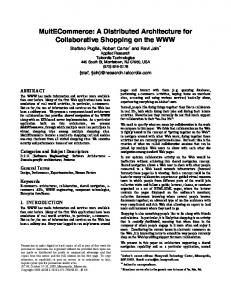
SQL interface
SQL interface Provider 1
User/App
Client (Trusted)
������������� ���������������������������������� ������������� ���� ���� ���� ���� Provider 2
SQL Queries Answers
Figure 1: The System Architecture and describes how queries may be transformed, optimized and executed in a privacy-preserving fashion. Section 5 discusses how one may design the database schema in order to minimize the execution cost of a given query workload, while obeying the constraints imposed by the needs of data privacy.
2
General Architecture
The general architecture of a distributed secure database service, as illustrated in Figure 1, consists of a trusted client as well as two or more servers that provide a database service. The servers provide reliable content storage and data management but are not trusted by the client to preserve content privacy. The client wants to out-source the (high) costs of managing permanent storage to the service providers; hence, we assume that the client does not store any persistent data. However, the client has access to cheap hardware – providing processing power as well as temporary storage – which is used to provide three pieces of functionality: 1. Offer a DBMS Front-End The client exports a standard DBMS front-end to client-side applications, supporting standard SQL APIs. 2. Reformulate and Optimize Queries The queries received by the client need to be translated into appropriate SQL sub-queries to be sent to the servers; such translation may involve limited forms of query-optimization logic, as we discuss later in the paper. 3. Post-process Query Results The sub-queries are sent to the servers (using a standard SQL API), and the results are gathered and post-processed before being returned in a suitable form to the client-side application. We note that all three pieces of functionality are fairly cheap, at least if the amount of post-processing required for queries is limited, and can be performed using inexpensive hardware, without the need for expensive data management infrastructure or personnel. Security Model As mentioned earlier, the client does not trust either server to preserve data privacy. Each
server is honest, but potentially curious: the server may actively monitor all the data that it stores, as well as the queries it receives from the client, in the hope of breaching privacy; it does not, however, act maliciously by providing erroneous service to the client or by altering the stored data. The client maintains separate, permanent channels of communication to each server. We do not require communication to be encrypted; however, we assume that no eavesdropper is capable of listening in on both communication channels. The two servers are assumed to be unable to communicate directly with each other (depicted by the “wall” between them in Figure 1) and, in fact, need not even be aware of each other’s existence. Note that the client side is assumed to be completely trusted and secure. There would not be much point in developing a secure database service if a hacker can simply penetrate the client side and transparently access the database. Preventing client-side breaches is a traditional security problem unrelated to privacy-preserving data storage, and we do not concern ourselves with this problem here. 2.1
Relation Decomposition
We now consider different techniques to partition data across the two servers in the distributed architecture described above. Say the client needs to support queries over the “universal” relation R(A1 , A2 , . . . , An ). Since the client itself possesses no permanent storage, the contents of relation R need to be decomposed and stored across the two servers. We require that the decomposition be both lossless and privacy preserving. A lossless decomposition is simply one in which it is possible to reconstruct the original relation R using only the contents in the two servers S1 and S2 . The exact manner in which such a reconstruction is performed is flexible, and may involve not only traditional relational operators such as joins and unions, but also other user-defined functions, as we discuss shortly. We also require the decomposition to be privacy preserving: the contents stored at server S1 or S2 must not, in themselves, reveal any private information about R. We postpone our discussion of what constitutes private information to the next section. Traditional relation decomposition in distributed databases is of two types: Horizontal Fragmentation Each tuple of the relation R is stored at S1 or S2 . Thus, server S1 contains a relation R1 , and S2 contains a relation R2 such that R = R 1 ∪ R2 . Vertical Fragmentation The attributes of relation R are partitioned across S1 and S2 . The key attributes are stored at both sites to ensure lossless decomposition. Optionally, other attributes may also be repli-
cated at both sites in order to improve query performance. If the relations at S1 and S2 are R1 and R2 respectively, then R = R1 ./ R2 , where ./ refers to the natural join on all common attributes. We believe that horizontal fragmentation is of limited use in enabling privacy-preserving decomposition. For example, a company might potentially store its American sales records as R1 and its European records as R2 to prevent an adversary from gathering statistics about overall sales, thus providing a crude form of privacy. In this paper, we will focus on vertical fragmentation which appears to hold much more promise. We now discuss a variety of extensions to vertical fragmentation which all aid in making the decomposition privacy preserving. Unique Tuple IDs Vertical partitioning requires a key to be present in both databases in order to ensure lossless decomposition. Since key attributes may themselves be private (and can therefore not be stored in the clear), we may introduce a unique tuple ID for each tuple and replicate this tuple ID alone across the two sites. (This concept is not new. Tuple IDs have been considered as an alternative to key replication to lower update costs in distributed databases [OV99].) There are a variety of ways to generate unique tuple IDs when inserting new tuples. Tuple IDs could simply be sequence numbers generated independently at the two servers with each new tuple insertion; so long as the client ensures that tuple insertions are atomic, both servers will automatically generate the same sequence number for corresponding tuples. Alternatively, the client could generate random numbers as tuple IDs, potentially performing a query to a server to make sure that the tuple ID does not already exist. Semantic Attribute Decomposition It may be useful to split an attribute A into two separate, but related, attributes A1 and A2 , in order to exploit privacy constraints that may apply to A1 but not to A2 . To illustrate, consider an attribute representing people’s telephone numbers. The area code of a person’s number may be sufficiently harmless to be considered public information, but the phone number, in its entirety, is information subject to misuse and should be kept private. In such a case, we may decompose the phone-number attribute into two: a private attribute A1 representing the last seven digits of the phone number, and a public attribute A2 representing the first three digits. We can immediately see the benefits of such attribute decomposition. Selection queries based on phone numbers, or queries that perform aggregation when grouping by area code, could benefit greatly from the availability of attribute A2 . In contrast, in the absence of A2 , and if the phone numbers were completely hidden (e.g., by encryption), query processing becomes more expensive.
Attribute Encoding It may be necessary to encode an attribute value across both databases so that neither database can deduce the value. For example, consider an attribute that needs to be kept private, say the employee salary. We may encode the salary attribute A as two separate attributes A1 and A2 , to be stored in the two databases. The encoding of a salary value a as two separate values a1 and a2 may be performed in different fashions, three of which we outline here: 1. One-time Pad: a1 = a random value;
L
r, a2 = r, where r is a
2. Deterministic Encryption: a1 = E(a, k), a2 = k, where E is a deterministic encryption function such as AES or RSA; 3. Random Addition: a1 = a + r, a2 = r, where r is a random number drawn from a domain much larger than that of a. In all the above cases, observe that we may reconstruct the original value of a using the values a1 and a2 . The three different encoding schemes above offer different trade-offs between privacy and efficiency. The first scheme offers true information-theoretic privacy, since both a1 and a2 consist of random bits that reveal no information about a1 . It also offers fast reconstruction of a from a1 and a2 , since only a XOR is required. However, such an encoding rules out any hope of “pushing down” a selection condition on attribute A; such conditions can be evaluated only on the client side, after fetching all corresponding a1 and a2 values from the servers and reconstructing value a. The second scheme offers no benefits over the first if the key k is chosen to be an independent random value for each tuple. However, one could use the same key k for all tuples, i.e., all values for attribute A2 are equal to the same key k. In such a case, we may be able to execute selection conditions on A more efficiently by pushing down a condition on A1 . Consider the selection condition σA=v . We may evaluate this condition efficiently as follows, assuming key k is stored at S2 :
allowing database S1 to deduce that the two tuples correspond to individuals with identical salaries. A second drawback of the scheme is that it requires encryption and decryption of attribute values at the client side which may be computationally expensive. Finally, such an encryption scheme does not help if the selection condition is a range predicate on the attribute rather than an equality predicate. The third scheme outlined above is useful when handling queries that perform aggregation on attribute A. For example, a query that requires the average salary of employees may be answered by obtaining the average of attribute A1 from database S1 , and subtracting out the average of attribute A2 from database S2 . The price paid for this efficiency is once again a compromise of true privacy: in theory, it is possible for database S1 to guess whether the salary value in a particular tuple is higher than that in another tuple. Adding Noise Another technique for enabling privacy is the addition of “noise” tuples to both databases S1 and S2 in order to improve privacy. Recall that the actual relation R is constructed by the natural join of R1 and R2 . We may thus add “dangling tuples” to both R1 and R2 without compromising the lossless decomposition property. The addition of such noise may help provide privacy, say by guaranteeing that the probability of any set of attribute values being part of a “real” tuple is less than a desired constant.
3
Defining the Privacy Requirements and Achieving It
However, a drawback of such an encoding scheme is a loss in privacy. For example, if two different tuples have the same value in attribute A, they will also possess the same encrypted value in attribute A1 , thus
So far, we have not stated the exact requirements of data privacy. There are many different formulations of data privacy, some of which are harder to achieve than others, e.g., [AS00, Swe02]. We introduce one particular definition that we believe is appropriate for the database-service context. We refer the reader to Appendix A to see how our definition captures privacy requirements imposed in legislation such as California bill SB1386 [SB02]. Our privacy requirements are specified as a set of privacy constraints P, expressed on the schema of relation R2 . Each privacy constraint is represented by a subset, say P , of the attributes of R, and informally means the following: Let R be decomposed into R1 and R2 , and let an adversary have access to the entire contents of either R1 or R2 . For every tuple in R, the value of at least one of the attributes in P must be completely opaque to the adversary, i.e., the adversary should be unable to infer anything about the value of that attribute. Note that it is permissible for the values of some attributes in P to be open, so long as there is at least
1 We assume that attribute A is of fixed length. Variablelength attributes may leak information about the length of the value unless encoded as fixed-length.
2 Other notions of privacy, such as k-anonymity [Swe02], are defined on the actual relation instances and may be harder to enforce in an efficient fashion.
1. Fetch key k from database S2 . 2. Send selection condition σA1 =E(v,k) to database S1 . 3. Obtain matching tuples from S1 .
one attribute completely hidden from the adversary. We illustrate this definition by an example. Consider a company desiring to store relation R consisting of the following attributes of employees: Name, Date of Birth (DoB), Gender, Zipcode, Position, Salary, Email, Telephone. The company may have the following considerations about privacy: 1. Telephone and Email are sensitive information subject to misuse, even on their own. Therefore both these attributes form singleton privacy constraints and cannot be stored in the clear under any circumstances. 2. Salary, Position and DoB are considered private details of individuals, and so cannot be stored together with an individual’s name in the clear. Therefore, the sets {Name, Salary}, {Name, Position} and {Name, DoB} are all privacy constraints. 3. The set of attributes {DoB, Gender, Zipcode} can help identify a person in conjunction with other publicly available data. Since we already stated that {Name, DoB} is a privacy constraint, we also need to add {DoB, Gender, Zipcode} as a privacy constraint. 4. We may also want to prevent an adversary from learning sensitive association rules, for example, between position and salary, or between age and salary. Therefore, we may add two privacy constraints: {Position, Salary}, {Salary, DoB}. What does it mean to not be able to “infer the value” of an attribute A? We have left this definition intentionally vague to accommodate the requirements of different applications. On one end, we may require true information-theoretic privacy – the adversary must be unable to gain any information about the value of the attribute from examining the contents of either R1 or R2 . We may also settle for weaker forms of privacy, such as the one provided by encoding an attribute using encryption or random addition. Neither of these schemes provides true information-theoretic privacy as above, but may be sufficient in practice. In this paper, we will restrict ourselves to the stricter notion of privacy, noting the advantages of the weaker forms where appropriate. 3.1
Obtaining Privacy via Decompositions
Let us consider how we might decompose data, using the methodologies outlined in Section 2, into two relations R1 and R2 so as to obey a given set of privacy constraints. We will restrict ourselves to the case where R1 and R2 are obtained by vertical fragmentation of R, fragmented by unique tuple IDs, with some of the attributes possibly being encoded. (We ignore
semantic attribute decomposition, as well as the addition of noise tuples. The former may be assumed to have been applied beforehand, while the latter is not useful for obeying our privacy constraints.) We abuse notation by allowing R to refer to the set of attributes in the relation. We may then denote a decomposition of R as D(R) = hR1 , R2 , Ei, where R1 and R2 are the sets of attributes in the two fragments, and E refers to the set of attributes that are encoded (using one of the schemes outlined in Section 2.1). Note that R1 ∪ R2 = R, E ⊆ R1 , and E ⊆ R2 , since encoded attributes are stored in both fragments. We denote the privacy constraints P as a set of subsets of R, i.e., P ⊆ 2R . From our definition of privacy constraints, we may state the following requirement for a privacypreserving decomposition: The decomposition D(R) is said to obey the privacy constraints P if, for every P ∈ P, P (R1 − E) and P (R2 − E). To understand how to obtain such a decomposition, we observe that each privacy constraint P may be obeyed in two ways: 1. Ensure that P is not contained in either R1 or R2 , using vertical fragmentation. For example, the privacy constraint {Name, Salary} may be obeyed by placing Name in R1 and Salary in R2 . 2. Encode at least one of the attributes in P . For example, a different way to obey the privacy constraint {Name, Salary} would be to use, say, a one-time pad to encode Salary across R1 and R2 . Observe that such encoding is the only way to obey the privacy constraint on singleton sets. Example Let us return to our earlier example and see how we may find a decomposition satisfying all the privacy constraints. We observe that both Email and Telephone are singleton privacy constraints; the only way to tackle them is to encode both these attributes. The constraints specified in items (2) and (3) may be tackled by vertical fragmentation of the attributes, e.g., R1 (ID, Name, Gender, Zipcode), and R2 (ID, Position, Salary, DoB), with Email and Telephone being stored in both R1 and R2 . Such a partitioning satisfies the privacy constraints outlined in item (2) since Name is in R1 while Salary, Position and DoB are in R2 . It also satisfies the constraint in item (3), since DoB is separated from Gender and Zipcode. However, we are still stuck with the constraints in item (4) which dictate that Salary cannot be stored with either Position or DoB. We cannot fix the problem by moving Salary to R1 since that would violate the constraint of item (2) by placing Name and Salary together.
The solution is to resort to encoding Salary across both databases. Thus, the resulting decomposition is R1 ={ID, Name, Gender, Zipcode, Salary, Email, Telephone}, R2 = {ID, Position, DoB, Salary, Email, Telephone} and E = {Salary, Email, Telephone}. Such a decomposition obeys all the stated privacy constraints. Identifying the Best Decomposition It is clear by now that it is always possible to obtain a decomposition of attributes that obeys all the privacy constraints – in the worst case, we could encode all the attributes to obey all possible privacy constraints. A key question that remains is: What is the best decomposition to use, where “best” refers to the decomposition that minimizes the cost of the workload being executed against the database? An answer to the above question requires us to understand two issues. First, we need to know how an arbitrary query on the original relation R is transformed, optimized and executed using the two fragments R1 and R2 . We will address this issue in the next section. We will then consider how to exploit this knowledge in formulating an optimization problem to find the best decomposition in Section 5.
4
Query Reformulation, Optimization and Execution
In this section, we discuss how a SQL query on relation R is reformulated and optimized by the client as subqueries on R1 and R2 , and how the results are combined to produce the answer to the original query. For the most part, it turns out that simple generalizations of standard database optimization techniques suffice to solve our problems. In Sections 4.1 and 4.2, we explain how to repurpose the well-understood distributeddatabase optimization techniques [OV99] for use in our context. We discuss the privacy implications of query execution in Section 4.3 and present some open issues in query optimization in Section 4.4. 4.1
Query Reformulation
Query reformulation is straightforward and identical to that in distributed databases. Consider a typical conjunctive query that applies a conjunction of selection conditions C to R, groups the results using a set of attributes G, and applies an aggregation function to a set of attributes A. We may translate the logical query plan of this query into a query on R1 and R2 by the following simple expedient: replace R by R1 ./ R2 (with the understanding that the ./ operation also replaces encoded pairs of attribute values with the unencoded value). When the query involves a self-join on R, we simply replace each occurrence of R by the above-mentioned join3 . 3 Note that since R is considered to be the universal relation, all joins are self-joins.
Figure 2 shows how a typical query involving selections and projections on R (part (a) of figure) is reformulated as a join query on R1 and R2 (part (b) of figure). 4.2
Query Optimization
The trivial query plan for answering a query reformulated in the above fashion is as follows: Fetch R1 from S1 , fetch R2 from S2 , execute all plan operators locally at the client. Of course, such a plan is extremely expensive, as it requires reading and transmitting entire relations across the network. Optimizing the Logical Query Plan The logical query plan is first improved, just as in traditional query optimization, by “pushing down” selection conditions, with minor modifications to account for attribute fragmentation. Consider a selection condition c: • If c is of the form hAttri hopi hvaluei, and hAttri has not undergone attribute fragmentation, condition c may be pushed down to R1 or R2 , whichever contains hAttri. (In case hAttri is replicated on both relations, the condition may be pushed down to both.) • If c is of the form hAttr1i hopi hAttr2i, and both hAttr1i and hAttr2i are unfragmented and present in either R1 or R2 , the condition may be pushed down to the appropriate relation. Similarly, projections may also be pushed down to both relations, taking care not to project out tuple IDs necessary for the join. Group-by clauses and aggregates may also pushed down, provided all attributes mentioned in the Group-by and aggregate are unfragmented and present together in either R1 or R2 . Selfjoins of R with itself, translated into four-way joins involving two copies each of R1 and R2 , may be rearranged to form a “bushy” join tree where the two R1 copies, and the two R2 copies, are joined first. Figure 2(c) shows the pushing down of selections and projections to alter the logical query plan. We assume attributes are fragmented as in the example of Section 3: R1 contains Name, while DoB is in R2 and Salary is encoded across both relations. Thus, the condition on Name is pushed down to R1 , while the condition on DoB is pushed down to R2 . The selection on Salary cannot be pushed down since Salary is encoded. In addition, we may push down projections as shown in the figure. Choosing the Physical Query Plan Having optimized the logical query plan, the physical plan needs to be chosen, determining how the query execution is partitioned across the two servers and the client. The basic partitioning of the query plan is straightforward: all operators present above the top-most join have to
Client
π N ame
π
σ
N ame
π N ame
Salary > 80K
σ
σ DoB > 1970∧ N ame LIKE 0 Bob0 ∧ Salary > 80K
DoB > 1970∧ N ame LIKE 0 Bob0 ∧ Salary > 80K
Site 1
./
π
π
ID, N ame, Salary
ID, Salary
./ σ
R R2
R1
σ
N ame LIKE 0 Bob0
R1 (a)
Site 2
(b)
DoB > 1970
R2 (c)
Figure 2: Example of Query Reformulation and Optimization be executed on the client side; all operators underneath the join and above Ri are executed by a subquery at server Si for i = 1, 2 (shown by the dashed boxes in Figure 2). In the ideal case, it may be possible to push all operators to one of R1 or R2 , eliminating the need for a join. Otherwise, we are left with a choice in deciding how to perform the join. The first option is to send sub-queries to both S1 and S2 in parallel, and join the results at the client. The second option is to send only one of the two subqueries, say to server S1 ; the tuple IDs of the results obtained from S1 are then used to perform a semi-join with the content on server S2 , in addition to applying the S2 -subquery to filter R2 . To illustrate with the example of Figure 2(c), consider the following two sub-queries: Q1 : SELECT Name, ID, Salary FROM R1 WHERE (Name LIKE Bob) Q2 : SELECT ID, Salary FROM R2 WHERE (DoB > 1970) There are then three options available to the client for executing the query: 1. Send sub-query Q1 to S1 , send Q2 to S2 , join the results on ID at the client, and apply the selection on Salary. 2. Send sub-query Q1 to S1 . Apply πID to the results of Q1 ; call the resulting set Λ. Send S2 the query Q3 : SELECT ID, Position, Salary FROM R2 WHERE (ID IN Λ) AND (DoB > 1970). Join the results of Q3 with the results of Q1 . 3. Send sub-query Q2 to S2 . Apply πID to the results of Q2 and rewrite Q1 in an analogous fashion
to the previous case. The first plan may be expensive, since it requires a lot of data to be transmitted from site S2 . The second plan is potentially a lot more efficient, since only tuples that match the condition Name LIKE Bob are ever transmitted from both S1 and S2 . However, there may be a greater delay in obtaining query answers; the results from S1 need to be obtained before a query is sent to S2 . In our example, the third plan is unlikely to be efficient unless the company consists only of old people. We illustrate query optimization with two more examples. Example 2 Consider the query: SELECT SUM(Salary) FROM R Say Salary is encoded using Random Addition instead of by a one-time pad. In this case, the client may simultaneously issue two subqueries: Q1 : SELECT SUM(Salary) FROM R1 Q2 : SELECT SUM(Salary) FROM R2 The client then computes the difference between the results of Q1 and Q2 as the answer. Example 3 Consider the query: SELECT Name FROM R WHERE DoB> 1970 AND Gender=M The client first issues the following sub-query to S2 : Q2 : SELECT ID FROM R2 WHERE DoB> 1970 After it gets the ID list Λ from Q2 , it sends S1 the query: SELECT Name FROM R1 WHERE Gender=M AND ID in Λ. Note that the alternative plan – sending sub-queries in parallel to both S1 and S2 – may be more efficient if the condition DoB> 1970 is highly unselective.
4.3
Query Execution and Data Privacy
One question that may arise from our discussion of query execution is: Is it possible for an adversary monitoring activity at either S1 or S2 to breach privacy by viewing the queries received at either of the two databases? We claim that the answer is ‘No’. Observe that when using simple joins as the query plan, the subqueries sent to S1 and S2 are dependent only on the original query and not on the data stored at either location; thus, the sub-queries do not form a “covert channel” by which information about the content at S1 could potentially be transmitted to S2 or vice versa. However, when semi-joins are used, we observe that the query sent to S2 is influenced by the results of the sub-query sent to S1 . Therefore, a legitimate concern might be that the sub-query sent to S2 leaks information about the content stored at S1 . We avoid privacy breaches in this case by ensuring that only tuple IDs are carried over from the results of S1 into the query sent to S2 . Since knowledge of some tuple IDs being present in S1 does not help an adversary at S2 in inferring anything about other attribute values, such a query execution plan continues to preserve privacy. 4.4
Discussion
The above discussion does not by any means exhaust all query-optimization issues in the two-server context. We now list some areas for future work, with preliminary observations about potential solutions. Maintaining Statistics for Optimization Our discussion of the space of query plans implicitly assumed that the client has sufficient database statistics at hand, and a sufficiently good cost model, for it to choose the best possible plan for the query. More work is required to validate both the above assumptions. For example, one question is to understand where the client obtains its statistics from. Statistics on the individual relations R1 and R2 could be obtained directly from the servers S1 and S2 . The statistics may be cached on the client side in order to avoid having to fetch them from the servers for each optimization. There may potentially be statistics, e.g., multi-dimensional histograms, that require knowledge of both relations R1 and R2 in order to be maintained. If necessary, such statistics could conceivably be maintained on the client side and may be constructed by means of appropriate SQL sub-queries sent to the two servers. Supporting Other Decomposition Techniques Our discussion of query optimization so far has only covered the case of vertical fragmentation with attribute encoding using one-time pads or random addition. It is possible to optimize the query plans further when performing attribute encoding by deterministic
encryption, or when using semantic attribute decomposition. For example, when an attribute is encrypted by a deterministic encryption function, it is possible to push down selection conditions of the form hattri = hconsti, by obtaining the encryption key from one database and encrypting hconsti with this key before pushing down the condition. When an attribute is decomposed by semantic decomposition, the resulting functional dependencies across the decomposed attributes may potentially be used to push down additional selection conditions. To illustrate, consider a PhoneNumber (PN) attribute which is decomposed into AreaCode (AC) and LocalNumber(LN). A selection condition of the form σP N =5551234567 could still be pushed down partially as σAC=555 and σLN =1234567 . (Note that the original condition cannot be eliminated, and still needs to be applied as a filter at the end.) Such rewriting depends on the nature of the semantic decomposition; the automatic application of such rewriting therefore requires support for specifying the relationship between attributes in a simple fashion.
5
Identifying the Optimal Decomposition
Having seen how queries may be executed over a decomposed database, our next task at hand is to identify the best decomposition that minimizes query costs. Say, a workload W consisting of the actual queries to be executed on R is available. We may then think of the following brute-force approach: For each possible decomposition of R that obeys the privacy constraints P: • Optimize each query in W for that decomposition of R, and • Estimate the total cost of executing all queries in W using the optimized query plans. We may then select that decomposition which offers the lowest overall query cost. Observe that such an approach could be prohibitively expensive, since there may be an extremely large number of legitimate decompositions to consider, against each of which we need to evaluate the cost of executing all queries in the workload. To work around this difficulty, we attempt to capture the effects of different decompositions on query costs in a more structured fashion, so that we may efficiently prune the space of all decompositions without actually having to evaluate each decomposition independently. A standard framework to capture the costs of different decompositions, for a given workload W , is the notion of the affinity matrix [OV99] M , which we adopt and generalize as follows:
1. The entry Mij represents the “cost” of placing the unencoded attributes i and j in different fragments. 2. The entry Mii represents the “cost” of encoding attribute i across both fragments. We assume that the cost of a decomposition may be expressed simply by a linear combination of entries in the affinity matrix. Let R = {A1 , A2 , . . . An } represents the original set of n attributes, and consider a decomposition of D(R) = hR1 , R2 , Ei. Then, weP assume that the cost of this Pdecomposition C(D) is M + ij i∈(R1 −E),j∈(R2 −E) i∈E Mii . ( For simplicity, we do not consider replicating any unencoded attribute, other than the tupleID, at both sites.) In other words, we add up all matrix entries corresponding to pairs of attributes that are separated by fragmentation, as well as diagonal entries corresponding to encoded attributes, and consider this sum to be the cost of the decomposition. Given this simple model of the cost of decompositions, we may now define an optimization problem to identify the best decomposition: Given a set of privacy constraints P ⊆ 2R and an affinity matrix M , find a decomposition D(R) = hR1 , R2 , Ei such that (a) P D obeys all privacy constraints Pin P, and (c) i,j:i∈(R1 −E),j∈(R2 −E) Mij + i∈E Mi is minimized. We are left with two questions: • How is the affinity matrix M generated from a knowledge of the query workload? • How can we solve the optimization problem? We address the first question in Appendix B, where we present heuristics for generating the affinity matrix. We discuss the second question next. 5.1
Solving the Optimization Problem
We may define our optimization problem as the following hypergraph-coloring problem: We are given a complete graph G(R), with both vertex and edge weights defined by the affinity matrix M . (Diagonal entries stand for vertex weights.) We are also given a set of privacy constraints P ⊆ 2R , representing a hypergraph H(R, P) on the same vertices. We require a 2-coloring of the vertices in R such that (a) no hypergraph edge in H is monochromatic, and (b) the weight of bichromatic graph edges in G is minimized. The twist is that we are allowed to delete any vertex in R (and all hyperedges in P that contain the vertex) by paying a price equal to the vertex weight.
Observe that coloring a vertex is equivalent to placing it in one of the two partitions. Deleting the vertex is equivalent to encoding the attribute; so, all privacy constraints associated with that attribute are satisfied by the vertex deletion. Also observe that vertex deletion may be necessary, since it is not always possible to 2-color a hypergraph. The above problem is very hard to solve – even if we remove the feature of vertex deletion (allowing encoding), say by guaranteeing that the hypergraph is 2colorable. In fact, much more restrictive special cases are NP-hard, even to approximate, as the following result shows: It is NP-hard to color a 2-colorable, 4uniform hypergraph using only c colors for any constant c [GHS00]. In other words, even if all privacy constraints were 4-tuples of attributes, and it is known that there exists a partitioning of attributes into two sets that satisfies all constraints, it is NP-hard to partition the attributes into any fixed number of sets, let alone two, to satisfy all the constraints! Given the hardness of the hypergraph-coloring problem, we consider three different heuristics to solve our optimization problem. All our heuristics utilize the following two solution components: Approximate Min-Cuts If we were to ignore the privacy constraints for a moment, observe that the resulting problem is to two-color the vertices to minimize the weight of bichromatic edges in G(R); this is equivalent to finding the min-cut in G (assuming that at least one vertex needs to be of each of the two colors). This problem can be solved optimally in polynomial time, but we will be interested in a slightly more general version: We will require all cuts of the graph that have a weight within a specified constant factor of the min-cut. Intuitively, we want to produce a lot of cuts that are near-optimal in terms of their quality, and we will choose among the cuts to pick one that helps satisfy the most privacy constraints. This approximate mincut problem can still be solved efficiently in polynomial time using an algorithm based on edge contraction [KS96]. (Note that this also implies that the number of cuts produced by the algorithm is only polynomially large.) Approximate Weighted Set Cover Our second component uses a well-known tool in order to tackle the satisfaction of the privacy constraints via vertex deletion. Let us ignore the coloring problem and consider the following problem instead: Find the minimum weight choice of vertices to delete so that all hypergraph edges are removed, i.e., each set P ∈ P loses at least one vertex. This is the minimum weighted set-cover problem, and the best known solution is to use the following
greedy strategy: keep deleting the vertex that has the lowest cost per additional set that it covers, until all sets are covered. This greedy strategy offers a (1 + log |P|)-approximation to the optimal solution [Joh73, Chv79] and will be used by us in our heuristics. We now present three different heuristics which utilize the above two components: Heuristic 1 Our first heuristic is to solve the optimization problem in three phases: 1. Ignore fragmentation, and delete vertices to cover all the constraints using Approximate Weighted Set Cover. Call the set of deleted vertices E. 2. Consider the remaining vertices, and use Approximate Min-Cuts to find different 2colorings of the vertices, all of which approximately minimize the weight of the bichromatic edges in G. 3. For each of the 2-colorings obtained in step (2): Find all deleted vertices that are present only in bichromatic hyperedges, and consider “rolling back” their deletion, and coloring them instead, to obtain a better solution. 4. Choose the best of (a) the solution from step (3) for each of the 2-colorings, and (b) the decomposition hR − E, E, Ei. In the first step, we cover all the privacy constraints by ensuring that at least one attribute in each constraint is encoded. Note that this step leads us directly to one possible decomposition: place all deleted vertices in both fragments, and all the remaining vertices in one of the two fragments. Call this decomposition D1 . In the next two steps, we attempt to improve on D1 by avoiding encrypting all these attributes, hoping to use fragmentation to cover some of the constraints instead. To this end, we find different approximate mincuts in step (2), each of which fragments the attributes differently. In each fragmentation, we try to roll back some of the attribute encoding (vertex deletion) that had earlier been necessary to cover some constraints, but is no longer needed thanks to the fragmentation satisfying the constraints instead. Finally, we compare the quality of the different solutions obtained from step (3), with the basic solution D1 obtained directly from step 1, and select the best of the lot. Note that the entire heuristic runs in polynomial time, because the number of different cuts considered is only a polynomial function of |R|. Heuristic 2 Our second heuristic reverses the order in which fragmentation (2-coloring) and encoding (deletion) are attempted. We first apply Approximate Min-Cuts to the original graph G(R) to obtain a set
of possible cuts. For each such cut, we perform the following steps: (a) Some of the privacy constraints are already satisfied by the fragmentation; we therefore delete these constraints from P, (b) We apply Approximate Weighted Set Cover to the modified P, deleting vertices until all constraints are satisfied. Finally, we may once again compare the solutions obtained from each cut and select the best one. Heuristic 3 The third approach we consider is to interleave the execution of our approximate min-cut and set-cover components, instead of just using one after the other. We start with some 2-coloring obtained by running Approximate Min-cuts. We then repeat the following steps until all constraints are satisfied: 1. Use Approximate Set Cover to greedily select one vertex to delete. (Note that we only delete one vertex, instead of deleting as many as necessary to satisfy all constraints.) 2. Having deleted this vertex, re-run Approximate Min-Cuts and attempt to find a 2-coloring that satisfies even more constraints than the current coloring. (If we can’t find such a coloring, retain the current coloring.) Observe that the above heuristic uses many more invocations of the min-cut algorithm in order to recompute colorings after each vertex deletion. To obtain some intuition as to why this heuristic is useful, consider some vertex v which has high-weight graph edges to some of its neighbors v1 , v2 , . . . vk . A min-cut on the original graph will tend to force v together with all these neighbors (i.e., all these vertices will have the same color) since the edges from v to v1 , v2 , . . . vk are all of high weight. However, once v is deleted, the nature of the coloring may change dramatically; the different vertices v1 , v2 , . . . vk may no longer need to have the same color, which opens the door for colorings that can satisfy many more privacy constraints (specifically, constraints that can be satisfied by separating some of the vertices in v1 , v2 , . . . vk ). 5.2
Discussion
There are many open questions surrounding the above decomposition problem. One question is to understand the relative performance of our different design heuristics on different relation schemata and privacy constraints. Another is to develop better theoretical approaches to the optimization problem. Formulating the optimization problem itself is based on a number of heuristics (discussed in Appendix B) which are also open to improvement. The scope of the optimization problem may also be expanded in a number of different directions.
For example, we could allow attributes to be replicated across partitions, trying to exploit such replication to lower query costs. In the terminology of the optimization problem, vertices are allowed to take on both colors. Edges in G emanating from a vertex v with two colors will not be considered bichromatic; however, hyperedges involving v will need to be bichromatic even when ignoring v. Another extension is to deal with constraints imposed by functional dependencies, normal forms and multiple relations. For example, we may want our decomposition to be dependency-preserving, which dictates that functional dependencies should not be destroyed by data partitioning. Different partitioning schemes may have different impacts on the cost of checking various constraints. Factoring these issues into the optimization problem is a subject for future work. Finally, expanding the definition of the optimization problem to accommodate the space of different encoding schemes for each attribute is also an area as yet unexplored.
6
Related Work
Secure Database Services As discussed in the introduction, the outsourcing of data management has motivated the model where a DBMS provides reliable storage and efficient query execution, while not knowing the contents of the database [HIM02]. Schemes proposed so far for this model encrypt data on the client side and then store the encrypted database on the server side [HILM02, HIM04, AKSX04]. However, in order to achieve efficient query processing, all the above schemes only provide very weak notions of data privacy. In fact a server that is secure under formal cryptographic notions can be proved to be hopelessly inefficient for data processing [KC04]. Our architecture of using multiple servers helps to achieve both efficiency and provable privacy together. Trusted Computing With trusted computing [TCG03], a tamper-proof secure co-processor could be installed on the server side, which allows executing a function while hiding the function from the server. Using trusted tamper-proof hardware for enabling secure database services has been proposed in [KC04]. However, such a scheme could involve significant computational overhead due to repeated encryption and decryption at the tuple level. Understanding the role of tamper-proof hardware in our architecture remains a subject of future work. Secure Multi-party Computation Secure multiparty computation [Yao86, GMW87] discusses how to compute the output of a function whose inputs are stored at different parties, such that each party learns only the function output and nothing about the inputs of the other parties. In our context, there are two par-
ties – the server and the client – with the server’s input being encrypted data, the client’s input being the encryption key, and the function being the desired query. In principle, the client and the server could then engage in a one-sided secure computation protocol to compute the function output that is revealed only to the client. However, “in principle” is the operative phrase, as the excessive communication overhead involved makes this approach even more inefficient than the trivial scheme in which the client fetches the entire database from the server. More efficient specialized secure multi-party computation techniques have been studied recently[LP00, AMP04, FNP04]. However all of this work is to enable different organizations to securely analyze their combined data, rather than the client-server model we are interested in. Privacy-preserving Data Mining Different approaches for privacy-preserving data mining studied recently include: (1) perturbation techniques [AS00, AA01, EGS03, DN03, DN04] (2) query restriction/auditing [CO82, DJL79, KPR00] (3) k-anonymity [Swe02, MW04, AFK+ 04]. However, research here is motivated by the need to ensure individual privacy while at the same time allowing the inference of highergranularity patterns from the data. Our problem is rather different in nature, and the above techniques are not directly relevant in our context. Access Control Access control is used to control which parts of data can be accessed by different users. Several models have been proposed for specifying and enforcing access control in databases [CFMS95]. Access control does not solve the problem of maintaining an untrusted storage server as even the the administrator or an insider having complete control over the data at the server is not trusted by the client in our model.
7
Conclusions
We have introduced a new distributed architecture for enabling privacy-preserving outsourced storage of data. We demonstrated different techniques that could be used to decompose data, and explained how queries may be optimized and executed in this distributed system. We introduced a definition of privacy based on hiding sets of attribute values, demonstrated how our decomposition techniques help in achieving privacy, and considered the problem of identifying the best privacy-preserving decomposition. Given the increasing instances of database outsourcing, as well as the increasing prominence of privacy concerns as well as regulations, we expect that our architecture will prove useful both in ensuring compliance with laws and in reducing the risk of privacy breaches. A key element of future work is to test the viability of our architecture through a real-world case study. Other future work includes identifying improved al-
gorithms for decomposition, expanding the scope of techniques available for decomposition, e.g., supporting replication, and incorporation of these techniques into the query optimization framework.
[HILM02] H. Hacigumus, B. Iyer, C. Li, and S. Mehrotra. Executing sql over encrypted data in the database-service-provider model. In Proc. SIGMOD, 2002. [HIM02]
H. Hacigumus, B. Iyer, and S. Mehrotra. Providing database as a service. In Proc. ICDE, 2002.
[HIM04]
[AFK+ 04] G. Aggarwal, T. Feder, K. Kenthapadi, R. Motwani, R. Panigrahy, D. Thomas, and A. Zhu. Anonymizing tables. Technical report, Stanford University, 2004.
H. Hacigumus, B. Iyer, and S. Mehrotra. Efficient execution of aggregation queries over encrypted relational databases. In Proc. DASFAA, 2004.
[Joh73]
[AKSX04] Rakesh Agrawal, Jerry Kiernan, Ramakrishnan Srikant, and Yirong Xu. Order-preserving encryption for numeric data. In Proc. SIGMOD, 2004.
David S. Johnson. Approximation algorithms for combinatorial problems. In Proc. 5th annual ACM Symposium on Theory of Computing(STOC), 1973.
[KC04]
Murat Kantarcioglu and Chris Clifton. Security issues in querying encrypted data. Technical Report TR-04-013, Purdue University, 2004.
[AMP04]
G. Aggarwal, N. Mishra, and B. Pinkas. Secure computation of the k-th ranked element. In Proc. EUROCRYPT, 2004.
[KPR00]
Jon M. Kleinberg, Christos H. Papadimitriou, and Prabhakar Raghavan. Auditing boolean attributes. In Proc. PODS, 2000.
[AS00]
R. Agrawal and R. Srikant. Privacy-preserving data mining. In Proc. SIGMOD, 2000.
[KS96]
[CFMS95] S. Castano, M. Fugini, G. Martella, and P. Samarati. Principles of Distributed Database Systems. Addison Wesley, 1995.
David Karger and Clifford Stein. A new approach to the minimum cut problem. Journal of the ACM, 43(4):601–640, July 1996.
[LP00]
Y. Lindell and B. Pinkas. Privacy-preserving data mining. In Proc. CRYPTO, 2000.
[Chv79]
Vasek Chvatal. A greedy heuristic for the setcovering problem. Mathematics of Operations Research, 4(3):233–235, 1979.
[MW04]
A. Meyerson and R. Williams. On the complexity of optimal k-anonymity. In Proc. PODS, 2004.
[CO82]
F. Chin and G. Ozsoyoglu. Auditing and inference control in statistical databases. In IEEE TSE, 8(6), 1982.
[OV99]
M. Tamer Ozsu and Patrick Valduriez. Principles of Distributed Database Systems. Prentice Hall, 2nd edition, 1999.
[CW02]
J.P. Morgan signs outsourcing deal with IBM. ComputerWorld, Dec 30, 2002.
[DJL79]
D. Dobkin, A. Jones, and R. Lipton. Secure databases: Protection against user influence. In ACM TODS, 4(1), 1979.
[SAC+ 79] Patricia G. Selinger, Morton M. Astrahan, Donald D. Chamberlin, Raymond A. Lorie, and Thomas G. Price. Access path selection in a relational database management system. In Proc. SIGMOD, pages 23–34, 1979.
[DN03]
I. Dinur and K. Nissim. Revealing information while preserving privacy. In Proc. PODS, 2003.
[DN04]
C. Dwork and K. Nissim. Privacy-preserving datamining on vertically partitioned databases. In Proc. CRYPTO, 2004.
References [AA01]
D. Agrawal and C. Aggarwal. On the design and quantification of privacy preserving datamining algorithms. In Proc. PODS, 2001.
[SB02]
California senate bill SB 1386. http: //info.sen.ca.gov/pub/01-02/bill/sen/ sb_1351-1400/sb_1386_bill_20020926_ chaptered.html, Sept. 2002.
[Swe02]
L. Sweeney. k-Anonymity: A model for preserving privacy. In International Journal on Uncertainty, Fuzziness and Knowledge-based Systems, 10(5), 2002.
[EGS03]
A. Evfimievski, J. Gehrke, and R. Srikant. Limiting privacy breaches in privacy preserving data mining. In Proc. PODS, 2003.
[TCG03]
[FNP04]
M. Freedman, K. Nissim, and B. Pinkas. Efficient private matching and set intersection. In Proc. EUROCRYPT, 2004.
TCG TPM specification version 1.2. https://www.trustedcomputinggroup.org, Nov 2003.
[WP04]
Advertiser charged in massive database theft. The Washington Post, July 22, 2004.
[Yao86]
Andrew Yao. How to generate and exchange secrets. In Proc. FOCS, 1986.
[GHS00]
V. Guruswami, J. Hastad, and M. Sudan. Hardness of approximate hypergraph coloring. In Proc. 41st Annual Symposium on Foundations of Computer Science (FOCS), 2000.
[GMW87] O. Goldreich, S. Micali, and A. Wigderson. How to play any mental game – a completeness theorem for protocols with a honest majority. In Proc. STOC, 1987.
A
Extract from California SB 1386
The California Senate Bill SB 1386, which went into effect on July 1, 2003, defines what constitutes personal information of individuals, and mandates various procedures to be followed by state agencies and businesses in California in case of a breach of data security in that organization. We present below its definition of personal information, observing how it is captured by our definition of privacy constraints (the italics are ours): For purposes of this section, “personal information” means an individual’s first name or first initial and last name in combination with any one or more of the following data elements, when either the name or the data elements are not encrypted: (1) Social security number. (2) Driver’s license number or California Identification Card number. (3) Account number, credit or debit card number, in combination with any required security code, access code, or password that would permit access to an individual’s financial account. For purposes of this section, “personal information” does not include publicly available information that is lawfully made available to the general public from federal, state, or local government records. [SB02]
B
Computing the Affinity Matrix
Let us revisit the definition of the affinity matrix to examine its semantics: the entry Mij is required to represent the “cost” of placing attributes i and j in different partitions of a decomposition, while the entry Mii represents the “cost” of encoding attribute i, with the overall cost of decomposition being expressed as a linear combination of these entries. Note that it is likely impossible to obtain a matrix that accurately captures the costs of all decompositions. The costs of partitioning different pairs of attributes are unlikely to be independent; placing attributes i and j in different partitions may have different effects on query costs, depending on how the other attributes are placed and encoded. Our objective is to come up with simple heuristics to obtain a matrix that does a reasonable job of capturing the relative costs of different decompositions. Similar matrices are used to capture costs in other contexts too, e.g., the allocation problem in distributed databases [OV99]. Our problem is complicated somewhat by the fact that we need to account for the effects of attribute encoding on query costs, as well as the interactions between relation fragmentation and encoding.
A First Cut As a first cut, we may consider the following simple way to populate the affinity matrix from a given query workload, along the lines of earlier approaches [OV99]: • Mij is set to be the number of queries that reference both attributes i and j. • Mii is set to be the number of queries involving attribute i. Of course this simple heuristic ignores many issues: different queries in the workload may have different costs and should not be weighted equally; the effect of partitioning attributes i and j may depend on how i and j are used in the query, e.g., in a selection condition, in the projection list, etc.; the cost of encoding an attribute may be very different from that of partitioning two attributes, so that counting both on the same scale may be a poor approximation. In order to improve on this first cut, we dig deeper to understand the effects of fragmentation and encoding on query costs. B.1
The Effects of Fragmentation
Let us consider a query that involves attributes i and j and evaluate the effect of a fragmentation that separates i and j on the query. We may make the following observations: • If i and j are the only attributes referenced in the query, the fragmentation forces the query to touch both databases, and increases the communication cost for the query; the extra communication cost is proportional to the number of tuples satisfying the most selective conditions on one of the two attributes. • If attributes other than i and j are involved in the query, it is possible that the query may have to touch both databases even if i and j were held together, since the separation of other attributes may be the culprit. Therefore, the query cost that may be attributed to Mij should be only a fraction of the query overhead caused by fragmentation. • If i or j is part of a GROUP BY clause, fragmentation makes it impossible to apply the GROUP BY, making the query overhead very high. Using the above observations, we may devise a scheme to populate the matrix entries Mij for i 6= q. Each entry Mij is computed as a sum of “contributions” from each query that references both i and j. The contribution of a query Q to Mij , for any pair i and j referenced in Q, is a measure of the fraction of extra tuple fetches from disk, and transmissions across the network, that are induced by the partitioning of i and j. We define this contribution as follows: ( Let si
be the selectivity of Q, ignoring all conditions involving i, and sj be its selectivity ignoring all conditions involving j.) • If Q involves either i or j in a GROUP BY, or a selection condition, the contribution of Q to Mij is set to min(si , sj ). • If Q involves i and j only in the projection list, the contribution of Q to Mij is set to min(si , sj )/n where n is the number of attributes referenced in Q’s projection list. Note that the approach above requires the estimation of query selectivities; this may be performed using standard database techniques, i.e., using a combination of selectivity estimates from histograms, independence assumptions, and ad hoc guesses about the selectivity of predicates [SAC+ 79]. B.2
The Effects of Encoding
Let us now consider the effects of encoding attributes on query costs. We make the following observations about the effects of encoding attribute i on a query Q: (We will assume that encoding is performed using one-time pads or random addition.) • If Q contains a selection condition involving i, the condition cannot be pushed down; the overhead due to this is proportional to the selectivity of the query ignoring the conditions on i. • If Q involves i only in the projection list, there may be additional overhead equal to the cost of fetching i from both sides. • If Q involves i in the GROUP BY clause, grouping cannot be pushed down, and may cause additional overhead. • If Q involves i only as an attribute to be aggregated, the use of Random Addition for encoding ensures that the overhead of encoding is low. From these observations, we use the following rules to determine the contributions of Q to Mii : (Again, we let si be the selectivity of the query ignoring predicates involving i.) • If i is in a selection condition or a GROUP BY clause, the contribution to Mii is set to si . • Else, if i is in the projection list, the contribution to Mii is set to 1/n, where n is the total number of attributes referenced by Q.


![[PDF] Can You Keep a Secret? Full Colection - Google Sites](https://m.moam.info/img/260x300/pdf-can-you-keep-a-secret-full-colection-google-si_6477d8e2097c47a9708c2b2d.jpg)


![[PDF] Read Can You Keep a Secret? Epub - Google Sites](https://m.moam.info/img/260x300/pdf-read-can-you-keep-a-secret-epub-google-sites_647783f8097c474e708bc9cb.jpg)