two dimensional computational modelling of flow in polgolla reservoir ...

The 28th International Symposium on Transport Phenomena 22-24 September 2017, Peradeniya, Sri Lanka

TWO DIMENSIONAL COMPUTATIONAL MODELLING OF FLOW IN POLGOLLA RESERVOIR L.M.L.K.B.Lindamulla1, D.M.S.B. Dissawa1 and S.B. Weerakoon 1 1

Department of Civil Engineering, Faculty of Engineering, University of Peradeniya, Peradeniya, Sri Lanka

ABSTRACT Sediment accumulation is identified to be a major problem faced by most of the reservoirs around the world. Operations of Polgolla reservoir is recognized to have threatened seriously due to sedimentation. Therefore sediment removal is necessary. At Polgolla reservoir this is done by sluicing. This study was carried out to identify the best gate opening combination for sluicing the sediment from Polgolla reservoir. Efficiency of sluicing can be optimised by having clear understanding on the flow pattern at different discharges and different combinations of gate openings. A two dimensional depth averaged computational model was developed to the Polgolla reservoir using “SToRM” module of iRIC modelling software. Flow computation is based on Saint-Venant equations of channel flow. Considering the bathymetry of the reservoir, an unstructured grid system covering the reservoir area was generated using iRIC interface. Generated grid system was simulated with upstream discharges and downstream wáter level as the bounary conditions. Then the model was calibrated with set of field measurements and another set of field measurements at selected sections were used to validate the generated model. Eight different inflow and gate opening combinations were simulated using the model and flow patterns were observed. From the results obtained from the simulations, opening of middle gates during high discharges gave flow patterns which can sluice out sediment efficiently. Further the generated iRIC pro model can be used to simulate different scenarios and predict water depths, flow velocity, discharge as well.

INTRODUCTION Sediment accumulation is one of the main problem in reservoirs. Storage capacity of reservoirs across the world is reducing due to sediment deposition and therefore sediment management is important for sustaining the useful life of reservoirs (Neena et al., 2014). Benefits expected out of water resource projects often fall short due to sedimentation in reservoirs. It has impacts on hydropower production, irrigation water supply, extra cost on water purification and loss of fishery yields (Herath & Chennat, 1999). Continuing reduction in water capacity with reservoir siltation is now recognized as one of the biggest threat in almost all the reservoirs of Sri Lanka. The results of preliminary investigations carried out by British-ODA in upper Mahaweli watershed has showed that not only the reservoir capacity is reducing but also the rate of siltation has increased (Wickramasinghe, 1995).

Sediment accumulation in Polgolla reservoir is identified as a serious problem for its operations. Reservoir storage capacity is reducing gradually with increasing rate and therefore sediment removal is necessary. It is done by sluicing through gates. Having a clear understanding on the flow pattern for different combinations of discharges and gate openings will help in efficient sluicing of sediment from the reservoir. Sluicing can be effectively applied for the sediment removal from reservoirs. Substantial quantity of sediment can be removed and reservoir storage capacity can be restored by proper planning and execution of flushing. Simulation of flow in reservoirs helps in optimizing the sluicing operation. Therefore modelling of flow pattern and flow velocity is useful in operating the reservoirs. Flow modelling can be done either physically or computationally. Physical modelling has its limitations over computational modelling (Downs et al., 2009). Computational modelling of flow also can be sub divided into multi-dimensional modelling as one dimensional flow modelling, two dimensional flow modelling (Ahmad & Simonovic, 1999) and three dimensional flow modelling (Schleiss et al.,2014). The models most commonly used for the computation of shallow water flows solve either the 3D shallow water equations or the 2D shallow water equations (Luis et al., 2007). Shallow water flows are those in which the vertical characteristic length scale is much smaller than the horizontal one (Yuce & Chen 2003). Shallow water reservoirs such as Polgolla can be modelled efficiently and up to a satisfactory level of accuracy using 2D modelling approach. For the computation process modelling packages will require reservoir bathymetry, existing water level, inflow outflow data, bed shear stress etc. (Morianou et al., 2015). The model can be calibrated and validated against field measured velocities (Jeyakaran et al. 2015). The resulting model can be then used for future forecasting of flow velocities and to monitor the sediment flushing from reservoir. In this research, flow pattern in Polgolla reservoir was modelled. A two dimensional computational model, iRIC was used for the purpose of modelling. Necessary data for the modelling of the flow was collected from relevant sources. Applying gathered data, the grid of the reservoir was generated and using iRIC software flow was modelled. Using measured flow velocities and depths, generated model was calibrated and verified. Finally it was applied to Polgolla Reservoir considering different inflow values and different gate openings.

The 28th International Symposium on Transport Phenomena 22-24 September 2017, Peradeniya, Sri Lanka

STUDY AREA The study area was focused to Polgolla reservoir extending from Gatambe to barrage at Polgolla Special attention was provided to area closer to the barrages as flow pattern identification at the barrage site is of more importance. Polgolla barrage is a weir constructed to divert the Mahaweli river water mainly for irrigation purposes. Sudu Ganga carries the diverted water to the North Central Province. And part of water is utilized for electricity generation at Ukuwela hydro power plant. Water flowing along the Mahaweli River passes through Victoria, Randenigala and Rantembe dams generating of electricity. Polgolla reservoir, the first project under Mahaweli development project, started construction in 1970 and completed and started its operations in 1976. The reservoir is of gross capacity of 4.1 MCM with maximum length of 1.2 km and maximum width of 170 m. The barrage is 144 m in length and 14.6 m in height. There are 10 steel roller gates with clear span of 12.2 m. Each gate is of a total height of 6.4 m comprising of upper gate of 3.3 m and lower gate 3.1 m. The barrage is designed for a head of 21 m. GOVERNING EQUATIONS

(8)

(9) Where; h is water depth t is time u and v are depth-averaged velocities in x- and ydirections g is gravitational acceleration H is water depth and are the components of the shear stress of river bed in x- and y directions Fx and Fy are components of drag force by vegetation in the x- and y-direction is the drag coefficient of the bed shear stress is eddy viscosity coefficient is drag coefficient of vegetation is the area of interception by vegetation per unit volume is minimum value of water depth and height of vegetation.

Continuity equation MODELLING PROCEDURE (1) Momentum equation In x direction;

(2) In y direction;

(3) In which

(4)

(5)

(6)

(7)

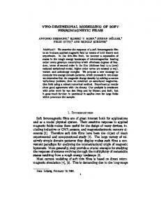
Model selection Two dimensional depth averaged model was generated by using iRIC (international River Interface Corporation) modelling package. Out of the number available solvers within iRIC, such as Nays2D, Morpho2D, FaSTMECH, River2D, SToRM etc., SToRM solver was used in modelling. SToRM stands for System for Transport and River Modeling. This model is a two dimensional flow model using a completely unstructured coordinate system described by a triangular mesh. SToRM is based on concepts of Saint-Venant equation. So that, all the assumptions used in driving the Saint-Venant principle also applicable to the particular model. SToRM uses an unstructured grid, it easily allows very complex channel geometries, including multiple inflows and outflows. The computational methods were chosen to allow treatments of rapidly varied flow, including dam break flows in initially dry channels. Topography and Grid Generation The topographic data used in the model was based on bathymetry data collected from National Building Research Organization of Sri Lanka. From the contour map obtained, a .tpo (topography) file was generated using ArcGIS and incorporated in to the iRIC model. tpo is an ASCII editable file that contains the coordinates and elevation of each data point. The topography data obtained was taken as a triangular irregular network (TIN) and the grid covering the required area of the reservoir was generated. Grid was generated using inbuilt features of the software by inserting a polygon to cover the required area to study (Figure 1).

The 28th International Symposium on Transport Phenomena 22-24 September 2017, Peradeniya, Sri Lanka

Figure 1: Part of the Generated Grid for the Model

Model Calibration For the calibration of the model, measurements of velocities carried out on 17th July 2015 were used. Velocities have been measured at Katugastota in the Mahaweli River, Ambathenna in the Pinga Oya and Polgolla in the Rawan Oya. (Figure 2) Discharges were then calculed using velocity and cross sectional area and the respective discharges were 62.6 m3/s, 0.6 m3/s, 0.1 m3/s from Mahaweli River, Pinga oya and Rawan oya. Discharges from two main tributaries:rawan oya and pinga oya can be considered negligible compared to Mahaweli inflow. The water surface elevation at the barrage gates used as 440.03 m MSL, and no release from gates and discharge was only through the tunnel to power intake.

Figure 3 Comparison of Measured and Calculated Flow Velocities at Katugasthota Railway Bridge for Calibration.

Figure 4 Comparison of Measured and Calculated Flow Velocities for Calibration (Location: Katugasthota Bridge) Model Validation The calibrated model was then validated against field measurement of velocity and depth on 3rd September 2016. Field Measurements Calibration of Current meter A propeller current meter was used for the field measurements. Brand: SAN-EI Serial Number: 85003 Figure 2 Flow velocity measuring locations Using discharge values as upstream boundary condition and water surface elevation as downstream boundary condition, the generated model was simulated for different bed roughness values in terms of Manning coefficient which can be in range of 0.035 to 0.06 for natural streams with boulders and sediment transport. Modelled velocities were compared with measured velocities and best match value, 0.04, was chosen as the bed roughness value. The velocity comparison for bed roughness 0.04 is given in Figure 3 and 4.

The relation between revolutions per second N of the meter and water velocity V in m/s is given by an equation of the form, V=aN+b (10) Current meter was calibrated in the laboratory to obtain the equation V = 0.0453 N – 0.054 (11) Flow Velocity Measurements For calculation of flows and measurement of depths and velocities, three locations were selected. Katugasthota Railway Bridge was chosen for flow measurement in Mahaweli River and validation of the model. Pinga oya discharge was measured at Ambathenna and Rawan oya discharge at Waththegama.

The 28th International Symposium on Transport Phenomena 22-24 September 2017, Peradeniya, Sri Lanka

Water Surface Elevation at the Barrage was observed as 440.78 m (MSL) during flow measuring period. Two gates, gate number 6 and 7 were kept open by 1.2 m which released 64.2 (m3/s). 23.4 (m3/s) discharge was through the power intake tunnel. Validation using field measurement For validation of the model, above field measured conditions were used as boundary conditions and obtained results were acceptable. The velocity comparisons are given in Figure 5

RESULTS AND DISCUSSION The iRIC flow model has been set up for Polgolla reservoir and it can be used to simulate different combinations of inflow and gate opening combinations to identify velocities, water surface elevations and water depths at different locations of the reservoir. With the simulations conducted, velocity patterns for different combinations of inflows and gate openings were identified. Flow Patterns for Different Gate Opening and Inflow Combinations

Velocity (m/s)

0.25

Case 1 2 gates at the right bank are fully open WSE at spill gate = 435.41 m MSL

0.20 0.15 0.10

Total inflow = 55.5 m3/s Water depth at gate landing crest = 1.07 m

0.05 0.00 0

50

Calculated Velocity

100

150 Chainage (m) Measured Velocity

Figure 5 Comparison of Measured and Calculated Flow Velocities at Katugasthota Railway Bridge for Validation

MODEL SIMULATION FOR DIFFERENT GATE OPENING AND INFLOW COMBINATIONS Eight cases of different gate opening combinations and different inflows into the reservoir were identified and simulated using the generated model. Fully open mode of gates were considered to identify flow pattern during reservoir flushing. Number of gates to be kept open for different inflow values were identified using the Elevationdischarge curve for one spillway gate given in Figure 3.10. Inflows at three sections and water surface elevation at the barrage gates were given as boundary conditions. Inflows to the reservoir are specified at upstream of the Mahaweli River, Pinga Oya and Rawan Oya. Inflows were taken proportional to the catchment areas. Outflow was through the barrage gates. Table 1 Different combinations of flow and gate openings considered Case Discharge Gate opening (m3/s) Case 1 55 Two gates at the right bank are fully open Case 2 111 Case 3 55 Two gates at the left bank are fully open Case 4 111 Case 5 277 All 10 gates are fully open Case 6 555 Case 7 137 Five gates at the middle of the spillway are fully open Case 8 277

Figure 6 Velocity pattern for Case 1 Figure 6 depicts that when the right banks gates are opened larger flow velocities are developed at right bank. Lower velocities can be observed closer to barrage gates at left bank during right bank gates openings. When sluicing sediment through right bank gates sediment is expected to deposited closer to gates at left bank. Case 2 2 gates at the right bank are fully open WSE at spill gate = 436.02 m MSL

Total inflow = 111 m3/s Water depth at gate landing crest = 1.68 m

Figure 7 Velocity pattern for Case 2 At a higher inflow of 111 m3/s slightly higher velocities are developed at both banks. But the velocity pattern is similar to that of Case 1. Sedimentation can be expected

The 28th International Symposium on Transport Phenomena 22-24 September 2017, Peradeniya, Sri Lanka

closer to left bank gates and lower velocities in tunnel entrance region could cause sedimentation there as well. Case 3 2 gates at the left bank are fully open WSE at spill gate = 435.41 m MSL

Total inflow = 55.5 m3/s Water depth at gate landing crest = 1.07 m

Figure 10 Velocity pattern for Case 5 Case 6 All 10 gates are fully open WSE at spill gate = 436.02m

Total inflow = 555 m3/s Water depth at gate landing crest = 1.68 m

Figure 8 Velocity pattern for Case 3 When left bank gates are kept open for a discharge of 55.5 m3/s considerable velocity development can be seen closer to the barrage except in extreme right bank. But the velocity at tunnel entrance is very low. Case 4 2 gates at the left bank are fully open WSE at spill gate = 436.02 m MSL

Total inflow = 111 m3/s Water depth at gate landing crest = 1.68 m

Figure 11 Velocity pattern for Case 6 Annual flood of 555 m3/s has been recorded and that flood is simulated in Case 6. High velocities could be seen developed closer to barrage which would cause better sediment sluicing. Case 7 5 gates in the middle are fully open WSE at spill gate = 435.41m

Total inflow = 137.75 m3/s Water depth at gate landing crest = 1.07 m

Figure 9 Velocity pattern for Case 4 The velocity development is almost similar to discharge of 55.5 m3/s in the vicinity of the gates. Considerable velocity can be observed in tunnel entrance as well which shows sediment accumulation would not occur there. Case 5 All 10 gates are fully open WSE at spill gate =435.41 m

Total inflow = 277.5 m3/s Water depth at gate landing crest = 1.07 m 3

For discharge of 277.5 m /s and at all gates kept open, the velocity distribution shows that it would scour whole reservoir bed. Case 5 shows higher velocities would develop at tunnel entrance as well.

Figure 12 Velocity pattern for Case 7 Case 8 5 gates in the middle are fully open WSE at spill gate = 436.02m

Total inflow = 277.5 m3/s Water depth at gate landing crest = 1.68 m

The 28th International Symposium on Transport Phenomena 22-24 September 2017, Peradeniya, Sri Lanka

Figure 13 Velocity pattern for Case 8 Both the Case 7 and Case 8 shows higher velocity developments in the reservoir. Velocities closer to 1 m3/s are shown at tunnel entrance and in other areas of Rawan oya as well. CONCLUSIONS Through results obtained, it can be seen that once gates closer to one bank are opened, pooling occurs at gate closed side and when middle gates are open for higher discharges, higher velocities are developed throughout the reservoir bed. For bed load to move, the bed shear stress should exceed the critical shear stress. The bed shear stress is directly proportional to the velocity gradient and therefore when there are higher velocities, higher bed shear stresses could be expected. Which in turn would be greater than critical shear stress of sediment particles and sluicing would be efficient. From the results of the conducted simulations, it can be concluded that to remove sediment from main reservoir bed in the vicinity of the barrage, opening of middle gates would be a better option than opening of all the gates. Opening of middle gates would develop higher bed shear stresses than opening of all the gates. To remove sediment from Ukuwela tunnel intake region, sluicing would not be the most suitable option. But sluicing while having a discharge greater than 111 m3/s would sluice out considerable amount of sediment from the Tunnel intake region as well. In that case also, opening of five middle gates would generate higher bed shear stresses in the interested area rather than having all the gates opened.

The 28th International Symposium on Transport Phenomena 22-24 September 2017, Peradeniya, Sri Lanka

REFERENCES Herath M. Gunatilake & Chennat Gopalakrishnan (1999) the Economics of Reservoir Sedimentation: A Case Study of Mahaweli Reservoirs in Sri Lanka, International Journal of Water Resources Development, 15:4, 511-526 Jeyakaran T., Ahamed T.F., S.B.Weerakoon, 2015, Two - dimensional flow modelling of Rantembe Reservoir JIA Ya-fei, chan Hsun-Chuan & wang sam s.y, 2009. ‘Three-dimensional numerical modeling of flows in a wide curved channel’, College of Environmental Science and Engineering, Nankai University, Tianjin.pp 78-87 Jonathan M. Nelson, Yasuyuki Shimizu, Hiroshi Takebayashi, Richard R. McDonald, 2010. THE INTERNATIONAL RIVER INTERFACE COOPERATIVE: PUBLIC DOMAIN SOFTWARE FOR RIVER MODELING, 2nd Joint Federal Interagency Conference, Las Vegas, NV, June 27 - July 1, 2010 Morianou G.G., Kourgialas N.N., Karatzas G.P. and Nikolaidis N.P. 2015, 2D simulation of water depth and flow velocity using the mike 21c model, Proceedings of the 14th International Conference on Environmental Science and Technology, Rhodes, Greece, 3-5 September 2015 Neena Isaac, T. I. Eldho & I. D. Gupta (2014) Numerical and physical model studies for hydraulic flushing of sediment from Chamera-II reservoir, Himachal Pradesh, India, ISH Journal of Hydraulic Engineering, 20:1,14-23 Peter W. Downs , Yantao Cui , John K. Wooster , Scott R. Dusterhoff , Derek B.Booth, William E.Dietrich & Leonard S. Sklar (2009) Managing reservoir sediment release in dam removal projects: An approach informed by physical and numerical modelling of non‐ cohesive sediment, International Journal of River Basin Management, pp. 433-452 Rajendra G. Kurup _, David P. Hamilton, Robert L. Phillips 2000, Comparison of two 2-dimensional, laterally averaged hydrodynamic model applications to the Swan River Estuary, Mathematics and Computers in Simulation 51 pp 627–638

S.M. Amiri, N. Talebbeydokhti, & A. Baghlani, 2009, ‘A two-dimensional wellbalanced numerical model for shallow water equations’, Sharif University of Technology. Slobodan P. Simonovic & Sajaad Ahmad, 1999, ‘Comparison of One-Dimensional and Two-Dimensional Hydrodynamic Modeling Approaches for Red River Basin’, Final report to International Joint Commission Ven Te Chow, David R.Maidment & Larry W.Mays, 1988 ‘Applied Hydrology McGrawHil Book Co. Wickramasinghe A., 1995, Mountain forests to mitigate environmental repercussions, proceedings of third international symposium on headwater control, New Delhi, October Yuce, M.I. & Chen, D. 2003. An experimental investigation of pollutant mixing and trapping in shallow costal recirculating flows. In Uijttewaal, W.S.J. & Gerhard, H. J (ed.), Shallow flows; Proc. intern. symp., Netherlands, 16–18 June 2003. Delft: Balkema User’s manual, International River Interface cooperative, 2014