Two-dimensional directional wavelets and the scale-angle ... - CiteSeerX

ZZ ZZ

Two-dimensional directional wavelets and the scale-angle representation J.-P. Antoine 1 and R. Murenzi 2 3 ;

1

Institut de Physique Theorique, Universite Catholique de Louvain B - 1348 Louvain-la-Neuve, Belgium CTSPS, Clark Atlanta University, Atlanta, GA 30314, USA 2

Abstract The two-dimensional continuous wavelet transform (CWT), derived from a square integrable representation of the similitude group of IR2 , is characterized by a rotation parameter, in addition to the usual translations and dilations. This enables it to detect edges and directions in images, provided a directional wavelet is used. First we review the general properties of the 2D CWT and describe several classes of wavelets, including the directional ones. Then we turn to the problem of wavelet calibration. We show, in particular, how the reproducing kernel may be used for de ning and evaluating the scale and angle resolving power of a wavelet. Finally we illustrate the usefulness of the scale-angle representation of the CWT on the problem of disentangling a train of damped plane waves.

UCL{IPT{95{03 May 1995 3

Supported by ONR (Oce of Naval Research), Grant Nr.N0014-93-10561 and by ARPA (Advanced Research Project Agency), Grant Nr.MDA 972-93-1-0013

1. Introduction The wavelet transform (WT) is by now recognized as a fruitful technique in signal and image analysis, which has been applied to a wide variety of physical problems [1]-[3]. We will focus here on the continuous WT (CWT) in two or more dimensions, which is a very ecient and exible tool in image analysis, that is, for the detection and measurement of certain characteristic features in images. By contrast, the discrete or dyadic WT, pioneered by Mallat [4, 5], is often more appropriate for image synthesis, for instance in data compression. Of course, one should always choose the tool that is best adapted to the problem at hand. Thus, given an image, a basic choice must be made right away. For a pointwise analysis, without determination of directions, an isotropic wavelet will suce, such as the radial Mexican hat, but if directional features are to be measured, a directional or oriented wavelet must be used, such as the well-known Morlet wavelet. Our aim here is to study systematically the performances of 2D directional wavelets, both qualitatively and quantitatively, in order to achieve a precise calibration of the wavelet tool. This paper may be seen as a continuation of our previous work [6, 7]. For the convenience of the reader, we will begin by reviewing, in Section 2, the general properties of the 2D CWT, stressing in particular the geometrical aspects. Indeed, a good starting point [8, 9] is to identify the natural operations on an image, namely, translations, rotations ans (global) dilations; these constitute the so-called similitude group SIM(2) of the plane. This group has a natural representation on L (IR ), which is unitary, irreducible and square integrable. Then determines the form of the 2D CWT, exactly as the corresponding representation of the ane group of the line in the 1D case [10]. The structure is exactly parallel, the properties are the same, and so is the interpretation of the CWT as a local lter in all variables. Again, as in 1D, the CWT unfolds the signal, now from 2 to 4 dimensions, and clearly this generates a problem of visualization. A natural solution emerges from a deeper mathematical analysis of the CWT. In physical terminology, the 2D wavelets are nothing but the coherent states associated to the representation of SIM(2). Then, as for most coherent states [11, 12], the parameter space of the CWT, which is SIM(2) itself, may be identi ed with a phase space, namely the coadjoint orbit associated to the representation ; indeed, besides the position variables, the scale-angle pair may be interpreted as spatial frequency variables in polar coordinates. Thus there arise two natural presentations of the CWT, the so-called position and scale-angle representations, respectively, in each of which the second group of variables is kept xed. For further information on the general properties of the 2D CWT, we refer to our previous work [6]. We conclude this survey of the CWT, in Section 3, by a description of various classes of wavelets. In particular, we introduce the directional wavelets, as those whose Fourier 2

2

2

transform is (essentially) supported in a convex cone in spatial frequency space, with apex at the origin. Several examples are exhibited, including the conical or Cauchy wavelet. In the sequel of the paper, we shall concentrate mostly on the scale and angle variables, thus illustrating the usefulness of the scale-angle representation. We begin, in Section 4, by the problem of wavelet calibration: in order to optimize the tool, one has to know quantitatively the performances of the wavelet. This may be achieved in several ways. Particular properties, such as the sensitivity in detecting a discontinuity or selecting a certain direction in an image, may be tested by using adequate benchmark signals. A systematic analysis of this procedure was given in [6], to which we refer for further information. Here we will only illustrate the possibility of ecient directional ltering with a Morlet wavelet on a particularly striking example, which has found a beautiful application in uid dynamics (see Sec. 3.1). More generally, we discuss in detail how the reproducing kernel may be used for calibration. Since it naturally de nes a scale-angle correlation area, it yields a precise de nition the scale and angle resolving power of a wavelet. We show how to evaluate this quantity numerically. The result is then shown to coincide almost exactly, in the case of a Morlet wavelet, with the empirical notion given in [6]. Furthermore, the same notion of resolving power provides a precise lower bound for the discretization grid that is needed for computing numerically the reconstruction formula without information loss { this is in fact nothing but the 2D wavelet equivalent of the familiar Shannon sampling theorem. Finally we conclude the paper by discussing in Section 5 a problem originally stemming from underwater acoustics, namely the measurement of all parameters of a train of damped plane waves. The technique relies upon the successive use of the position and the scale-angle representations of the CWT.

2. The continuous wavelet transform in two dimensions For the sake of completeness we will quickly review in this section the essential features of the continuous wavelet transform in two dimensions, with some emphasis on the geometrical aspects. We refer to [6] and [8, 9] for a detailed discussion (in 2 and in N dimensions, respectively).

2.1 . Images, elementary transformations of the plane and wavelets We will consider two-dimensional signals (images) of nite energy, represented by complexvalued functions de ned on the real plane IR and square integrable, i.e. functions s 2 L (IR ; d ~x): Z ksk = d ~x js(~x)j < 1: (2.1) 2

2

2

2

2

2

2

3

(sometimes it is useful to take s 2 L (IR ; d ~x) \ L (IR ; d ~x) ). In practice, a black and white image will be represented by a bounded non-negative function: 2

1

2

2

2

2

0  s(~x)  M; 8 ~x 2 IR ; M < 1;

(2.2)

2

the discrete values of s(~x) corresponding to the level of gray of each pixel. However it is useful to keep general functions s as above. In fact, one often considers also as admissible signals generalized functions (distributions), such as a delta function (~x ? ~xo ), a plane wave exp(i~k
~x), a fractal measure, etc. The Fourier transform of the signal s is de ned, as usual, by Z 1 ~ sb(k) = 2 d ~k e?i~k:~xs(~x); (2.3) where ~k 2 IR is the spatial frequency and ~k:~x = k x + k x is the Euclidean scalar product. It is useful to write down also the polar coordinate version of the Fourier transform, which involves the eigenvectors fein'; n 2 g of the rotation operators and those of the dilation operators, fri ;  2 IRg, in the same way as the usual Fourier transform involves the (improper) ones of translation operators fe?i~k:~x; ~k 2 IR g: Z 1 dr Z  1 ? in' ?i rf (r; '); ~ f (; n) = 2 d' e r (2.4) r Z 1 1 X rf (r; ') = 21 ein' d ri f~(; n) (2.5) ?1 n ?1 2

2

1

1

2

2

2

2

0

0

=

Of course we recover the well-known fact that the polar coordinate version of the Fourier transform is a combination of a Mellin transform in the radial variable r and a Fourier series in the angle '. All the operations we will apply to a signal s are obtained by combining three elementary transformations of the plane, namely, translations, dilations and rotations. These transformations are represented by the following unitary operators in the space L (IR ; d ~x) of signals: 2

(i) translation : (T ~bs)(~x) = s(~x ? ~b); ~b 2 IR ; (ii) dilation : (Das)(~x) = a1 s( ~xa ); a > 0; (iii) rotation : (R s)(~x) = s(r? (~x));  2 [0; 2); 2

2

2

(2.6) (2.7) (2.8)

where ~b 2 IR is the displacement parameter, a > 0 the dilation parameter,  the rotation angle and the rotation r 2 SO(2) acts on ~x = (x; y) as usual : 2

r (~x) = (x cos  ? y sin ; x sin  + y cos ); 0   < 2: 4

(2.9)

Combining now the three operators, we de ne the unitary operator :

(a; ; ~b) = T ~b DaR ;

(2.10)

which acts on a given function s as : ( (a; ; ~b)s)(~x) = sa;;~b(~x)  a1 s( a1 r? (~x ? ~b));

(2.11)

b a; ; ~b)sb)(~k) = ae?i~b:~k sb(ar? (~k)): ( (

(2.12)

or, equivalently, in the space of Fourier transforms :

If the function s is rotation invariant, we simply omit the index  : ~b (2.13) sa;~b (~x) = a1 s( ~x ? a ): Clearly the three operations of translation, rotation and dilation generate the 2-dimensional Euclidean group with dilations, i.e. the similitude group of IR , here denoted simply G (as usual, the symbol denotes a semidirect product): 2

G  SIM(2) = IR (IR  SO(2)): 2

+

(2.14)

This group is non unimodular, its left and right invariant Haar measure are, respectively: ~b; dr = da d d ~b: d d (2.15) dl = da a a If G is a locally compact group, we recall [11, 12] that a unitary irreducible representation U of G in a Hilbert space H is said to be square integrable, if there exists a nonzero vector  2 H, called admissible, such that the matrix element hU (g)ji is square integrable over the group G (with respect to the left invariant Haar measure). Then we have: 2

2

3

Proposition 2.1 { (i) (:) is a strongly continuous, unitary irreducible representation of

SIM(2) in L2 (IR2; d2~x), and it is the only one, up to unitary equivalence. (ii) The representation (:) is square integrable. A vector 2 L2 (IR2 ) is admissible if the following condition holds:

Z d ~k c  (2) ~ j b(~k)j < 1; jk j 2

2

2

2

where b is the Fourier transform of .

5

(2.16)

The proof of this proposition is straightforward [9]. Irreducibility of means that, for every s 2 L (IR ; d ~x), the linear span of the set 2

2

2

D = fsa;;~b = (a; ; ~b)s; (a; ; ~b) 2 Gg

(2.17)

is dense in L (IR ; d ~x). As for (ii), a straightforward calculation shows that ZZZ da ~ ~ (2.18) a d d b jh (a; ; b) j ij = c k k : Accordingly, a 2D wavelet is de ned as an admissible vector, that is, a complex-valued function 2 L (IR ; d ~x) satisfying the admissibility condition (2.16) which guarantees the square integrability of the representation of G. If is regular enough ( 2 L (IR ; d ~x) \ L (IR ; d ~x) suces), the admissibility condition simply means that the wavelet has zero mean: Z b(~0) = 0 () d ~x (~x) = 0: (2.19) The importance of Proposition 2.1 is twofold. First it puts the CWT on rm mathematical ground { in a way that extends to higher dimensions in a straightforward fashion: the n-dimensional CWT is derived exactly as here from the natural representation of SIM(n) in L (IRn; dn~x). Similarly, the representation generalizes the familiar square integrable representation of the \ax + b" group that lies at the heart of the one-dimensional wavelet transform [10]. Second, it shows that wavelets are nothing but coherent states associated to representation

, that is, elements of the orbit of under the action of G [12]: 2

2

2

2

2

2

3

2

2

2

1

2

2

2

2

2

2

2

~ a;;~b (~x) = [ (a; ; b)](~x);

(a; ; ~b) 2 G;

(2.20)

in the same way as the canonical coherent states associated to the Weyl-Heisenberg group generate the Windowed FT or Gabor transform. Indeed (as for general coherent states), the three unitary operators T ~b; Da; R preserve the admissibility condition, and so does therefore

(a; ; ~b). Hence any function obtained from a wavelet by translation, rotation or dilation is again a wavelet, namely the function a;;~b = (a; ; ~b) , and the orbit is total in the representation space. Furthermore, the identi cation of wavelets with coherent states shows that the CWT is in fact a phase space representation. In classical mechanics, and in particular in the context of geometric quantization [13], it is common to de ne the phase space of a physical system as a coadjoint orbit [14] of the symmetry group of the system. In the present case, an easy calculation [15] shows that SIM(2) has exactly two coadjoint orbits: a two-dimensional orbit of the form f~0g  IR and a four-dimensional orbit of the form IR  IR , where IR  IR n f~0g, corresponding to the unique unitary irreducible 2

2

2

2

2

6

representation (the rst factor corresponds to momentum, the second one to position variables). This orbit is isomorphic to G = SIM(2). Indeed, writing  = a? , the (Haar) measure on G becomes simply the volume element of IR  IR : da d d ~b = d d d ~b = d ~p d ~b; p~  (a? ; ) 2 IR ; ~b 2 IR : (2.21)  a Thus the full 4-dimensional parameter space of the 2D WT, namely G itself, may be interpreted as phase space, with the pair (a? ; )  (; ) playing the role of spatial frequency ~p, expressed in polar coordinates. The same result holds in the 1D case [5, 16]: a? de nes the frequency scale, so that the full parameter space of the 1D WT, the time-scale half plane, is in fact a time-frequency space, thus a phase space. It is amusing to note that the same interpretation is also supported by some physiological evidence, namely the so-called orientation hypercolumns of Hubel and Wiesel [17]-[19]: in certain species, cortical neurons are organized into columns, whose sensibility to position, orientation and frequency variables correspond exactly to the geometry of IR  IR just described. 1

2

2

2

2

2

2

1

2

2

3

1

1

2

2

2.2 . The 2D continuous wavelet transform Let now s 2 L (IR ; d ~x) be an image. Its wavelet transform (with respect to the xed wavelet ), S  W s is, up to normalization, the scalar product of s with the transformed wavelet a;;~b , considered as a function of (a; ; ~b) 2 G : 2

2

2

S (a; ; ~b) = c? = h a;;~bjsi Z ~b = c? = a1 d ~x (r? ( ~x ? a ))s(~x) 1 2

1 2

(2.22)

2

(2.23) R = c? = a d ~k ei~b
~k b(ar? (~k)) sb(~k):(2:24) The relations (2.22)-(2.24) permit to extend the formalism beyond the Hilbert space framework: as explained above, the signal s may be taken as a singular function (a distribution), provided the wavelet is suciently regular (most wavelets used in practice are smooth functions, see below). In the same vein, the wavelet may be required to have a few vanishing moments, as in the 1D case [20, 21]. This condition determines the capacity of the WT to detect singularities. Indeed, if has vanishing moments up to order N , 1 2

2

Z

d ~x xm yn (~x) = 0; 1  m + n  N; 2

(2.25)

then the WT W is blind to polynomials of degree up to N . Equivalently, W detects singularities in the (N + 1)th derivative of the signal [22]. Thus if the signal is rough, a 7

fortiori if it is a measure (as in the analysis of fractals [23]-[25]), it is sucient to take a wavelet with no vanishing moment of order N > 0, i.e. no condition has to be imposed beyond (2.19). The main properties of the CWT are conveniently summarized in terms of the linear map W : s 7! S as follows (proofs may be found in [6, 9]: Proposition 2.2 { De ne the linear map W : L (IR ; d ~x) ! L (G; dg) as [W s](a; ; ~b) = c? = h a;;~b jsi: (2.26) 2

2

2

2

1 2

Then: (1) The map W is a linear isometry from L2 (IR2 ; d2~x) onto a closed subspace H of L2(G; dg): ZZZ da Z 2~ 2 ~ dd b j S ( a; ; b ) j = d2~x js(~x)j2: (2.27) a3 (2) W intertwines between the representation of G in L2 (IR2 ; d2~x) and the left regular representation of G in L2(G; dg):

(W (go)s)(g) = (W s)(go? g); g; go 2 G: 1

(2.28)

In other words, the square integrability of means precisely that belongs to the discrete series. (3) Since it is an isometry, the map W is invertible on its range H , and the inverse transformation is simply the adjoint of W . This means that the image s(~x) may be reconstructed from its wavelet transform S (a; ; ~b) by the formula :

ZZZ da ~ ~ (2.29) a dd b a;;~b(~x) S (a; ; b): If is rotation invariant, the WT S = W s does not depend on  and we obtain a simpler s(~x) = c? =

1 2

2

3

reconstruction formula :

s(~x) = 2 c?1=2

ZZ da ~ a db 2

3

~ a;~b (~x) S (a; b):

(2.30)

(4) The projection from L2 (G; dg) onto the range H of W , the space of wavelet transforms, is an integral operator whose kernel K (a0 ; 0 ; ~b0 ja; ; ~b) is the WT of the wavelet a;;~b itself, that is, K is the autocorrelation function of , also called reproducing kernel:

K (a0 ; 0; ~b0ja; ; ~b) = c? h a ; ;~b j a;;~bi: (2.31) Therefore, a function f 2 L (G; dg) is the wavelet transform of a certain signal i it veri es 1

0

0

0

2

the reproduction property:

f (a0; 0; ~b0) =

ZZZ da ~b K (a0 ; 0; ~b0ja; ; ~b) f (a; ; ~b); dd a 2

3

and H is a reproducing kernel Hilbert space.

8

(2.32)

The statements of Proposition 2.2 hold true for coherent states associated to an arbitrary locally compact group [12]. In the present context of image analysis, they may be rephrased and expanded as follows. (1) The unitarity condition (2.27) means that the family of wavelets f a;;~b; a > 0;  2 [0; 2); ~b 2 IR g generates a resolution of the identity : 1 ZZZ da dd ~b j (2.33) a;;~b i h a;;~b j = I: c a (2) The intertwining property (2.28) means that W is covariant under translations, dilations and rotations [9], which means that the correspondence W : s(~x) 7! S (a; ; ~b) implies the following ones : s(~x ? ~bo ) 7! S (a; ; ~b ? ~bo ) ~ W : a1 s( a~x ) 7! S ( aa ; ; ab ) (2.34) o o o o s(r (~x)) 7! S (a;  ? o ; r? (~b)): 2

2

3

o

o

It is worth noting that, conversely, the wavelet transform is uniquely determined by the three conditions of linearity, covariance and energy conservation, plus some continuity [9]. (3) The formula (2.29) is not only a reconstruction formula, it also means that the the wavelet transform, like its 1-dimensional counterpart, provides a decomposition of the signal in terms of the analyzing wavelets a;;~b , with coecients S (a; ; ~b). Under both interpretations, this formula leads in practice to discretization problems (see Section 2.3). Actually the reconstruction formula (2.29) may be generalized: as in 1D, the wavelet used for the analysis and the one used for the reconstruction need not coincide, they have only to satisfy a cross-admissibility condition [26]. (4) The existence of the reproducing kernel K [27, 28] { shared by the Windowed Fourier transform, and actually by any transform based on a square integrable group representation [12] { is in fact crucial. By its very de nition (2.31), K is a convolution kernel on the underlying group, and as such it enjoys mathematical properties which can be put to practical use. For instance, one may derive useful interpolation properties [10]. Even more interesting, the reproducing kernel yields the most ecient way of estimating the performances of the wavelet tool, as we shall discuss in detail below. Before concluding this section, it is worth recasting the basic formulas (2.22)-(2.24) into dierent forms. (1) In polar coordinates ~x = (r; '), the transform (2.23) reads, with s~b (~x)  s(~x + ~b) : Z 1 dr Z  r r ? = ~ d' a ( a ; ' ? ) r s~b (~x); (2.35) S (a; ; b) = c r 2

1 2

0

0

9

or, in conjugate variables (see (2.5)):

Z1 1 X ? = in ~ d ai e(; n)se~b(; n): e S (a; ; b) = c 1 2

?1

n=?1

(2.36)

(2) As we said above, the CWT is really a phase space realization of the signal. In order to manifest this explicitly, it is convenient to introduce the following notation. For any vector ~x = (x; y)  (r; '), de ne the matrix

0 1 x ? y A = r r' : (~x) = @ y x

(2.37)

Then (~x)~z = (~z)~x and r (~x) = (~x)~e , where ~e denotes a unit vector in the direction . Introduce now the phase space vectors (in polar coordinates) (2.38) ~p = (a? ; ); ~v = (a; ?)  kp~I~pk ; where I denotes the re ection with respect to the x-axis. Clearly (p~)(~v) = I: The variable p~ is more natural, in view of the phase space analysis described in Section 2.1. It follows also the common practice in image processing: a = 0 is the horizon in spatial frequency plots, corresponding to extremely high frequencies. On the other hand, using the variable ~v sometimes simpli es the computations (see Section 5, for instance). We come back now to the expression (2.24) of the CWT. One has immediately 1

2

ar? (~k) = (~v)~k = (~k)~v = (p~)? ~k = (~k) kp~I~pk ;

(2.39)

1

2

and therefore the CWT may be written explicitly in terms of phase space variables (~v; ~b) or (p~; ~b):

Z ? = ~ ~  S (a; ; b)  S (~v; b) = c k~v k d ~k ei~b
~k b((~v)~k) sb(~k) Z  S~(p~; ~b) = c? = kp~ k? d ~k ei~b
~k b((p~)? ~k) sb(~k) 1 2

1 2

2

1

2

1

(2.40) (2.41)

2.3 . Understanding the CWT As in 1D, we will assume that the wavelet is fairly well localized both in position space (~x) and in spatial frequency space (~k). Then so does the transformed wavelet a;;~b, with eective support suitably translated by ~b, rotated by  and dilated by a. Because (2.23) is a convolution with a function of zero mean, the transform S (a; ; ~b) is appreciable only in 10

those regions of parameter space (a; ; ~b) where the signal is: we get an appreciable value of S only where the wavelet a;;~b \matches" the features of the signal s. In other words, the CWT acts on a signal as a local lter in all 4 variables a; ; ~b : S (a; ; ~b) `sees' only that portion of the signal that `lives' around a; ; ~b and lters out the rest. Let us make more precise the support properties of . Assume and b to be as well localized as possible (compatible with the Fourier uncertainty principle), that is, has for essential support (i.e. the region outside of which the function is numerically negligible) a `disk' of diameter T , centered around 0, while b has for essential support a `disk' of diameter , centered around ko. Then, for the transformed wavelets a;;b and ba;;b we have, respectively: . ess supp a;;b is a `disk' of diameter ' aT around b, rotated by r ; . ess supp ba;;b is a `disk' of diameter ' =a around ko=a, rotated by r ;. Notice that the product of the two diameters is constant (we know it has to be bounded below by a xed constant, by Fourier's theorem). Thus the wavelet analysis operates at constant relative bandwidth,
k=k = const, where k  j~kj (in other words, it is a constantQ analysis). Therefore, the analysis is most ecient at high frequencies or small scales, and so it is particularly apt at detecting discontinuities in images, either point singularities (contours, corners) or directional features (edges, segments). All together, as in the 1D case, the 2D wavelet transform may be interpreted as a mathematical, direction selective, microscope, with optics , magni cation 1=a and orientation tuning parameter . Two features must be emphasized here: the magni cation 1=a is global, independently of the direction, and there is the additional property of directivity, given by the rotation angle . The reproduction property (2.32) means that the information contained in the WT S (a; ; ~b) is highly redundant. This redundancy may be eliminated (this is the basic idea behind the discrete WT), or exploited, either under the form of interpolation formulas or for discretizing the reconstruction formula (2.29), as needed for numerical evaluation, without loss of information. The integral is replaced by a sum over a discrete (but in nite) family of wavelets a ; ;~b , which can be chosen in such a way that the formula remains exact: j

k

l

s(~x) '

X jkl

aj ;k ;~bl

S (aj ; k ; ~bl ):

(2.42)

The existence of such a family, called a frame, may be proven along the same lines as in the 1D case [16, 29], with similar results [8, 9]. Thus the 2D wavelet transform too obeys a sampling theorem resembling the standard Shannon theorem of signal analysis, only more complicated. In practical applications, the in nite sum will be truncated (a few terms will often suce) and the approximate reconstruction so obtained is numerically stable [16]. The problem, of 11

course, is how to choose the sampling grid in an optimal fashion. There are theorems that give lower bounds on the density of sampling points, but this is of little help in practice. For the (a; ) variables, in particular, the sampling points are quite often xed empirically in the literature, for instance on the basis of biological considerations or symmetry requirements [4, 5, 22, 30, 31] (for instance, the hexagonal symmetry seems to have a preferred role in vision problems). Now the CWT described here oers the possibility of an intrinsic, quantitative, solution of this sampling problem, by exploiting the properties of the reproducing kernel K , as we shall see in Sec. 4.2 below.

2.4 . Implementation: the two basic representations

The rst problem one faces in practice is that of visualization of the CWT. Indeed S (a; ; ~b) is a function of 4 variables: 2 position variables ~b 2 IR , and the pair (a; ) 2 IR  [0; 2) ' IR . One may say that the CWT W has unfolded the signal from 2 to 4 dimensions. This feature explains its eciency in decoupling singularities, but at the same time makes the data much heavier. As a consequence, some of the variables must be xed for visualization of the CWT. There are many possibilities, but the interpretation of the parameter space as phase space given above suggests two natural ways of presenting the CWT, using 2-dimensional sections of the parameter space: 2

+

2

(i) the position representation, where a and  are xed and the CWT is considered as a function of position ~b alone (this amounts to take a set of snapshots, one for each value of (a; ), which may then be collected together into a movie). (ii) the scale-angle representation: for xed ~b, the CWT is considered as a function of scale and angle (a; ), i.e. of spatial frequency; in other words, one looks at the full CWT through a keyhole located at ~b, and observes all scales and all directions at once. The position representation is the standard one, and it is useful for the general purposes of image processing: detection of position, shape and contours of objects; pattern recognition; image ltering by resynthesis after elimination of unwanted features (for instance, noise). The scale-angle representation will be particularly interesting whenever scaling behavior (as in fractals) or angular selection is important, in particular when directional wavelets are used. In fact, both representations are needed for a full understanding of the properties of the CWT in all 4 variables, and the reproducing kernel K should be studied in both (see also the discussion at the end of Section 3.4 below). For the numerical evaluation, discretization of the WT in either representation and systematic use of the FFT algorithm, will lead to a numerical complexity of 3N N log(N N ), 1

12

2

1

2

where N ; N denote the number of sampling points in denotes the number of sampling points in the variables (bx; by ) or (a; ). We refer to [6] for a more detailed discussion. Whichever representation we use, we end up with a function of two variables, either in Cartesian coordinates ~b, or in polar coordinates (a; ): In both cases, the function may be real or complex (see the examples below). In the latter case, it will be often represented through its modulus and phase. It turns out that the phase is particularly instructive, as was already the case in 1D [6]. 1

2

3. Choosing an adequate analyzing wavelet 3.1 . Universal wavelets The next step in the analysis is to choose an analyzing wavelet . There are two possibilities. Either one chooses a standard, `universal', wavelet, or one turns to a dedicated one, better adapted to the problem at hand. for the rst type, the most popular wavelets are familiar from the 1D case. 3.1.1. The 2D Mexican hat or Marr wavelet In its isotropic version, this is simply the Laplacian of a Gaussian: 1 (3.1) H (~x) = (2 ? j~xj ) exp(? j~xj ): 2 This is a real, rotation invariant wavelet, with two vanishing moments, of order 0 and 1. There exists also an anisotropic version, but it is of little use in practice, because it still acts as a second order operator and detects singularities in all directions. Indeed it is not a directional wavelet, in the technical sense de ned below. Hence the Mexican hat will be ecient for a ne pointwise analysis, but not for detecting directions. Closely related are the iterated Laplacians of the Gaussian: 1 m (3.2) mH (~x) = (?
) exp(? j~xj ); m = 1; 2; : : : : 2 These wavelets behave very much like the usual Mexican hat (m = 1), only they have more vanishing moments, hence they are more sensitive to discontinuities. 2

2

2

3.1.2. The 2D Morlet wavelet This is the prototype of an oriented wavelet: Mor

(~x) = exp(i~ko
~x) exp(? 21 jA~xj ) + corr. term: 2

13

(3.3)

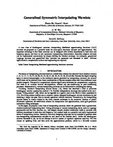
The parameter ~ko is the wave vector, and A = diag[? = ; 1];   1; is a 2  2 anisotropy matrix. The correction term enforces the admissibility condition b (~0) = 0, but it is numerically negligible for j~koj  5:6 and will usually be dropped. In that case, putting  = 1, we obtain the function: 1 (3.4) G (~x) = exp(i~ko
~x) exp(? j~xj ); 2 well-known in the image processing literature under the name of Gabor function [30]. The modulus of the wavelet G is a Gaussian, whereas its phase is constant along the direction orthogonal to ~ko. Thus the wavelet G smoothes the signal in all directions, but detects the sharp transitions in the direction perpendicular to ~ko. The angular selectivity increases with j~koj, and even more so if, in addition, one introduces some anisotropy by taking  > 1. Then the modulus becomes a Gaussian elongated in the x direction, i.e. its `footprint' is an ellipse p with large axis on the x-axis and ratio of axes equal to . Clearly this wavelet will detect preferentially singularities (edges) in the x direction, and its eciency increases with . The best selectivity will be obtained by combining the two eects, i.e. by taking ~ko perpendicular to the large axis of the ellipse, thus ~ko = (0; ko). The resulting complex wavelet, denoted M , is the one we shall use in the sequel: ! x 1 ik y (3.5) exp ? 2 (  + y ) : M (x; y ) = e It is shown in Figure 1, for ko = 5:6 and  = 1: 1 2

Mor

2

2

o

2

3.2 . Dierence wavelets Many other wavelets (or lters) have been proposed in the literature, often designed for a speci c problem. An interesting class consists of wavelets obtained as the dierence of two positive functions, for instance a single function h and a contracted version of the latter. If h is a smooth non-negative function, integrable and square integrable, with all moments of order one vanishing at the origin, then the function given by the relation : (3.6) (~x) = 1 h( ~x ) ? h(~x) (0 <  < 1) is easily seen to be a wavelet satisfying the admissibility condition (2.19). Since h is typically a smoothing function, the wavelet is called the `Dierence-of-Smoothings' or DOS wavelet [19]. Notice that h, and thus also , need not be isotropic. Several particular cases have been used in the literature. 2

3.2.1. The DOG wavelet Taking for h a Gaussian, one obtains the DOG or Dierence-of-Gaussians lter: 1 e?j~xj2 = 2 ? e?j~xj2 = ; (0 <  < 1): D (~x) =  2

2

2

14

(3.7)

The DOG lter is a good substitute for the Mexican hat (for ? = 1:6, their shapes are extremely similar), frequently used in psychophysics works [18, 19, 32]. It was also considered by Grossmann [33] for signal analysis, together with more general linear combinations of Gaussians. 1

3.2.2. The DOM lter The DOM or Dierence-of-Mesas lter, corresponding to a function h which is a smoothed version of the characteristic function of a disk (a `mesa' function) [34]. 3.2.3. The optical wavelet Another interesting dierence lter is simply a sharp band-limited annular lter (thus, the dierence of two concentric disks in spatial frequency space):

bB (~k) = 1; for K  j~kj  K ; = 0; otherwise 1

2

(3.8)

Thus the DOM lter is the position space equivalent of the present one, but in a smoothed version. This lter is used systematically by Arneodo et al. [24, 35] for the so-called optical WT, which consists in a hardware (optical) realization of the lter. 3.2.4. Object adapted dierence wavelets More generally, the concept of dierence wavelet is useful for reducing noise in images. Take an image, consisting of an object to be identi ed, embedded in noise or clutter. Let h(~x) be an averaged version of the image. Then the corresponding dierence function (~x) given by (3.6) is a wavelet ideally suited for the analysis of the object in question. Indeed the dierence operation substantially reduces the background noise, and incorporates a maximal amount of resemblance with the object (a priori information). This subtraction technique is commonly used in the treatment of astrophysical images for enhancing the relevant information (galaxies, e.g.), while reducing the noise (the brilliant background sky).

3.3 . Directional wavelets Edge detection is a classical problem in image processing, for which many techniques have been developed [36]-[40]. In the present context, if one wants to detect oriented features (segments, edges, vector eld,. . . ), one needs a wavelet which is directionally selective. To be precise, we will say that a given wavelet is directional if the eective support of its Fourier transform b is contained in a convex cone in spatial frequency space f~kg, with apex 15

at the origin, or a nite union of disjoint such cones (in that case, one will usually call multidirectional). According to this de nition, the anisotropic Mexican hat is not directional, since the support of bH is centered at the origin, no matter how big its anisotropy is, as can be seen on Figure 2(a); and, indeed, detailed tests con rm its poor performances in selecting directions [6]. As examples of directional wavelets, we will describe brie y the Morlet wavelet (and its multidirectional relatives) and the conical or wavelets. Note that other wavelets, although not directional in the sense of the above de nition, may have some capabilities of directional ltering. Such are, for instance, the gradient wavelets @x exp(?j~xj ) or @x@y exp(?j~xj ). The latter, in particular, looks promising for the detection of corners in a contour [37, 39]. 2

2

3.3.1. The Morlet wavelet >From (3.5), we get:

  bM (~k) = det A? exp ? 1 jA? (~k ? ~ko)j   1 2 p =  exp ? 2 [kx + (ky ? ko) ] : 1

1

2

2

2

(3.9)

The function bM , with  = 5 and rotated by  = 45o, is shown (in level curves) in Figure 2(b); its eective support is centered at ~ko and is contained in a convex cone, that becomes narrower as  increases: this is indeed the archetype of a directional wavelet. 3.3.2. Multidirectional or `fan' wavelets Given a directional wavelet as above, it is easy to build a multidirectional one, with n-fold symmetry, simply by superposing n suitably rotated copies of : ? 1 nX ( ~ x ) = (r? (~x)); k = k 2 ; k = 0; 1; : : : n ? 1: n n k n 1

k

(3.10)

=0

Taking, for instance, n = 4 and for a Morlet wavelet, we get the following real wavelet with 4-fold symmetry, shown in Figure 3: 1 ? 1 x2 y2 : (3.11) M (x; y ) = (cos ko x + cos ko y ) e 2 2 This wavelet lters out all features which are not primarily horizontal or vertical. In the same way, one gets wavelets with symmetry 6 or 10, which may nd applications, respectively, in biological problems or the analysis of quasi-crystals. In general, multidimensional wavelets should be useful for pattern recognition. (

4

16

+

)

Notice that a similar construction was proposed by Watson [34]. His fan lters result from a further restriction of the DOM lter, obtained by repeated bisection of the frequency space: the allowed directions  are thus restricted to a fan-shaped region : 0  2  2n? (n = 2; 3; : : :): (3.12) 2 This construction may then be generalized to arbitrary angles [41]. 1

3.3.3. Conical or Cauchy wavelets In order to achieve a genuinely oriented wavelet, it suces to consider a smooth function bS (~k) with support in a strictly convex cone S in spatial frequency space and behaving inside S as P (kx; ky )e?~
~k , with ~ 2 S , or P (kx; ky )e?jkj2 , where P (:) denotes a polynomial in two variables. Let us study in some detail the former case. Let C  C (; ) be the convex cone determined by the unit vectors ~e;~e , where  < ; ?  <  and ~e  (cos ; sin ): The axis of the cone is ~ = ~e 21  : Then one has: ( + )

f~k 2 IR :   arg(~k)  g f~k 2 IR : ~k
~  ~e
~ = ~e
~ > 0g:

C (; ) = =

2

(3.13)

2

The dual cone, also convex, is ~ ~) = f~k 2 IR ; ~k
~k0 > 0; 8 ~k0 2 C (; )g; Ce  C ( ; 2

(3.14)

where ~ =  + =2; ~ = ? =2, and therefore ~e
~e = ~e
~e = 0. Thus the axis of Ce is ~ again. In these notations, we may de ne a 2D Cauchy wavelet, with support in C = C (; ), for any ~ 2 Ce and l; m 2 , as: ~

~

8

blmC ) (~k) = < : (

(~k
~e )m (~k
~e )l e?~k
~ ; ~k 2 C (; ) 0; otherwise: ~

~

(3.15)

An explicit calculation, given in Appendix A, then yields the following result: (C ) ?l?1 lm (~x) = const. (~z
~e )

(~z
~e )?m? ; 1

e where we have introduced the complex variable ~z = ~x + i~ 2 IR + iC: For instance, taking  = 0; = =2; ~ = ~ and l = m = 1; one gets: C (~x) = 1 (1 ? ix)? (1 ? iy )? ; 2

(3.16)

2

( ) 11

2

17

2

(3.17)

i.e. the product of two 1D Cauchy wavelets [45], that is, derivatives of the Cauchy kernel (z ? t)? ) | hence the name. We show in Figure 4 the wavelet b C (~k) for C = C (?10o; 10o); this is manifestly a highly directional lter. Notice that, since the function blmC (~k) has support in the convex cone C = C (; ) and is of fast decrease at in nity, it follows from general theorems [42] that its Fourier transform C C e lm (~x) is the boundary value of a function lm (~z), holomorphic in the tube IR + iC: In that sense, the Cauchy wavelets yield a genuine multidimensional generalization of the 1D Hardy functions obtained as Fourier transforms of progressive wavelets [43], much more so than the so-called 2D Hardy functions de ned by Dallard and Spedding [44], which seem to us a rather ad hoc construction. ( ) 44

1

(

(

)

)

(

)

2

3.4 . Directionless wavelets At the other extreme, it is sometimes useful to have a fully rotation invariant wavelet. Typical examples are the isotropic Mexican hat, which reads in frequency space:   bH (~k) = j~kj exp ? 1 j~kj ; (3.18) 2 or the isotropic versions of the dierence wavelets described in Section 3.2 (DOG, DOM, optical). Another one is the Halo wavelet introduced in [44]:   b (~k) = exp ? 1 (j~kj ? j~koj ) : (3.19) 2 Of course, this function can be taken as a wavelet only if j~koj is large enough; otherwise a correction term is needed, as usual (in fact it is easy to design a genuine wavelet with a similar behavior). Such ring-shaped wavelets could be adequate for detecting the presence of rings in an image. A striking example is the detection of gravitational arcs or arclets in the images of galaxy clusters { a precious source of cosmological information! We emphasize, however, that, even if no preferred direction is relevant or known, there is no need to use a directionless wavelet as above. Indeed, the scale-angle representation permits precisely to control all directions at the same time. Even more, the directional selectivity of the wavelet may be exploited to increase the resolving power, as illustrated in the example of the wave train discussed in Section 5. 2

2

2

Halo

2

4. Evaluation of the performances of the CWT Given a wavelet, what is the resolving power of the associated wavelet microscope, in particular what is its angular and scale selectivity ? What is the minimal discretization grid for the 18

reconstruction formula (2.29) that guarantees that no information is lost ? The answer to both questions resides in a quantitative knowledge of the properties of the wavelet at hand, that is, the tool must be calibrated. To that eect, one takes the WT of particular, standard signals. Three such tests have proven useful, and in each case the outcome may be viewed either at xed (a; ) (position representation) or at xed ~b (scale-angle representation).

 Point signal: for a snapshot at the wavelet itself, one takes as signal a delta function, i.e. one evaluates the impulse response of the lter: h a;;~bji = a1 ( a1 r? (?~b)):

(4.1)

This yields the eective support of , in each pair of variables ~b or (a; ).

 Reproducing kernel: taking as signal the wavelet itself (here normalized to c = 1), one obtains the reproducing kernel K , which measures the correlation length in each variable a; ; ~b : Z 1 ~ ~ (4.2) K (a; ; bj1; 0; 0) = h a;;~bj i = a d ~x ( a1 r? (~x ? ~b)) (~x): As we shall see below, a detailed analysis of K yields a de nition of the resolving power of the wavelet in each variable, and the result ts perfectly with the empirical de nitions given previously [6]. 2

 Benchmark signals: for testing particular properties of the wavelet, such as its ability to detect a discontinuity or its angular selectivity in detecting a particular direction, one may use appropriate `benchmark' signals.

4.1 . Calibration of a wavelet with benchmark signals As with any tool, calibration of a wavelet with respect to a given process requires the use of benchmark signals. A systematic analysis was presented in [6], for the following operations: - detection of a line singularity (rod) - detection of a given direction (semi-in nite rod, several segments with dierent orientations) - measurement of the opening angle of a wedge. In all cases, the response of the CWT was given as a function of the various parameters of the wavelet used, e.g. wave number ko, anisotropy  and misorientation, in the case of a Morlet wavelet. 19

p

A general conclusion was that, for a suciently large value of the product ko , the Morlet wavelet is able to detect the orientation of a segment with a high selectivity, of the order of a few degrees. Thus it is ecient also for directional ltering. In order to illustrate the point, we analyze in Figure 5 a pattern made of a large number of rods in dierent directions (a). An application of the CWT with a xed direction, here horizontal, selects all the rods which have roughly the same direction (b), whereas the other ones, which are misaligned, yield only a faint signal corresponding to their tips, in agreement with the behavior discussed in [6]. Since this is in fact noise, one performs a thresholding to remove it, thus getting a clear picture (c). The same two operations are then repeated with various successive orientations of the wavelet. In this way, one can count the number of objects that lie in any particular direction. As a matter of fact, the CWT (and the discrete WT as well) has been applied to several problems in uid mechanics, especially in the analysis of 2D developed turbulence (e.g. for the detection of coherent structures), see [46] for a review. But almost all works deal with pointwise analysis, with an isotropic wavelet, such as a Mexican hat or an iterated laplacian of a Gaussian (the values m = 4; 8; 16 are used, the interest being their large number of vanishing moments). A remarkable exception is a beautiful application of directional ltering to a problem of uid dynamics, namely the visualization and measurement of the velocity eld of a 2D turbulent ow around an obstacle [47, 48], following exactly the procedure described above. Velocity vectors are materialized by small segments. Then the WT with a Morlet wavelet is computed twice: rst the WT selects those vectors that are closely aligned with the wavelet; then the analysis is repeated with a wavelet oriented in the orthogonal direction, thus completely misoriented with respect to the selected vectors (0 ' 90o): now the WT sees only the tips of the vectors and their length may be easily measured. Using appropriate thresholdings, the complete velocity eld may thus be obtained, in a totally automated fashion, with an eciency sensibly better than with more traditional methods.

4.2 . Scale-angle correlation area and resolving power of the wavelet 4.2.1. Scale and angle resolving powers: de nition The best way of testing the correlation length of the wavelet is to analyze systematically its reproducing kernel. First one can plot K itself in the scale-angle representation, that is, in polar coordinates (a; ). The example of the Morlet wavelet has been given in [6], for several values of (ko and ). As expected, the eective support of K gets more peaked as ko and/or  increases. On such a plot, one can read o directly the angular width
 = max ? min of K and its scale range
a = amax =amin , where [amin; amax ] is the eective support of K in 20

the variable a. Let now the wavelet have its eective support in spatial frequency in a cone of aperture
' = ' ? ' , between scales  and  , as shown in Figure 6: 2

1

1

2

'  '  ' and      : 1

2

1

(4.3)

2

Then, going over to spatial frequency space, in polar coordinates ~k = (; '), one gets: Z b b ~ ~ K  K (a; ; bj1; 0; 0) = h a;;~bj i = a d ~k ei~k
~b b(a; ' ? ) b(; '): 2

(4.4) Then the support properties (4.3) of b imply that K is nonvanishing i   a   and '  ' ?   ' , so that the eective support of the reproducing kernel K is given by amin =  =  a  amax =  = for the scale variable and min = ?
'    max =
' for the angular variable. The corresponding domain in the (a; ) plane is the scale-angle correlation area of the wavelet. Its area is given by 1

2

1

2

1

h

2

2

i

h

i

1

AK = ( = ) ? ( = )
' = amax ? amin
': 2

1

2

1

2

2

2

2

(4.5)

It follows that we may de ne the wavelet parameters (or resolving power) in terms of those of K as: . scale width or scale resolving power (SRP):

q

p


 =  = =
a = amax =amin; 2

1

. angular width or angular resolving power (ARP):
' = 1
 = 1 (max ? min ): 2 2 In the same way, the scale-angle correlation area AK is related to the area A b of the eective support of the wavelet b by the relation ! 1 1 AK = 2  +  A b: (4.6) 2 2

2 1

4.2.2. Scale and angle resolving powers: numerical evaluation Given the directional wavelet , we may characterize its eective support in spatial frequency space exactly as in 1D [49]. We say that b is located at ~ko if Z ~ko = d ~k ~kj b(~k)j : (4.7) 2

21

2

Similarly, its width in the direction ~ is given by 2w~, where:

= Z 1 b ~ ~ ~ ~ ~ d k j(k ? ko)
 )j j (k)j : w~ = b 2

k k

2

2

1 2

(4.8)

Typically one may suppose that (after a suitable rotation) the supporting cone of b is vertical, i.e. ~ko = (0; ko). Then the width of b in the horizontal and vertical directions are given by 2wx; 2wy , respectively, where (see Figure 7): 1 Z d ~k k j b(~k)j  = x b

wx =

k k

2

k k

2

2

2

1 2

1 Z d ~k (k ? k ) j b(~k)j  = : y o b

wy =

2

2

1 2

(4.9)

Then the wavelet is concentrated in the ellipse

! ! kx + ky ? ko = 1: (4.10) wx wy Taking intercepts with the ky -axis, we obtain for the radial support of b:  = ko ? wy ;  = ko + wy ; and thus the scale resolving power is + wy : (4.11) SRP ( ) = kko ? o wy As for the angular resolving power ARP, we consider the tangents ky = qkx to that ellipse, with q = cot . Then a straightforward calculation yields: 2

2

1

2

ARP ( ) = 2 cot? qq k ?w = 2 cot? o y : w 1

2

2

1

x

(4.12)

In particular, for ko >> wy , we get:

ARP ( ) = 2 cot? wko : x For instance, if is the (truncated) Morlet wavelet (3.5), one obtains: wx = p1 ; wy = p1 ; 2 2 1

22

(4.13)

(4.14)

and therefore:

p

SRP ( M ) = kop2 + 1 ko 2 ?q1 ARP ( M ) = 2 cot? (ko ? 1); 1

2

and, for ko >> 1:

(4.15)

p

(4.16) ARP ( M ) = 2 cot? (ko ): This last expression coincides with the empirical result of [6]: the angular sensitivity of M p depends only on the product ko . Notice also that the SRP is independent of the anisotropy factor . We conclude with two remarks. First, the widths wx; wy characterize completely the wavelet. For instance, for a given numerical precision , the bandwidths in kx; ky may be expressed in terms of wx; wy and , and thus also the bound on the sampling frequency imposed by Shannon's theorem. These numerical aspects will be discussed elsewhere.. Second, the notion of angular resolving power oers also the possibility of testing quantitatively the eect of the correction term in the full Morlet wavelet (3.3). We have plotted in Figure 8 the ARP (in degrees) as a function of j~koj. This graph shows that the correction term, although negligible for j~koj  6, still improves the ARP by 1 or 2 degrees (notice that all calibration curves given in our previous work [6] were estimated with the correction term). 1

4.2.3. Application to sampling in the scale-angle plane Suppose we have a signal s which ranges in spatial frequency between m and M and we want to analyze it with the wavelet just discussed. Then the extreme scales that are needed are, respectively, am = m = and aM = M = , where  ;  are the wavelet parameters. Thus the scale range will be: aM = M =m =
 : (4.17) am  =
 Therefore, if the discretization is performed on a dyadic scale, the signal s will be completely analyzed by the family of wavelets (` lter bank') f ba ; (~k)g; where aj = m
2j ; j = 0; 1; : : : ; M ? 1; ` =
'
`; ` = 0; 1; : : : ; L ? 1; 1

2

1

2

signal

2

1

wavelet

j

`

1

with

M = integer part of log



signal

2

wavelet

23

!

; L = integer part of
2' :

(4.18)

The resulting scheme is illustrated in Figure 9 (similar discussions, albeit mostly qualitative, were given in [22] and [34]). It is gratifying that these analytical estimations t very well with the empirical parameters determined previously [6]. We emphasize that such an analysis is only possible within the scale-angle representation. Thus it requires the use of the CWT, and it is completely outside of the scope of the discrete WT, which is essentially limited to a Cartesian geometry (orthogonal wavelet bases are not available in polar coordinates).

5. Application: disentangling of a plane wave train The basic problem is to decompose a complex signal into single components which have a simple form, more or less known a priori, and to isolate their individual contribution to the WT; this is the key for noise ltering or elimination of unwanted components. A typical example in 1D is the estimation of spectral lines (e.g. NMR spectroscopy, geophysical time series). The problem is to identify with great precision the position of the peaks (local maxima) and to measure their parameters [50]. Another 1D example is the analysis of refracted waves in underwater acoustics [51], although this particular example is in fact a 3D situation. We shall consider here the 2D version of the problem [52]. The signal is a superposition of plane waves, damped in a given direction, and we want to measure the various parameters of each component. We shall take the signal in the following form : N X (5.1) f (~x) = cn ei~k
~x e?~l
~x; n

n

n=1

where cn = Anei , with An and n respectively the modulus and phase of the nth component at the origin; ~kn is the wave vector and the vector ~ln in a (oriented) damping factor. In terms of the complex vector ~zn = ~kn + i~ln, the signal and its Fourier transform read, respectively (here  is a complex delta function): n

f (~x) =

N X n=1

X cn ei~z
~x; fb(~k) = cn (~k ? ~zn ) N

n

n=1

(5.2)

The choice of an exponential damping factor exp(?~ln
~x) makes of course the computation especially simple, but it is by no means essential. For instance, similar results would be obtained with a damping factor acting in one direction only, such as #(~ln
~x) exp(?~ln
~x), where # is the jump function or a smoothed version thereof. The important point is that the perturbation be local: the method still allows the determination of the various parameters suciently far away from the perturbation (as in 1D). 24

Let now be a wavelet, normalized to c = 1: Then a straightforward evaluation yields the WT of the signal (5.1):

X F (a; ; ~b) = a cn ei~z
~b b(ar? (~zn )): N

(5.3)

n

n=1

Of course, the linearity of the WT implies that the result is the linear superposition of the contributions of the various components. Going over to the phase space notation introduced in Section 2.2, (5.3) becomes

X F (a; ; ~b)  F (~v; ~b) = k~vk cn ei~z
~b b((~zn ) ~v) N

n=1 N X

 F~ (p~; ~b) = kp~k?

1

n=1

(5.4)

n

cn ei~z
~b b((p~)? ~zn)

(5.5)

1

n

This expression shows explicitly that the WT F (a; ; ~b) is a function of the phase space variables ~v; ~b, or ~p; ~b. To get numerically precise results, we take as analyzing wavelet a Morlet wavelet of parameters ko; , as given in (3.5) or (3.9). We denote by ~kn = kn~e , resp. ~ln = ln~e , the parameters of the incoming wave. It is then straightforward to evaluate explicitly the expression (5.4). In a rst step, we x ~b and analyze the ~v  (a; ) dependence of F (~v; ~b). Writing n

n

X F (~v; ~b) = k~vk c~b;n Fn(~v); N

(5.6)

n=1

we observe that, for each n, the modulus jFn(~v)j has a unique maximum localized at ~vnmax  max (amax n ; ?n ), where

h

i

(vnmax)x = D? kokn kn sin n ? ln( sin n cos(n ? n) + cos n sin(n ? n)) ; h i (vnmax )y = D? kokn kn cos n ? ln( cos n cos(n ? n) ? sin n sin(n ? n)) ; 1

1

2

2

2

2

with

D = (kn + ln) ? knln[( + 1) sin (n ? n) + 2 cos (n ? n)]: Similar expressions may be written for N X ? ~ ~ c~b;n F~n(p~); F (p~; b) = kp~k 4

4

2 2

2

2

2

1

n=1

? max where each jF~n(p~)j has a unique maximum at p~nmax  ((amax n ) ; n ). We evaluate these expressions in two simpler cases. 1

25

(1) A Morlet wavelet with isotropic modulus, i.e.  = 1: Then we obtain: (vnmax)x = kko?knl sin n; (vnmax )y = kko?knl cos n; 2

that is,

n

2

2

n

n

 kokn max k~vnmax k = amax n = jk ? l j ; n = n ? 2 sign (kn ? ln ); 2

2

and

(5.7)

2

n

n

2

n

2

(5.8)

jFn(~vnmax )j = exp 21 ko ln (kn ? ln)? :

(5.9) Thus increasing the wave vector ko enhances all the local maxima, provided ln 6= 0. 2 2

2

2

1

(2) A pure plane wave, i.e. ln = 0; 8 n: Now we get (vnmax )x = kko sin n; (vnmax )y = kko cos n: (5.10) n n and ko max  max k~vnmax k = amax (5.11) n = k ; n = n ? 2 ; jFn (~vn )j = 1: n Thus, in this case, the position and amplitude of the local maxima do not depend on the anisotropy . Now, in the full transform (5.3), each term has its own local maximum, but these need not be well separated : one maximum may hide another one, totally or partially. This masking eect will happen, for instance, when:  one component has a much bigger amplitude, jc~b;nj >> jc~b;mj, for all m not equal to n (total masking);  two wave vectors are close to each other, ~kn ' ~km, but with dierent amplitudes, jc~b;nj > jc~b;mj (partial masking). In both cases, the two waves can be separated, by increasing the selectivity of the wavelet (for instance, using a Morlet wavelet with a more anisotropic modulus). If the two waves have close wave vectors (~kn ' ~km) with similar amplitudes (jc~b;nj ' jc~b;mj), but dierent damping vectors (~kn 6= ~km), then they can still be separated, by changing the observation point ~b. Otherwise the method will fail, the two waves interfere inextricably, none of them dominates the other one. When the masking eect is not too important, the maxima will be suciently prominent that the interferences between the dierent components will become negligible (in the modulus) and one may write

X jF (~v; ~b)j ' k~vk jc~b;nj jFn(~v)j; N

n=1

26

(5.12)

This is the formula used in practice (see the example below). Now we come back to the full transform (5.3) and evaluate it successively at every local max maximum ~vnmax  (amax n ; ?n ), thus reverting to the position representation. This amounts to lter out all components except the nth : F (~vnmax ; ~b) ' dn ei~k
~b e?~l
~b: (5.13) n

n

This expression, which we call F (~b) for short, represents a single damped plane wave. For evaluating the wave parameters ~kn; ~ln; it suces now to consider the lines of constant modulus and constant phase of F (~b): their orientation yields the angles n and n, their spacing the norms kn and ln, respectively. To get rid of noise, one may average log jF (~b)j and arg F (~b) on the corresponding line of constancy passing through the point ~b considered. Finally the original coecients cn = Anei are evaluated by measuring F (~b) itself at a particular point ~bo, typically 0. In conclusion, the feasibility of this procedure rests, as in 1D, on two key features: (i) the linearity of the CWT, which allows to treat each component separately; n

(ii) the ltering eect of the CWT, which essentially eliminates all components except one. We may remark that, in case of a masking, one of the components hides the other one. In that case, one must evaluate rst the dominant component and then subtract it from the full transform. This is the 2D analogue of the subtraction of unwanted spectral lines in 1D, one of the spectacular achievements in the analysis of NMR spectra [50]. The comparison with the 1D case also con rms that the parameters (a? ; ) together play the role of a wave vector: localizing the peaks (local maxima) in the (a? ; ) plot corresponds to the rst step in the iterative procedure of localization of spectral lines. We shall now illustrate the procedure on a concrete example, namely the superposition of four distorted plane waves, with the values of the parameters indicated in Table 5.1. 1

1

n 1 2 3 4

An 1 2 1 1.5

n 0 90 180 0

kn 6.8 6.8 8 8

n 0 90 135 340

ln 0.2 0 0.3 0

n 90 0 180 0

Table 5.1. - Parameters of the four waves (all the angles n; n; n are in degrees). The parameters are chosen so as to exhibit a partial masking ( '  ). The signal (5.1) is plotted in Figure 10 in modulus (a) and phase (b), in the region ?10  x; y  10, which allows to see the zones of in uence of the various components. 1

27

4

This signal is analyzed by the Morlet wavelet (x; y) = exp(i6y) exp[? (? x + y )]: Figure 11 shows the level curves of the renormalized modulus of the WT, seen from the origin, that is k~vk? jF (~v; ~0)j = kp~kjF~ (p~; ~0)j  a? jF (a; ; ~0)j, in polar coordinates (a0 ; 0)  (koa? ;  + =2). Only the prominent features survive, the function is negligible except in the neighborhood of the local maxima. It follows that the local maxima become sharper and thus the selectivity increases, as expected, with increasing anisotropy , since the resulting Morlet wavelet has then a decreasing frequential width wx in the direction kx (thus a smaller `footprint', see (4.14)). This is con rmed in the example. Figure 11(a) is obtained with the isotropic wavelet ( = 1); it clearly shows the presence of four waves (four maxima), but those numbered 1 and 4 are not well separated. Thus the analysis is redone with  = 5, and the result plotted in Figure 11(b) clearly shows the improved selectivity, the two maxima are now clearly identi able. The position of the four local maxima is measured by a standard algorithm, which yields the values given in Table 5.2. Notice that these values may dier slightly from the exact values of the true maximum (5.8), because the algorithm is applied to a discretized version of the signal. 1 2

1

1

2

2

1

1

n 1 2 3 4

amax n 0.3525 0.3525 0.304 0.304

nmax = nmax + =2 2.8 90 135 340

Table 5.2. - Parameters of the four local maxima (the angles n are in degrees). Next the full WT is evaluated successively at each of the maxima, and the parameters of each plane wave are measured. We present in Figure 12 the phase of each component, according to (5.13): each plot indeed represents the phase of a pure plane wave, except forside eects and the interference between waves 1 and 4, mostly visible in the plot #4. As for the numerical values of the parameters of the individual waves, a straightforward evaluation yields the results indicated in Table 5.3.

n 1 2 3 4

An 0.998 2.000 1.000 1.478

n 359.67 90.00 180.00 0.23

kn 6.8 6.8 8.0 8.0

n 0.00 90.00 135.00 339.99

n 0.001 0.000 0.001 0.001

ln n 0.200 90.13 0.000 0.300 180.00 0.001 -

Table 5.3. - Reconstructed parameters of the four waves. 28

0n 0.015 0.009 -

The error terms n; 0n represent the maximum absolute error (in degrees) on the angles n; n of the wave vectors ~kn; ~ln (for instance, n is the standard deviation of kn, divided by kn). Comparing the gures of Table 5.3 with the input values given in Table 5.1, we see that all parameters are recovered with an excellent precision (relative error of the order of 10? ), except for the amplitude A . This is, of course, a consequence of the masking of wave 4 by wave 1. For improving the result, we could subtract the (reconstructed) wave 1 from the signal and repeat the analysis. 3

4

Appendix: Mathematical properties of the Cauchy wavelets The 2D Cauchy wavelet lmC given in frequency space by (3.15) may be calculated explicitly. Indeed: Proposition A.1 { For every ~ 2 Ce and l; m 2 , the 2D Cauchy wavelet lmC (~x) with support in C = C (; ), belongs to L (IR ; d~x) and is given by l m 1 C (~x) = (?i) m ! l! [sin( ? )]l m : (A.1) lm l 2 [(~x + i~)
~e ] [(~x + i~)
~e ]m Proof. { From the de nition (3.15), we get: Z C (~x) = 1 ~k ei~k
~x (~e
~k)m (~e
~k)l e?~k
~ d lm 2 C ; Z l m ~k e?~k
~?i~x : ~ ~x]m [~e
r ~ ~x]l = (?i) [~e
r d 2 C ; The integral on the r.h.s. is convergent, since ~k
~ > 0: Going over to polar coordinates, we obtain: Z Z 1 ~k
~?i~x ? ~ : (A.2) dke = ? d [(~x + i~)
~e] C ;  Upon writing ~x + i~ = A~e , this becomes Z 1 ? A  d cos (1 ?  ) = ? A1 tan( ?  )j  = ? A1 [tan( ?  ) ? tan( ?  )]  ? ) = A cos(sin(  ? ) cos( ? )  ? ) = [(~x + i~)sin(
~e ] [(~x + i~)
~e ] (

)

(

2

2

(

+

)

+2

+

+1

+1

(

)

2

(

2

2

(

2

~

~

+1

~

~

)

+

(

)

(

(

)

)

)

2

)

2

2

2

2





Then the result follows by dierentiation, if one remembers that ~e
~e = ~e
~e = 0. Indeed: ~e
~e 1 ~ ~x) = (~e
r [(~x + i~)
~e ] [(~x + i~)
~e ] = 0; ~

~

~

2

29

~

(?1)m m! (~e
~e )m 1 ~ ~x)m = (~e
r [(~x + i~)
~e ] [(~x + i~)
~e ]m m m! [sin( ? )]m = (?1) ; [(~x + i~)
~e ]m ~

~

+1

+1

and similarly for the other factor. As for the square integrability of the resulting function, it is obvious. 2 In the symmetric case l = m, (A.1) may be rewritten C) mm (~x) = (

"

(?1)m (m!) [sin( ? )] m 2 +1

where

2

2

+1

1 (~x + i~)
(; ) (~x + i~)

#m

+1

;

(A.3)

0 1 cos  cos sin(  + ) A: (; ) = @ sin( + ) sin  sin

Let us give a few examples of Cauchy wavelets. Notice that, for l = m and ~ along ~ , the axis of the cone, the wavelet is symmetric under re ection with respect to ~. Take rst  = 0; = =2 and ~ = ~e= = (1; 1). Then, for l = m = 1; one gets the following function, already given in Section 3: 1 1 ; C (~x) = 1 (A.4) 2 (x + i) (y + i) and, similarly, for any m  1 4

( ) 11

2

2

1 1 : (?1)m (m!) m 2 (x + i) (y + i)m These wavelets are indeed symmetric under re ection in the main diagonal, x $ y. On the other hand, for  = =4; = 3=4, we obtain: +1

C) mm (~x) = (

C) mm (~x) = (

2

+1

+1

1 1 (?1)m (m!) m 2 (u + iu) (v + iv )m :; +1

(A.6)

2

+1

(A.5)

+1

where we have introduced the (light-cone) coordinates u = xp y ; v = ?px y In the axisymmetric case, ~ = (0; 1), this gives: +

+

2

C) mm (~x) = (

(?1)m (m!) 2 +1

which is indeed an even function of x. 30

"

2

1 (y + i) ? x 2

2

#m

+1

2

;

(A.7)

Acknowledgments The research leading to this work was carried out at various times at the Institut de Physique Theorique, Universite catholique de Louvain; CERFACS (Toulouse) and CTSPS, Clark Atlanta University. We thank all three institutions for their hospitality and nancial support. We also thank P. Vandergheynst (UCL) for stimulating discussions and for his help with computer graphics.

31

References [1] Wavelets, Time-Frequency Methods and Phase Space (Proc. Marseille 1987), J.-M. Combes, A. Grossmann and Ph. Tchamitchian (eds.), Springer-Verlag, Berlin, 1989; 2d ed. 1990. [2] Wavelets and Applications (Proc. Marseille 1989), Y.Meyer (ed.), Springer-Verlag, Berlin, and Masson,Paris, 1991. [3] Progress in Wavelet Analysis and Applications (Proc. Toulouse 1992), Y. Meyer and S. Roques (eds.), Ed. Frontieres, Gif-sur-Yvette, 1993. [4] S.G. Mallat, \Multifrequency channel decompositions of images and wavelet models", IEEE Trans. Acoust., Speech, Signal Proc., Vol. 37, 1989, pp. 2091-2110. [5] S.G. Mallat, \A theory for multiresolution signal decomposition : the wavelet representation", IEEE Trans. Pattern Anal. Machine Intell., Vol. 11, 1989, pp. 674-693. [6] J-P. Antoine, P. Carrette, R. Murenzi and B. Piette, \Image analysis with twodimensional continuous wavelet transform", Signal Proc., Vol. 31, 1993, pp. 241-272. [7] J-P. Antoine, P. Carrette and R. Murenzi, \Two-dimensional wavelets: construction, eciency, applications", in [3], pp. 371-378. [8] R. Murenzi, \Wavelet transforms associated to the n-dimensional Euclidean group with dilations : signals in more than one dimension", in [1], pp. 239-246. [9] R. Murenzi, Ondelettes multidimensionnelles et applications a l'analyse d'images, These de Doctorat, Univ. Cath. Louvain, Louvain-la-Neuve 1990. [10] A. Grossmann, J. Morlet and T. Paul, \Transforms associated to square integrable group representations I. General results", J. Math. Phys., Vol. 26, 1985, pp. 2473-2479; id. II. Examples, Ann. Inst. H. Poincare, Vol.45, 1986, pp. 293-309. [11] S. T. Ali, J-P. Antoine and J-P. Gazeau, \Square integrability of group representations on homogeneous spaces. I.Reproducing triples and frames, II. Coherent and quasicoherent states { The case of the Poincare group", Ann. Inst. H. Poincare, Vol. 55, 1991, pp. 829-856, 857-890. [12] S.T. Ali, J-P. Antoine, J-P. Gazeau and U.A. Mueller, \Coherent states and their generalizations { A mathematical overview Reviews Math. Phys., Vol. 7, 1995 (to appear). [13] N. Woodhouse, Geometric Quantization, 2d ed., Clarendon Press, Oxford,1992. 32

[14] A. A. Kirillov, Elements of the Theory of Representations, Springer, Berlin 1976. [15] J-P. Antoine and R. Murenzi, \Group-theoretical analysis of the multidimensional wavelet transform" (in preparation) [16] I. Daubechies, \The wavelet transform, time-frequency localization and signal analysis", IEEE Trans. Inform. Theory Vol. 36, 1990, pp. 961-1005. [17] D. H. Hubel and T. Wiesel, \Receptive elds, binocular interaction and function architecture in the cat's visual cortex", J. Physiol., Vol. 160, 1962, pp. 106-154. [18] R. De Valois and K. De Valois, Spatial Vision, Oxford Univ. Press, New York 1988 (see in particular Chap.4, pp. 137-143). [19] M. Duval-Destin, Analyse spatiale et spatio-temporelle de la stimulation visuelle a l'aide de la transformee en ondelettes, These de Doctorat, Universite d'Aix-Marseille II, 1991. [20] Y. Meyer, Les Ondelettes, Algorithmes et Applications, Armand Colin, Paris 1992; Engl. transl. Wavelets: Algorithms and Applications, SIAM, Philadelphia, PA, 1993. [21] Y. Meyer, Ondelettes et Operateurs I, II, Hermann, Paris, 1990. [22] S. Mallat and S. Zhong, \Wavelet maxima representation", in [2], pp. 207-284. [23] M. Holschneider, \On the wavelet transformation of fractal objects", J. Stat. Phys., Vol. 50, 1988, pp. 963-993. [24] A. Arneodo, F. Argoul, E. Bacry, J. Elezgaray, E. Freysz, G. Grasseau, J.F. Muzy and B. Pouligny, \Wavelet transform of fractals", in [2], pp. 286-352. [25] F. Argoul, A. Arneodo, J. Elezgaray, G. Grasseau and R. Murenzi, \Wavelet analysis of the self-similarity of diusion-limited aggregates and electrodeposition clusters", Phys. Rev. A, Vol. 41, 1990, pp. 5537-5560. [26] M. Holschneider and Ph. Tchamitchian, \Pointwise analysis of Riemann's `nondierentiable' function", Invent. Math., Vol. 105, 1991, pp. 157-175. [27] N. Aronszajn, \Theory of reproducing kernels", Trans. Amer. Math. Soc., Vol. 66, 1950, pp. 937-404. [28] H. Meschkowsky, Hilbertsche Raume mit Kernfunktionen, Springer-Verlag, Berlin 1962. [29] I. Daubechies, A. Grossmann and Y. Meyer, \Painless nonorthogonal expansions", J. Math. Phys., Vol. 27, 1986, pp. 1271-1283. 33

[30] J. G. Daugman,\Complete discrete 2-D Gabor transforms by neural networks for image analysis and compression", IEEE Trans. Acoust. Speech Signal Proc., Vol. 36, 1988, pp. 1169-1179. [31] A. B. Watson and A. J. Ahumada Jr., \A hexagonal orthogonal-oriented pyramid as a model of image representation in visual cortex", IEEE Trans. Biom. Engrg., Vol. 37, 1989, pp. 97-105. [32] J. G. Daugman, \Two-dimensional spectral analysis of cortical receptive eld pro les", Vision Res., Vol. 20, 1980, pp. 847-856. [33] A. Grossmann, R. Kronland-Martinet and J. Morlet, \Reading and understanding continuous wavelet transforms", in [1], pp. 2-20. [34] A.B. Watson, \The Cortex Transform : rapid computation of simulated neural images", Comput. Vision Graph. Image Process. 39(1987) 311-327; \Eciency of a model human image code", J. Opt. Soc. Am. A, Vol. 4, 1987, pp. 2401-2417. [35] E. Freysz, B. Pouligny, F. Argoul and A. Arneodo, \Optical wavelet transform of fractal aggregates", Phys. Rev. Lett., Vol. 64, 1990, pp. 745-753. [36] D. Marr and E. Hildreth, \Theory of edge detection", Proc. R. Soc. Lond. B, Vol. 207, 1980, pp. 187-217. [37] J. Canny, \A computational approach to edge detection", IEEE Trans. Pattern Anal. Machine Intell., Vol. 8, 1986, pp. 679-698. [38] A. Grossmann, \Wavelet transform and edge detection", in Stochastic Processes in Physics and Engineering, Ph. Blanchard, L. Streit and M. Hazewinkel (eds.), Reidel, Dordrecht 1986. [39] R. Deriche, \Detection optimale de contours avec une mise en oeuvre recursive", Onzieme Colloque GRETSI, Nice, pp. 483-486, 1987. [40] W. T. Freeman and E. H. Adelson, \The design and use of steerable lters", IEEE Trans. Pattern Anal. Machine Intell. Vol. 13, 1991, pp. 891-906. [41] S. C. Pei and S-B. Jaw, \Two-dimensional general fan-type FIR digital lter design", Signal Proc., Vol. 37, 1994, pp. 265-274. [42] R. F. Streater and A. S. Wightman, PCT, Spin and Statistics and all That, Benjamin, New York 1964. 34

[43] A. Grossmann and J. Morlet, \Decomposition of Hardy functions into square integrable wavelets of constant shape", SIAM J. Math. Anal., Vol. 15, 1984, pp. 723-736. [44] T. Dallard and G. R. Spedding, \2-D wavelet transforms: generalisation of the Hardy space and application to experimental studies", Eur. J. Mech., B/Fluids, Vol. 12, 1993, pp. 107-134. [45] M. Holschneider, Wavelets, an Analysis Tool, Oxford University Press, Oxford 1995. [46] M. Farge, \Wavelet transforms and their applications to turbulence", Annu. Rev. Fluid Mech., Vol. 24, 1992, pp. 395-457. [47] W. Wisnoe, P. Gajan, A. Strzelecki, C. Lempereur and J-M. Mathe, \The use of the two-dimensional wavelet transform in ow visualization processing", in [3], pp. 455-458. [48] W. Wisnoe, Utilisation de la methode de transformee en ondelettes 2D pour l'analyse de visualisation d'ecoulements, These de Doctorat ENSAE, Toulouse, 1993. [49] C. K. Chui, An Introduction to Wavelets, Academic Press, San Diego 1992. [50] N. Delprat, B. Escudie, P. Guillemain, R. Kronland-Martinet, Ph. Tchamitchian and B. Torresani, \Asymptotic wavelet and Gabor analysis: Extraction of instantaneous frequencies", IEEE Trans. Inform. Theory, Vol. 38, 1992, pp. 644-664. [51] G. Saracco, A. Grossmann, Ph. Tchamitchian,\Use of wavelet transforms in the study of propagation of transient acoustic signals across a plane interface between two homogeneous media", in [1], pp. 139-146. [52] P. Carrette, La transformation en ondelettes et l'analyse d'images, Memoire de Licence, Univ. Cath. Louvain, Louvain-la-Neuve 1990.

35

Figure captions

Figure 1 { The Morlet wavelet M with ~ko = (0; 5:6);  = 1 (a = 1;  = 0): (top) real and imaginary part; (bottom) phase and modulus. Figure 2 { (a) The Mexican hat bH and (b) the Morlet wavelet bM with  = 5 in spatial frequency space (both in level curves and with  = 45o). Figure 3 { The 4-fold Morlet wavelet frequency space (a = 0:125).

M:

4

(a) in position space (a = 1); (b) in spatial

Figure 4 { The Cauchy wavelet ^ C (~k) in spatial frequency space, with support in the cone C = C (?10o; 10o): (a) in level curves; (b) a 3D view from  = 185o. ( ) 44

Figure 5 { Directional ltering with the CWT: (a) the pattern; (b) CWT with a Morlet wavelet (ko = (0; 5:6);  = 5) oriented at 0o; (c) the same after thresholding at 25%. Figure 6 { Eective support of a wavelet in spatial frequency. Figure 7 { Evaluation of the angular resolving power of a wavelet: ARP = 2 . Figure 8 { In uence of the correction term on the angular resolving power of the full Morlet wavelet ( = 5) as a function of j~koj. Mor

Figure 9 { Tiling the spatial frequency plane with the eective support of the wavelet. Figure 10 { The signal (5.1) with the values of the parameters given in Table 5.1: (a) modulus; (b) phase. Figure 11 { (a) Analysis of a four wave train: polar representation of a? jF (a; ; ~0)j in coordinates (koa? ;  + =2), for a Morlet wavelet with  = 1. Notice the partial masking of wave 4 by wave 1; (b) The same with  = 5, the waves 1 and 4 are now well resolved. 1

1

? max Figure 12 { Phase of the WT evaluated at each local maximum p~nmax  ((amax n ) ; n ): (a) n = 1; (b) n = 2;(c) n = 3;(d) n = 4. 1

36