The determination of [G] for a given graph G has received much attention in the literature (see [4, 5]). .... where the sum is taken over all triangles xyz in G. Hence.
Two invariants for adjointly equivalent graphs F.M. Dong Math and Math E, NIE Nanyang Technological University Singapore
K.L. Teo, C.H.C. Little and M.D. Hendy Institute of Fundamental Sciences Massey University Palmerston North New Zealand
Abstract Two graphs are defined to be adjointly equivalent if their complements are chromatically equivalent. We study the properties of two invariants under adjoint equivalence.
1
Introduction
In this paper, all graphs considered are simple graphs. For a graph G, let G, V (G), E(G), v(G), e(G), t(G), c(G) and P (G, λ), respectively, be the complement, vertex set, edge set, order, size, number of triangles, number of components and chromatic polynomial of G. A partition {A1 , A2 , · · · , Ak } of V (G), where k is a positive integer, is called a k-independent partition of a graph G if each Ai is a nonempty independent set of G. Let α(G, k) denote the number of k-independent partitions of G. Then v(G)
P (G, λ) =
�
α(G, k)(λ)k ,
(1)
k=1
where (λ)k = λ(λ − 1) · · · (λ − k + 1). (See [13].) Two graphs G and H are said to be chromatically equivalent if they have the same chromatic polynomial. In this case we write G ∼ H. The equivalence class determined by a graph G is denoted by [G]. A graph G is said to be chromatically unique if [G] = {G}. Australasian Journal of Combinatorics 25(2002), pp.133–143
The determination of [G] for a given graph G has received much attention in the literature (see [4, 5]). The adjoint polynomial of a graph is a useful tool for this study. We now proceed to define it. Let G be a graph with order n. If H is a spanning subgraph of G and each component of H is complete, then H is called a clique cover [2] (or, by Liu [6], an ideal subgraph) of G. Two clique covers are considered to be different if they have different edge sets. For k ≥ 1, let N(G, k) be the number of clique covers H in G with c(H) = k. The number N(G, k) is referred to as a clique cover number. It is clear that N(G, n) = 1 and N(G, k) = 0 for k > n. Define ⎧ � n ⎨ N(G, k)µk , h(G, µ) = k=1 ⎩
1,
if n ≥ 1,
(2)
if n = 0.
The polynomial h(G, µ) is called the adjoint polynomial of G. Observe that h(G, µ) = h(G� , µ) if G ∼ = G� . Hence h(G, µ) is a well-defined graph-function. The notion of the adjoint polynomial of a graph was introduced by Liu [6]. Note that the adjoint polynomial is a special case of an F -polynomial [2]. Two graphs G and H are said to be adjointly equivalent if they have the same adjoint polynomial. In this case we write G ∼h H. The equivalence class determined by a graph G is denoted by [G]h . A graph G is said to be adjointly unique if [G]h = {G}. Note that α(G, k) = N(G, k),
k = 1, 2, · · · , n.
(3)
It follows that Theorem 1.1 (i) G ∼ H iff G ∼h H; (ii) [G] = {H|H ∈ [G]h }; (iii) G is chromatically unique if and only if G is adjointly unique.
2
Hence the goal of determining [G] for a given graph G can be realised by determining [G]h . Thus, as has been observed in [6, 7, 8, 9, 10, 11, 12], if e(G) is very large, it may be easier to study [G]h rather than [G]. Section 2 computes some clique cover numbers that are used to study two invariants for adjoint polynomials. These invariants, R1 (G) and R2 (G), are the subject matter of Sections 3 and 4 respectively. For a polynomial f (x) = xn + b1 xn−1 + b2 xn−2 + · · · + bn , define ⎧ � � ⎨ − b1 + b1 , 2� � R1 (f ) = ⎩ b2 − b1 + b1 ,
if n = 1, if n ≥ 2
2
and
�
�
(4)
�
b1 b1 R2 (f ) = b3 − − (b1 − 2) b2 − 3 2
− b1 ,
where bk = 0 for k > n. For any graph G, define Ri (G) = Ri (h(G, µ)) 134
(5)
for each i ∈ {1, 2}. It is clear that Ri (G) is an invariant for adjointly equivalent graphs, since N(G, k) is an invariant for each positive integer k. The invariant R1 (G) was introduced by Liu [6] and used by him and others to study adjoint uniqueness of graphs. In particular in [12] Liu and Zhao showed that R1 (G) ≤ 1 for any connected graph G, and characterised the connected graphs G with R1 (G) ≥ 0. They also established the chromatic uniqueness of certain dense graphs. In Section 3 we obtain a recursive formula and a sharper upper bound for R1 (G). We also show for which graphs this upper bound is met. In Section 4 we obtain alternative formulae for R2 (G) which enable us to compute R2 (G) for some specific graphs. In a subsequent paper we use both R1 (G) and R2 (G) to determine adjoint equivalence classes of certain graphs and confirm a conjecture of Liu [9] that Pn is adjointly unique for each even n �= 4.
2
Computation of some clique cover numbers
In this section we calculate the clique cover numbers N(G, n − k) for k = 0, 1, 2, 3 in order to obtain an expression for each Ri (G), where i = 1, 2. Theorem 2.1 [7] For any graph G with order n, (i) N(G, n) = 1 if n ≥ 1; (ii) N(G, n − 1) = e(G) if n� ≥ 2; � � �dG (x)� (iii) N(G, n − 2) = t(G) + e(G) − if n ≥ 3. 2 2
2
x∈V (G)
For x ∈ V (G), let �G (x) (or simply �(x)) be the number of triangles in G which include x. For any graphs G and Q, let nG (Q) (or simply n(Q)) denote the number of subgraphs in G which are isomorphic to Q. Thus nG (K2 ) = e(G) and nG (K3 ) = t(G). In particular, let pk (G) = nG (Pk ), i.e., the number of paths of order k in G. The next result gives an expression for N(G, v(G) − 3). Theorem 2.2
For any graph G with order n, we have �
N(G, n − 3) =
� e(G) + p4 (G) + 5t(G) + n(K4 ) − d(x)�(x) 3 x∈V (G) ⎛
+ e(G) ⎝t(G) −
� x∈V (G)
�
⎞
�
� d(x) ⎠ d(x) + 1 +2 . 2 3 x∈V (G)
(6)
Proof. By definition, N(G, n−3) is the number of clique covers H in G with c(H) = n − 3. Since v(H) = n, each component of H is of order at most 4, we find that H is one of the following types of graphs: (i) 3K2 ∪ (n − 6)K1 , (ii) K3 ∪ K2 ∪ (n − 5)K1 , (iii) K4 ∪ (n − 4)K1 . 135
Thus N(G, n − 3) = nG (3K2 ) + nG (K3 ∪ K2 ) + nG(K4 ). Observe that �
nG (K3 ∪ K2 ) =
�xyz
in
(e(G) − d(x) − d(y) − d(z) + 3), G
where the sum is taken over all triangles xyz in G. Hence nG(K3 ∪ K2 ) = (e(G) + 3)t(G) −
�
d(x)�(x).
x∈V (G)
Now consider the number nG (3K2 ). The following figure shows all possible graphs with size 3 and no isolated vertices. t
t
..... ... .. ... ..... ... .... ... .... ... ... . . ... ... ... .... ... ... . ... . ... ... . . .. ..
t
t
t
t
t
t
t
t
... .. ... ... ... ... ... .. ... ... ... .. . . ... ... ... ... .... ... .. ...... ..
t
K3
P4
(b)
K1,3
(b)
nG (K1,3 ) =
� x∈V (G)
� x∈V (G)
�
�
t
t t
t t t
t t t
P2 ∪ P3
3P2
(d)
(e)
(c) Figure 1
Observe that
and
t t
d(x) 3
d(x) (e(G) − d(x)) = 3nG (K3 ) + 2nG (P4 ) + nG (P2 ∪ P3 ). 2
Thus �
e(G) − nG (K3 ) − nG (P4 ) − nG (K1,3 ) − nG (P2 ∪ P3 ) 3 � � � � � e(G) d(x) d(x) = − − (e(G) − d(x)) 3 3 2 x∈V (G) x∈V (G)
nG(3K2 ) =
+2nG(K3 ) + nG (P4 ) � � � � e(G) d(x) + 1 d(x) +2 − e(G) = 3 3 2 x∈V (G) x∈V (G) �
+2nG(K3 ) + nG (P4 ). 2
The result is then obtained.
3
The Invariant R1(G)
By Theorem 2.1 and the definition of R1 (G), we have 136
Lemma 3.1
For any graph G, �
R1 (G) = t(G) + e(G) −
�
x∈V (G)
dG (x) . 2
(7) 2 2
Corollary R1 (G) = 0 if e(G) = 0. By Lemma 3.1, the next result is obtained. Lemma 3.2
For any graph G with components G1 , G2 , · · · , Gk , R1 (G) =
k �
R1 (Gi ).
(8) 2 If e(G) = 0, then R1 (G) = 0. We shall find a recursive expression for R1 (G) when e(G) > 0. For x, y ∈ V (G), let NG (x, y) (or simply N(x, y)) denote the set i=1
(N(x) ∪ N(y)) − {x, y}. Observe that �
|NG (x, y)| =
Lemma 3.3
d(x) + d(y) − |N(x) ∩ N(y)|, d(x) + d(y) − |N(x) ∩ N(y)| − 2,
if xy ∈ / E(G); if xy ∈ E(G).
For any graph G and xy ∈ E(G), we have R1 (G) = R1 (G − xy) + 1 − |NG (x, y)|.
(9)
Proof. By (7), we have R1 (G) − R1 (G − xy) = t(G) − t(G − xy) + (e(G) − e(G − xy)) �� � �� � dG (x) dG (x) − 1 dG (y) dG (y) − 1 − − − − 2 2 2 2 = |NG (x) ∩ NG (y)| + 1 − (dG (x) − 1) − (dG (y) − 1) = 1 − |NG (x, y)|.
2 By Lemma 3.3, we find a sufficient condition for two graphs G and G� to satisfy R1 (G) = R1 (G� ). Lemma 3.4 Let xy be an edge in G with NG (x) ∩ NG (y) = ∅. Let G� be any graph obtained from G by replacing the edge xy by a path containing no vertices of V (G) − {x, y}. Then R1 (G) = R1 (G� ). (10) 137
t
t
... ... ... ... ... ... ... ... ... ... ... ... .......... ........... .... ............. .....
t t
t
... ... ... ... ... ... ... ... ... ... ... ... .......... ........... .... ............. .....
.. ... ... ... ... .. . . .. ... ... ... ... .. . ........... . .. ............ ..............
.. .
.. .
t
t t
t
x
t
t t
t
t
x u1
y
.. ... ... ... ... .. . . .. ... ... ... ... .. . ........... . .. ............ ..............
.. .
.. .
t
t
t t
t
... u y t G�
G
Figure 2 Proof. Let G� be the graph obtained from G by replacing the edge xy by the path with t+ 2 vertices, as shown in Figure 2. To prove the lemma, it suffices to show that R1 (G� ) = R1 (G) for t = 1. Let t = 1. Assume that dG(x) = 1 + a and dG(y) = 1 + b. By Lemma 3.3, we have R1 (G� ) = = = = =
R1 (G� − xu1 ) + 1 − (1 + a) (R1 (G� − xu1 − u1 y) + 1 − b) − a R1 ((G − xy) ∪ K1 ) + 1 − a − b R1 (G − xy) + 1 − a − b R1 (G).
2
By using Lemmas 3.3 and 3.4, it is easy to compute R1 (G) for some special graphs. Let K4 − e be the graph obtained from K4 by deleting one edge. Lemma 3.5 (i) R1 (P1 ) = 0 and R1 (Pt ) = 1 for t ≥ 2. (ii) R1 (K3 ) = 1, R1 (K4 ) = −2 and R1 (K4 − e) = −1. (iii) R1 (Ck ) = 0 for k ≥ 4.
2
For positive integers k, s and t, let Tk,s,t be the graph in Figure 3(a). Let T � = {Tk,s,t |k ≥ s ≥ t ≥ 1}. Let Dn and Fn be the graphs shown in Figure 3 (b) and (c). nt− 1
n ..t.
.. .... .... .... .... .... .... .... .... ....... .... .... .....
tn
..t .t 4
tu
t . t
wt
t... t
k
.. tu 1 t
w1 O
tn − 2
t3
t... t v1
.... ... ... .. ... ... ..... ... ... . ... ... ... .. ... ... ... .. . ... . . .. ...
t
t
vs
t
1 2 Dn (n ≥ 4) (b)
Tk,s,t (k, s, t ≥ 1) (a)
Figure 3 138
..t .t 4 3 t . . . . .. ... ..
.. ... ... ... ... . . .. ...
t
1
... ... ... ... ... ... ... .
t
2
Fn (n ≥ 6) (c)
Theorem 3.1 [12] Let G be a connected graph. Then R1 (G) ≤ 1 and (i) R1 (G) = 1 if and only if G ∈ {K3 } ∪ {Pn |n ≥ 2}, (ii) R1 (G) = 0 if and only if G ∈ {K1 } ∪ T � ∪ {Cn , Dn |n ≥ 4}, and (iii) R1 (G) = −1 with e(G) ≥ v(G) + 1 if and only if G ∈ {K4 − e} ∪ {Fn|n ≥ 6}. 2 From Theorem 3.1, we observe that for any connected graph G, if G �∼ = K3 and R(G) ≥ −1, then e(G) + R1 (G) ≤ v(G). We shall show that for any connected graph G, if G �∼ = K4 and R1 (G) ≤ −2, then e(G) + R1 (G) ≤ v(G) − 1. First we establish the following result. Theorem 3.2
For any connected graph G, if G �∼ = K4 , then R1 (G) ≤ 2(v(G) − e(G)) + 1.
(11)
Proof. For any graph G, let φ(G) = R1 (G) − 2(v(G) − e(G)). We have to show that for any connected graph G, if G �∼ = K4 , then φ(G) ≤ 1.
(12)
By Lemma 3.1, we have φ(G) = t(G) − 2v(G) + 3e(G) −
�
� x∈V (G)
= t(G) +
�
(3d(x)/2 − 2) −
x∈V (G)
= t(G) −
d(x) 2
1 � d(x)(d(x) − 1) 2 x∈V (G)
1 � (d(x) − 2)2 . 2 x∈V (G)
(13)
It follows that φ(G) ≤ 1 if t(G) ≤ 1. Hence (12) holds for connected graphs G with e(G) ≤ 4. Note that φ(K4 ) = 4 − 12 × 4 = 2. Suppose that H is a connected graph with minimum size such that H �∼ = K4 and φ(H) ≥ 2. We prove that such a graph H does not exist. Claim 1: For any x ∈ V (H), if NH (x) = {y, z}, then NH (y) ∩ NH (z) �= {x}. Suppose that NH (y) ∩ NH (z) = {x}. Let H � be the graph H · xy. Observe that � H has an edge which is not contained in any triangle, which implies that H � ∼ �= K4 . Since e(H � ) < e(H), we have φ(H � ) ≤ 1. By Lemma 3.4, R1 (H) = R1 (H � ). Since v(H) = v(H � )+ 1 and e(H) = e(H � )+ 1, we have φ(H) = φ(H � ) ≤ 1, a contradiction. The claim holds. Claim 2: δ(H) ≥ 2. Suppose that dH (x) = 1 and NH (x) = {y}. Let H � = H − x. By (13), φ(H) − φ(H � ) = −1/2 − 1/2(dH (y) − 2)2 + 1/2(dH (y) − 3)2 = 2 − dH (y). 139
Since H �= K2 (as φ(K2 ) = −1) and dH (y) �= 2 by Claim 1, we have dH (y) ≥ 3. Hence φ(H) ≤ φ(H � ) − 1. If H � �∼ = K4 , then as H � is connected and e(H � ) < e(H), � we have φ(H ) ≤ 1; thus φ(H) ≤ 0. If H � ∼ = K4 , we have φ(H) ≤ 1. Both cases lead to a contradiction. Claim 3: H does not contain a bridge. Suppose that xy is a bridge of H. Let H1 and H2 be the two components of H − xy. By (13), φ(H) − φ(H1 ) − φ(H2 ) = 5 − dH (x) − dH (y). Observe that H1 , H2 are connected. Thus φ(Hi ) ≤ 1 if Hi ∼ �= K4 . By Claim 1 and 2, dH (x), dH (y) ≥ 3. Let x ∈ V (H1 ) and y ∈ V (H2 ). Notice that dH (x) = 4 if H1 ∼ = K4 and dH (y) = 4 if H2 ∼ = K4 . Hence φ(H) ≤ 1, a contradiction. The claim holds. Claim 4: For each xy ∈ E(H), |NH (x, y)| ≤ 2. Suppose that |NH (x, y)| ≥ 3 for some xy ∈ E(H). By Lemma 3.3, R1 (H) ≤ R1 (H − xy) − 2. By Claim 3, H −xy is connected. Since H −xy is not complete and e(H −xy) < e(H), we have φ(H − xy) ≤ 1. Hence by the definition of φ(H), φ(H) − φ(H − xy) = R1 (H) − R1 (H − xy) + 2 ≤ 0, which implies that φ(H) ≤ 1, a contradiction. The claim follows. Claim 5: t(H) = 0. If H contains a subgraph isomorphic to K4 − e, then v(H) = 4 by Claim 4, which implies that either H ∼ = K4 or H ∼ = K4 − e. But φ(K4 − e) = 1, a contradiction. Thus H does not contain any subgraph isomorphic to K4 − e. Suppose that xyz is a triangle in H. If d(x) = d(y) = d(z) = 2, then H ∼ = K3 and φ(H) = 1, a contradiction. By Claim 4, d(x), d(y), d(z) ≤ 3. Now say d(x) = 3. Let xw ∈ E(H), where w ∈ / {y, z}. Since δ(H) ≥ 2, we have d(w) ≥ 2. Since H does not contain any subgraph isomorphic to K4 − e, we have |NH (x, w)| ≥ 3, which contradicts Claim 4. Hence Claim 5 holds. Since t(H) = 0 by Claim 5, we have φ(H) ≤ 0 by (13), a contradiction. Hence H does not exist. 2 Recall from Theorem 3.1 that R1 (G) ≤ 1. By Theorems 3.1 and 3.2, we have Corollary 3.1 For any connected graph G with G ∈ / {K3 , K4 }, (i) if −1 ≤ R1 (G) ≤ 1, then R1 (G) ≤ v(G) − e(G) with equality if and only if G ∈ {K4 − e} ∪ {Pn , Cn+1 , Dn+2 , Fn+4 |n ≥ 2}. (ii) if R1 (G) ≤ −2, then R1 (G) ≤ v(G) − e(G) − 1. Proof. The result of (i) follows from Theorem 3.1. (ii) If R1 (G) ≤ −2, then by Theorem 3.2, v(G) − e(G) ≥ R1 (G)/2 − 1/2 = R1 (G) − R1 (G)/2 − 1/2 ≥ R1 (G) + 1 − 1/2, which implies v(G) − e(G) ≥ R1 (G) + 1. Thus (ii) holds. 140
2
4
The Invariant R2(G)
Theorem 4.1
For any graph G, �
R2 (G) = 2
x∈V (G)
�
� d(x) − d(x)�G (x) 3 x∈V (G)
−e(G) + p4 (G) + 7t(G) + nG (K4 ).
(14)
Proof. Let v(G) = n. For f (µ) = h(G, µ), we have bi = N(G, n − i), i ≥ 1. Observe that � � � b1 d(x) = t(G) − , b2 − 2 2 x∈V (G) and
�
� x∈V (G)
�
�
� � d(x) + 1 d(x) d(x) = + . 3 3 2 x∈V (G) x∈V (G)
The result is then obtained from (5) and (6).
2
The term p4 (G) can be expressed in terms of dG(x) and t(G). Thus there is another expression for R2 (G). Theorem 4.2
For any graph G, �
R2 (G) = 2
�
x∈V (G)
+
�
� d(x) − d(x)�G (x) − e(G) + 4t(G) + nG (K4 ) 3 x∈V (G)
(dG (x) − 1)(dG (y) − 1).
(15)
xy∈E(G)
Proof. For xy ∈ E(G), let p4 (xy) be the number of paths of the form uxyv in G , where u �= v. Observe that p4 (xy) = (d(x) − 1)(d(y) − 1) − �(xy), where �(xy) is the number of triangles in G containing xy. Thus p4 (G) =
�
p4 (xy)
xy∈E(G)
=
�
((d(x) − 1)(d(y) − 1) − �(xy))
xy∈E(G)
=
�
(d(x) − 1)(d(y) − 1) − 3t(G).
xy∈E(G)
2
The result is then obtained.
141
Corollary 4.1
If G is K3 -free, then
R2 (G) = 2
� x∈V (G)
Corollary 4.2
�
� d(x) − e(G) + (d(x) − 1)(d(y) − 1). 3 xy∈E(G)
2
If G1 , G2 , · · · , Gk are the components of G, then R2 (G) =
k �
R2 (Gi ).
i=1
Proof. It follows from Theorem 4.2. 2 Let Yn denote the graph Tn−3,1,1 , where n ≥ 4. By applying Theorem 4.2, we have Corollary 4.3 (i) R2 (P1 ) = 0, R2 (P2 ) = −1 and R2 (Pn ) = −2 for n ≥ 3; (ii) R2 (K3 ) = −2 and R2 (Cn ) = 0 for n ≥ 4; (iii) R2 (Y4 ) = −1 and R2 (Yn ) = 0 for n ≥ 5; (iv) R2 (D4 ) = 0 and R2 (Dn ) = 1 for n ≥ 5; (v) R2 (F6 ) = 5 and R2 (Fn ) = 4 for n ≥ 7; (vi) R2 (K4 − e) = 3 and R2 (K4 ) = 7.
2
References [1] Q.Y. Du, Chromaticity of the complements of paths and cycles, Discrete Math. 162 (1996), 109-125. [2] E.J. Farrell, The impact of F-polynomials in graph theory, Annals of Discrete Mathematics 55, (1993), 173-178. [3] Z.Y. Guo and Y.J. Li, Chromatic uniqueness of complement of the cycles union, Kexue Tongbao 33 (1988), 1676. [4] K.M. Koh and K.L. Teo, The search for chromatically unique graphs, Graphs and Combinatorics 6 (1990), 259-285. [5] K.M. Koh and K.L. Teo, The search for chromatically unique graphs - II, Discrete Math. 172 (1997), 59-78. [6] R.Y. Liu, A new method to find chromatic polynomials of graphs and its applications, Kexue Tongbao 32 (1987), 1508-1509. [7] R.Y. Liu, Chromatic uniqueness of Kn − E(kPs ∪ rPt ), J. Systems Sci. Math. Sci. 12 (1992), 207-214 (Chinese with English summary). [8] R.Y. Liu, Chromatic uniqueness of complement of the irreducible cycles union, Math. Appl. 7 (1994), 200-205. 142
[9] R.Y. Liu, Adjoint polynomials and chromatically unique graphs, Discrete Math. 172 (1997), 85-92. [10] R.Y. Liu and X.W. Bao, Chromatic uniqueness of the complements of 2-regular graphs, Pure Appl. Math. Suppl 9 (1993), 69-71. [11] R.Y. Liu and J.F. Wang, On chromatic uniqueness of complement of union of cycles and paths, Theoret. Comput. Sci. 1 (1992), 112-126. [12] R.Y. Liu and L.C. Zhao, A new method for proving chromatic uniqueness of graphs, Discrete Math. 171 (1997), 169-177. [13] R.C. Read and W.T. Tutte, Chromatic polynomials, in: Selected Topics in Graph Theory III (eds. L.W.Beineke and R.J.Wilson), Academic Press, New York (1988), 15-42.
(Received 7 Dec 2000)
143