Two linear-time algorithms for computing the minimum length polygon of a digital contour I J.-O. Lachauda , X. Proven¸cala,b a LAMA, b LIRMM,
UMR CNRS 5127, Universit´ e de Savoie, F-73376 Le Bourget du Lac. UMR CNRS 5506, Universit´ e Montpellier II, 161 rue Ada, F-34000 Montpellier.
Abstract The Minimum Length Polygon (MLP) is an interesting first order approximation of a digital contour. For instance, the convexity of the MLP is characteristic of the digital convexity of the shape, its perimeter is a good estimate of the perimeter of the digitized shape. We present here two novel equivalent definitions of MLP, one arithmetic, one combinatorial, and both definitions lead to two different linear time algorithms to compute them. This paper extends the work presented in [PL09], by detailing the algorithms and providing full proofs. It includes also a comparative experimental evaluation of both algorithms showing that the combinatorial algorithm is about 5 times faster than the other. We also checked the multigrid convergence of the length estimator based on the MLP.
1. Introduction The minimum length polygon (MLP) or minimum perimeter polygon has been proposed long ago for approaching the geometry of a digital contour [Mon70, SCH72]. One of its definitions is to be the polygon of minimum perimeter which stays in the band of 1 pixel-wide centered on the digital contour. It has many interesting properties such as: (i) it is reversible [Mon70]; (ii) it is characteristic of the convexity of the digitized shape and it minimizes the number of inflexion points to represent the contour [SCH72, Hob93]; (iii) it is a good digital length estimator [KY00, CK04] and is proven to be multigrid convergent in O(h) for digitization of convex shapes, where h is the grid step (reported in [KR04, SS94, SZ96]); (iv) it is also a good tangent estimator; (v) it is the relative convex hull of the digital contour with respect to the outer pixels [SCH72, SZ01] and is therefore exactly the convex hull when the contour is digitally convex. Several algorithms for computing the MLP have been published. We have already presented the variational definition of the MLP (length minimizer). It can thus be solved by a nonlinear programming method. The initial computation method of [Mon70] was indeed an interactive Newton-Raphson algorithm. I This paper is an extended version of [PL09], published in Proc. DGCI’2009, LNCS 5810, Springer. This work was partially supported by FQRNT (Qu´ ebec) and ANR project FOGRIMMI (ANR-06-MDCA-008-06). Email addresses:
[email protected] (J.-O. Lachaud),
[email protected] (X. Proven¸cal)
Preprint submitted to Elsevier
June 17, 2013
Computational complexity is clearly not linear and the solution is not exact. We have also mentioned its set theoretic definition (intersection of relative convex sets). However, except for digital convex shapes, this definition does not lead to a specific algorithm. The MLP may also be seen as a solution to a shortest path query in some well chosen polygon. An adaptation of [GH87] to digital contour could be implemented in time linear with the size of the contour. It should however be noted that data structures and algorithms involved are complex and difficult to implement. Klette et al. [KKY99] (see also [KY00, KR04]) have also proposed an arithmetic algorithm to compute it, but as it is presented, it does not seem to compute the MLP in all cases. As reported in [dVL09], its edges seem restricted to digital straight segments such that the continued fraction of their slope has a complexity no greater than two. The MLP is in some sense characteristic of a digital contour. One may expect to find strong related arithmetic and combinatorial properties. This is precisely the purpose of this paper. Furthermore, we show that each of these definitions induces an optimal time integer-only algorithm for computing it. The combinatorial algorithm is particularly simple and elegant, while the arithmetic definition is essential for proving it defines the MLP. These two new definitions give a better understanding of what is the MLP in the digital world. Although other linear-time algorithms exist, the two proposed algorithms are simpler than existing ones. They are thus easier to implement and their constants are better. The paper is organized as follows. First Section 2 recalls standard definitions. Section 3 gives formally the above-mentioned alternative definitions of the MLP. Section 4 presents how to split uniquely a digital contour into convex, concave and inflexion zones, the arithmetic definition of MLP follows then naturally. Section 5 is devoted to the combinatorial version of MLP. After establishing its equivalence with the arithmetic MLP, we show that our algorithm constructs it in linear time. Section 6 illustrates our results and concludes. This paper is an extended version of [PL09]. We provide here full proofs and further examples. We also note that an algorithm for computing the MLP has just been proposed independently by Roussillon et al. (to appear in [RST09]): it is extremely similar in spirit to our arithmetic algorithm since its computation relies also on maximal segment recognition. However our combinatorial MLP should still be much faster in practice since it does not compute the geometry of segments along the shape. 2. Preliminaries This section presents the standard definitions that we will used throughout the paper, in order to avoid any ambiguity. 2.1. Polyomino, Digital contour, inner and outer polygon Given some set X in the plane, its topological interior will be denoted by X ◦ while its topological boundary will be denoted by ∂X. A digital square is a unit closed axis-aligned square in the plane whose center has integer coordinates. A polyomino is a set of digital squares in the plane such that its topological boundary is a Jordan curve. It is thus bounded. It is convenient to represent a polyomino as a subset of the digital plane Z2 , which codes the integer coordinates of the centers of its squares, instead of representing
2
L2(C )
C
L1(C ) MLP
Figure 1: A digital contour C with its inner polygon L1 (C), its outer polygon L2 (C) and its MLP.
it as a subset of the Euclidean plane R2 . When seeing a polyomino as a subset of R2 , we will say the the body of the polyomino. For instance, the Gauss digitization of a convex subset of the plane is a polyomino iff it is 4-connected. A subset of Z2 , or digital shape, is a polyomino iff it is 4-connected and its complement is 4-connected. In the following, we call digital contour the boundary of any polyomino, represented as a sequence of horizontal and vertical steps in the half-integer plane (Z + 12 ) × (Z + 21 ). One can use for instance a Freeman chain to code it as a word over the alphabet {0, 1, 2, 3}. These words are usually called contour words. Again, the body of a digital contour is its embedding in R2 as a polygonal curve. Now, since the body of a digital contour is a Jordan curve, it has one well-defined inner component in R2 , whose closure is exactly the polyomino whose boundary is the digital contour. There is thus a one-to-one map from digital contours to polyominoes, denoted by I. Let Sq be the digital square centered at (0, 0) and let ⊕ denotes the Minkowski sum of two sets. We only deal in this paper with simple digital contours (or grid continua in the terminology of [SZ96]). A digital contour C is simple if and only if: (i) any digital point of a digital contour C has exactly in its 4-neighborhood two other digital points of C, (ii) the one pixel-wide band C ⊕ Sq is an annulus whose topological boundary is composed of two simple closed polygonal lines. Each of these lines induces a finite simple polygon by Jordan’s theorem. The one included in the body of I(C) is called the inner polygon of C and is denoted by L1 (C). The other one is the outer polygon of C and is denoted by L2 (C). We have thus by definition that C ⊕ Sq = L2 (C) \ L1 (C)◦ . It is easy to check that all digital points on ∂L1 (C) are in the polyomino I(C) while all digital points on ∂L2 (C) are not in the polyomino I(C). These notions are illustrated on Figure 1. 2.2. Maximal segments; tangential cover; turns A standard digital straight line (DSL) is some set {(x, y) ∈ Z2 , µ ≤ ax − by < µ + |a| + |b|}, where (a, b, µ) are also integers and gcd(a, b) = 1. It is well known that a DSL is a 4-connected simple path in the digital plane, which is the digitization of a Euclidean straight line of slope ab and shift to origin − µb [Rev91, DRR95]. A digital straight segment (DSS) is a 4-connected piece of
3
Figure 2: Left: digital contour, tangential cover. Right: inside and outside pixels and, in red, edges of AMLP(C) in a convex part of C.
DSL. Given a digital contour C, a maximal segment M is a subset of C that is a DSS and which is no more a DSS when adding any other point of C \ M . We recall that the tangential cover of a digital contour is the ordered sequence of its maximal segments [FT99]. In the following, the tangential cover is denoted by (Ml )l=0..m−1 , where Ml is the l-th maximal segment of the contour. Let us denote by θl the slope direction (angle wrt x-axis) of Ml . All indices are taken modulo the number m of maximal segments. Since the directions of two consecutive maximal segments can differ of no greater than π, their variation of direction can always be casted in ]−π, π[ without ambiguity. The angle variation (θl − θl+1 ) mod [−π, π[ is denoted by ∆(θl , θl+1 ). For clarity, we will also write θl > θl+1 when ∆(θl , θl+1 ) > 0. We always consider the digital contour to turn clockwise around the polyomino. A couple of consecutive maximal segments (Ml , Ml+1 ) is thus said to be a ∧-turn (resp. ∨-turn) when ∆(θl , θl+1 ) is negative (resp. positive). The symbol ∧ stands for “convex” while the symbol ∨ stands for “concave”. Since a maximal segment is contained in a digital straight line, it is formed of exactly two kinds of steps, with Freeman codes c and (c + 1) mod 4. This coding defines the quadrant of the maximal segment. Its quadrant vector is then the diagonal vector that is the sum of the two unit steps coded by the Freeman codes of the quadrant, rotated by + π2 . We eventually associate pixels to contour points (Ci ) as follows: → − − • the inside pixel in(Ci ) of Ci is the pixel Ci − v2 , where → v is the quadrant vector of any maximal segment containing it (or the last maximal segment strictly containing it at a quadrant change). → − − v is the quadrant • the outside pixel out(Ci ) of Ci is the pixel Ci + v2 , where → vector of any maximal segment containing it (or the last maximal segment strictly containing it at a quadrant change).
Figure 2 illustrates these definitions. It is clear that inside pixels belong to ∂L1 (C) and outside pixels to ∂L2 (C). 3. Existing definitions of the MLP We recall and give formally several definitions for the MLP of a digital contour. The first one relates it to the standard convex hull for convex digital 4
contours. The second one extends naturally this definition to arbitrary simple contours as the intersection of specific subsets of the plane. This definition of MLP is the most convenient in our case for proving our results. The third one is the classical definition of MLP as the solution to a variational problem. 3.1. Variational definition Following the works of Sloboda, Zatko, Stoer [SS94, SZS98, SZ01] (or see [KKY99, KR04]), we define the minimum length polygon (MLP) of C as the shortest Jordan curve whose digitization is (very close to) the polyomino of C. More precisely, letting A be the family of simply connected compact sets of R2 , we define: Definition 1. The minimum perimeter polygon of two polygons V, U with V ⊂ U ◦ ⊂ R2 is a subset P of R2 such that P = argminA∈A,
V ⊆A, ∂A⊂U \V ◦ Per(A),
(1)
where Per(A) stands for the perimeter of A, more precisely the 1-dimensional Hausdorff measure of the boundary of A. Definition 2. The minimum length polygon (MLP) of a digital contour C is the minimum perimeter polygon of L1 (C), L2 (C). 3.2. Set-theoretic definition The relative convex hull leads to a nice and simple set-theoretic definition of the MLP. This definition is very general since it is related to sets in ndimensional Euclidean spaces. It is a rather natural extension of convex hull. In the following, the notation xy stands for the straight line segment joining x and y, i.e. their convex hull. Definition 3. [SZ01]. Let U ⊆ Rn be an arbitrary set. A set C ⊆ U is said to be U -convex iff for every x, y ∈ C with xy ⊆ U it holds that xy ⊆ C. Let V ⊆ U ⊆ Rn be given. The intersection of all U -convex sets containing V will be termed convex hull of V relative to U , or more shortly U -convex hull of V , and denoted by ConvU (V ). We use this definition in the 2-dimensional case. Definition 4. The set-theoretic MLP of a digital contour C is the convex hull of L1 (C) relative to L2 (C). 3.3. Equivalence; convex case The two previous definitions (MLP and set-theoretic MLP) are equivalent due to the following theorem: Theorem 5. (Theorem 3, [SS94], and [SZ01]) Equation (1) has a unique solution, which is 1. a polygonal Jordan curve whose convex vertices (resp. concave) belong to the vertices of the inner polygon (resp. the vertices of the outer polygon), 2. the convex hull of V relative to U . 5
Since for a 4-connected convex digital set A, the convex hull of A does not contain any other integer points (e.g. see [BLPR09]), it is clear that the convex hull of A is a L2 (C)-convex set containing L1 (C). It is also clear that it is included in any other L2 (C)-convex set containing L1 (C). The convex hull of A is then the set-theoretic MLP of A, and is therefore its MLP according to the previous theorem. We also mention that the perimeter of the MLP is a good discrete perimeter estimator [SZS98]. This is proved with standard results related to convex geometry [San76]. The precision of the estimation is no greater than 8h if the digitization step is h. The MLP provides thus a multigrid convergent perimeter estimator with convergence speed O(h) for convex shapes or for shapes with a finite number of inflexion points. 4. Arithmetic MLP 4.1. Decomposition into convex/concave/inflexion zones We have the following theorem from D¨orksen-Reiter and Debled-Rennesson [DRDR06], which relates convexity to maximal segment directions. It also induces a linear time algorithm to check convexity. Theorem 6. (adapted from [DRDR06]) A digital contour is digitally convex iff every couple of consecutive maximal segments of its tangential cover is made of ∧-turns. For a given DSS M , its first and last upper leaning points are respectively denoted by Uf (M ) and Ul (M ), while its first and last lower leaning points are respectively denoted by Lf (M ) and Ll (M ). In the same paper, it is proven that the point Ul (Ml ) is no further than Uf (Ml+1 ) in the case of a convex contour. A symmetrical property holds naturally for lower leaning points in the case of a concave contour. These two properties are necessary for the consistency of points (1) and (2) of Definition 7. We note also that in any DSS M , the first upper leaning point Uf (M ) is no further than the last lower leaning point Ll (M ): this is due to the fact that leaning points along a DSS alternate between upper and lower position. This is used for the consistency of points (3) and (4) of Definition 7. We may now consider the succession of turns along a digital contour to cut it into parts.
··· ...
∧
Mi
∧ ··· ∧ convex zone
Mj
∧
Mj+1
∨
inflexion
Mj+2
∨ ··· ∨
concave zone
Mk
∨
Mk+1 inflexion
∧··· ...
Definition 7. A digital contour C is uniquely split by its tangential cover into a sequence of closed connected sets with a single point overlap as follows: 1. A convex zone or (∧, ∧)-zone is defined by an inextensible sequence of consecutive ∧-turns from (Ml1 , Ml1 +1 ) to (Ml2 −1 , Ml2 ). If l1 6= l2 , it starts at Ul (Ml1 ) and ends at Uf (Ml2 ), otherwise the digital contour is convex and constitutes a single convex zone.
6
2. A concave zone or (∨, ∨)-zone is defined by an inextensible sequence of consecutive ∨-turns from (Ml10 , Ml10 +1 ) to (Ml20 −1 , Ml20 ). It starts at Ll (Ml10 ) and ends at Lf (Ml20 ). 3. A convex inflexion zone or (∧, ∨)-zone is defined by a ∧-turn followed by a ∨-turn around Mi . It starts at Uf (Mi ) and ends at Ll (Mi ). 4. A concave inflexion zone or (∨, ∧)-zone is defined by a ∨-turn followed by a ∧-turn around Mi0 . It starts at Lf (Mi0 ) and ends at Ul (Mi0 ). Note that a convex or concave zone may be reduced to a single turn between two successive inflexions. In this case, the zone may or may not be a single contour point (see Figure 4). 4.2. Definition of the arithmetic MLP of C The following lemma expresses the fact that a convex zone is naturally decomposed by the consecutive quadrants of its maximal segments. We recall that a polyomino is h-convex when each of its rows is connected, v-convex when each of its columns is connected and hv-convex when it is h-convex and v-convex. Lemma 8. Any convex zone has a unique decomposition into a factor of (1Q0