loop momenta are order T or gT, respectively; however, since the lowest fermonic Matsubara mode corresponds to. P0 = ÏT, fermion loops are always hard.
Two-loop HTL pressure at finite temperature and chemical potential Najmul Haque,1 Munshi G. Mustafa,1 and Michael Strickland2 1
Theory Division, Saha Institute of Nuclear Physics, Kolkata, India - 700064 2 Physics Department, Kent State University, OH 44242 United States
We calculate the two-loop pressure of a plasma of quarks and gluons at finite temperature and chemical potential using the hard thermal loop perturbation theory (HTLpt) reorganization of finite temperature/density quantum chromodynamics. The computation utilizes a high temperature expansion through fourth order in the ratio of the chemical potential to temperature. This allows us to reliably access the region of high temperature and small chemical potential. We compare our final result for the leading- and next-to-leading-order HTLpt pressure at finite temperature and chemical potential with perturbative quantum chromodynamics (QCD) calculations and available lattice QCD results.
2 I.
INTRODUCTION
Quantum chromodynamics (QCD) exhibits a rich phase structure and the equation of state (EOS) which describes the matter can be characterised by different degrees of freedom depending upon the temperature and the chemical potential. Hadrons are the relevant degrees of freedom at low temperature and chemical potential where chiral symmetry is spontaneously broken but the matter is SU(3)c center-symmetric. At high temperatures the system is expected to make a phase transition to a quasifree state known as quark-gluon plasma (QGP). In the QGP chiral symmetry is restored and the center symmetry of SU(3)c is spontaneously broken. At high temperatures and moderate chemical potentials one therefore expects the system to be in the QGP phase. Such conditions are generated in relativistic heavy ion collisions at Brookhaven National Laboratory’s Relativistic Heavy Ion Collider (RHIC) [1], the European Organization for Nuclear Research’s Large Hadron Collider (LHC) [2], and are expected to be generated at the Gesellschaft fur Schwerionenforschung’s Facility for Antiproton and Ion Research (FAIR) [3]. The determination of the equation of state (EOS) of QCD matter is extremely important to QGP phenomenology. There are various effective models (see e.g. [7–11]) to describe the EOS of strongly interacting matter; however, one would prefer to utilize systematic first-principles QCD methods. The currently most reliable method for determining the EOS is lattice QCD [4]. At this point in time lattice calculations can be performed at arbitrary temperature, however, they are restricted to relatively small chemical potentials [5, 6]. Alternatively, perturbative QCD (pQCD) [12–15] can be applied at high temperature and/or chemical potentials where the strong coupling (g 2 = 4παs ) is small in magnitude and non-perturbative effects are expected to be small. However, due to infrared singularities in the gauge sector, the perturbative expansion of the finite-temperature and density QCD partition function breaks down at order g 6 requiring non-perturbative input albeit through a single numerically computable number [15, 16]. Up to order g 6 ln(1/g) it possible to calculate the necessary coefficients using analytic (resummed) perturbation theory. Since the advent of pQCD there has been a tremendous effort to compute the pressure order by order in the weak coupling expansion [14, 15, 17, 18]. The pressure has been calculated to order of g 6 ln(1/g) at zero chemical potential (µ = 0) and finite temperature T [15] and finite chemical potential/temperature (µ ≥ 0 and T ≥ 0) [17]. In addition, the pressure is known to order g 4 for large µ and arbitrary T [18]. Unfortunately, one finds that as successive perturbative orders are included, the series converges poorly and the dependence on the renormalization scale increases rather than decreases. The resulting perturbative series only becomes convergent at very high temperature (T ∼ 105 Tc ). One could be tempted to say that this is due to the largeness of the QCD coupling constant at realistic temperatures; however, in practice one finds that the relevant small quantity is, in fact, αs /π which for phenomenologically relevant temperatures is on the order of one-tenth. Instead, one finds that the coefficients of αs /π are large. This can be seen by examining the weak coupling expansion of the free energy F (T, µ) of QGP calculated [17] up to order α3s ln(αs ) � � � α �2 � α �5/2 � α �3 � α �3/2 8π 2 4 αs s s s s F =− + F4 + F5 + F6 + ··· , (1) T F0 + F2 + F3 45 π π π π π where we have specialized to the case Nc = 3 and � � 21 120 2 240 4 F0 = 1 + Nf 1 + , µ ˆ + µ ˆ 32 7 7 � � �� 15 5Nf 72 2 144 4 F2 = − ˆ + µ ˆ 1+ 1+ µ , 4 12 5 5 � �3/2 � µ2 N f F3 = 30 1 + 16 1 + 12ˆ 2
(2) (3) (4) 4
�
F4 = 237.223 + 15.963 + 124.773 µ ˆ − 319.849ˆ µ Nf � 2 2 4 − 0.415 + 15.926 µ ˆ + 106.719 µ ˆ Nf hα � � � �i 135 � s µ2 Nf log µ2 N f + 1 + 61 1 + 12ˆ 1 + 61 1 + 12ˆ 2 � π � �� � � 165 2 5 72 2 144 4 ˆ, − 1 − Nf log Λ 1+ 1+ µ ˆ + µ ˆ Nf 8 12 5 5 33 �1/2 " � � 1 + 12ˆ µ2 799.149 + 21.963 − 136.33 µ ˆ2 + 482.171 µ ˆ 4 Nf Nf F5 = − 1 + 6 # � + 1.926 + 2.0749 µ ˆ2 − 172.07 µ ˆ4 Nf2 495 + 2
� �� � 1 + 12ˆ µ2 2 ˆ, 1+ 1 − Nf log Λ Nf 6 33
(5)
(6)
3
MS
3 - loop Αs ; L
= 290 MeV , Μ = 0
1.2
1.2
1.0
1.0
0.8
Αs
0.6
Αs3 2 Αs2 Αs5 2 Αs 3 lnΑs
0.4 170
10 3
10 4
P Pideal
P Pideal
3 - loop Αs ; L
MS
= 290 MeV ,
Μ = 200 MeV
0.8
Αs Αs3 2 Αs2
0.6
Αs5 2 Αs 3 lnΑs
10 5
0.4 170
T H MeV L
10 3
10 4
10 5
T H MeV L
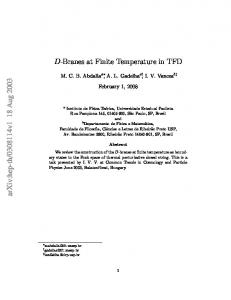
FIG. 1. The Nf = 3 pQCD pressure specified in Eq. (1) as a function of the temperature. Successive perturbative approximations are shown through order α3s ln αs for vanishing µ (left) and for non-vanishing µ (right). The p shaded bands indicate the variation of the pressure as the MS renormalisation scale is varied around a central value of Λ = 2π T 2 + µ2 /π 2 [17, 19] by a factor of two. We use ΛMS = 290 MeV based on recent lattice calculations [20] of the three-loop running of αs .
"
� F6 = − 659.175 + 65.888 − 341.489 µ ˆ2 + 1446.514 µ ˆ 4 Nf
� + 7.653 + 16.225 µ ˆ2 − 516.210 µ ˆ4 Nf2 # � � �� � � � � 1 + 12ˆ µ2 2 1 + 12ˆ µ2 αs 1485 2 ˆ 1+ 1 − Nf log Λ log 1+ Nf Nf 4π − 2 6 33 π 6 hα i s −475.587 log 4π 2 CA , π
(7)
where here and throughout all hatted quantities are scaled by 2πT , e.g. µ ˆ = µ/(2πT ), Λ is the modified minimum ˆ is the running coupling. At finite T the central value subtraction (MS) renormalisation scale, and αs = αs (Λ) of the renormalisation scale is usually chosen to be 2πT . However, at finite T and µ we use the central scale p Λ = 2π T 2 + (µ/π)2 , which is the geometric mean between 2πT and 2µ [17, 19]. In Fig. 1 we plot the ratio of the pressure to an ideal gas of quarks and gluons. The figure clearly demonstrates the poor convergence of the naive perturbative series and the increasing sensitivity of the result to the renormalisation scale as successive orders in the weak coupling expansion are included. The slow convergence found when naively applying pQCD has led to various resummation schemes which attempt to improve the convergence of the successive approximations by reorganizing the calculation in terms of quasiparticle degrees of freedom [21–37]. These resummation methods include some relevant physical ingredients, e.g. screening masses and Landau damping. These reorganisations of perturbation theory canonically include quasiparticle degrees of freedom from the outset, as opposed to naive perturbation theory. In the naive perturbative treatment an expansion around the vacuum is made and one only includes quasiparticle effects in order to regulate infrared divergenences. Based on Hard Thermal Loop (HTL) resummation [22, 23], a manifestly gauge-invariant reorganization of finite temperature/density QCD called HTL perturbation theory (HTLpt) has been developed [29]. HTLpt has so far been applied primarily to the case of finite temperature and zero chemical potential. In HTLpt [29] the next-to-leading order (NLO) [30] and next-to-next-to-leading order (NNLO) [31] thermodynamic functions have been calculated at finite T but µ = 0. Recently [33, 36] the leading order (LO) HTL pressure for finite T and µ has been calculated and approximately a decade ago it was applied at LO for finite µ but T = 0 [37]. In view of the ongoing RHIC beam energy scan and planned FAIR experiments, one is motivated to reliably determine the thermodynamic functions at finite chemical potential. In this article we compute the NLO pressure of quarks and gluons at finite T and µ. The computation utilizes a high temperature expansion through fourth order in
4 the ratio of the chemical potential to temperature. This allows us to reliably access the region of high temperature and small chemical potential. We compare our final result for the NLO HTLpt pressure at finite temperature and chemical potential with state-of-the-art perturbative quantum chromodynamics (QCD) calculations and available lattice QCD results. The paper is organised as follows. In Sec. II, we will briefly review HTLpt. In Sec. III we discuss various quantities required to be calculated at finite chemical potential based on prior calculations of the NLO thermodynamic at zero chemical potential [30]. In Sec. IV we reduce the sum of various diagrams to scalar sum-integrals. A high temperature expansion is made in Sec. V to obtain analytic expressions for both the LO and NLO thermodynamic potential. We then use this to compute the pressure in Sec.VI. We conclude in Sec. VII. Finally, in Appendices A and B we collect the various integrals and sum-integrals necessary to obtain the results presented in the main body of the text. II.
HARD THERMAL LOOP PERTURBATION THEORY
HTL perturbation theory [29–31] is a reorganization of the perturbation series for hot and dense QCD which has the following Lagrangian density L = (LQCD + LHTL ) √ + ∆LHTL , (8) g→ δg
where ∆LHTL collects all necessary renormalization counterterms and LHTL is the HTL effective Lagrangian [22, 23]. It can be written compactly as ! � α β � � µ � y y y 1 µ 2¯ µ 2 ψ, (9) G + (1 − δ) im ψγ LHTL = − (1 − δ)mD Tr Gµα q β 2 2 (y · D) y y·D y
where D is a covariant derivative operator, y = (1, y) is a light like vector and h· · ·i is the average over all possible directions, yˆ, of the loop momenta. The HTL effective action is gauge invariant, nonlocal, and can generate all of the HTL n-point functions [22, 23], which are interrelated through Ward identities. The mass parameters mD and mq are the Debye screening and quark masses in a hot and dense medium, respectively, which depend on the strong coupling g, temperature T , and the chemical potential µ. In the high temperature limit the leading-order expressions for mD and mq are � � g2 � Nf � 2 3Nf 2 m2D = Nc + T + , (10) µ 3 2 2π 2 � � g 2 Nc2 − 1 µ2 m2q = (11) T2 + 2 . 4 4Nc π We will not assume these expressions a priori, but instead treat mD and mq as free parameters to be fixed at the end of the calculation. In order to make the calculation tractable we make expansions in mD and mq in (9) treating the masses as order g [29–31]. The nth loop order in the HTLpt loop expansion is obtained by expanding the partition function through order δ n−1 and then taking δ → 1 [29–35]. In this work, we will fix the parameters mD and mq by employing a variational prescription which requires that the first derivative of the thermodynamic potential with respect to both mD and mq vanishes, such that the free energy is minimized. In the following, we generalize the NLO thermodynamic potential calculation from the case of zero chemical potential [30] to finite chemical potential. III.
INGREDIENTS FOR THE NLO THERMODYNAMIC POTENTIAL IN HTLPT
The LO HTLpt thermodynamic potential, ΩLO , for an SU (Nc ) gauge theory with Nf massless quarks in the fundamental representation can be written as [29, 30] ΩLO = dA Fg + dF Fq + ∆0 E0 ,
(12)
where dF = Nf Nc and dA = Nc2 − 1 with Nc is the number colour. Fq and Fg are the one loop contributions to quark and gluon free energies, respectively. The LO counterterm is the same as in the case of zero chemical potential [29] ∆0 E0 =
dA m4 . 128π 2 ǫ D
(13)
5
Σ
Fqct
Fq
F3qg
F4qg
FIG. 2. Diagrams containing fermionic lines relevant for NLO thermodynamics potential in HTLpt with finite chemical potential. Shaded circles indicate HTL n-point functions.
At NLO one must consider the diagrams shown in Fig. 2. The resulting NLO HTLpt thermodynamic potential can be written in the following general form [30] ΩNLO = ΩLO + dA [F3g + F4g + Fgh + Fgct ] + dA sF [F3qg + F4qg ] ∂ ∂ +dF Fqct + ∆1 E0 + ∆1 m2D ΩLO + ∆1 m2q ΩLO , 2 ∂mD ∂m2q
(14)
where sF = NF /2. At NLO the terms that depend on the chemical potential are Fq , F3qg , F4qg , Fqt , ∆1 m2q , and ∆1 m2D as displayed in Fig. 2. The other terms, e.g. Fg , F3g , F4g , Fgh and Fgct coming from gluon and ghost loops remain the same as the µ = 0 case [30]. We also add that the vacuum energy counterterm, ∆1 E0 , remains the same as the µ = 0 case whereas the mass counterterms, ∆1 m2D and ∆1 m2q , have to be computed for µ 6= 0. These counterterms are of order δ. This completes a general description of contributions one needs to compute in order to determine NLO HTLpt thermodynamic potential at finite chemical potential. We now proceed to the scalarization of the necessary diagrams. IV.
SCALARIZATION OF THE FERMIONIC DIAGRAMS
The one-loop quark contribution coming from the first diagram in Fig. 2 can be written as � � 2 Z Z Z X X X AS − A20 , log log P 2 − 2 log det [P / − Σ(P )] = −2 Fq = − P2 {P }
{P }
(15)
{P }
where m2q TP , iP0 m2q AS (P ) = |p| + [1 − TP ] , |p| A0 (P ) = iP0 −
(16) (17)
and TP is defined by the following integral [30] TP =
�
P02 2 P0 + p2 c2
�
c
ω(ǫ) = 2
Z1
dc(1 − c2 )−ǫ
−1
iP0 · iP0 − |p|c
(18)
In three dimensions ǫ → 0 and (18) reduces to TP =
iP0 + |p| iP0 log , 2|p| iP0 − |p|
(19)
with P ≡ (P0 , p). In practice, one must use the general form and only take the limit ǫ → 0 after renormalization.
6 The HTL quark counterterm at one-loop order can be rewritten from the second diagram in Fig. 2 as Z X P 2 + m2q . Fqct = −4 A2S − A20
(20)
The two-loop contributions coming from the third and fourth diagrams in Fig. 2 are given, respectively, by Z 1 X F3qg = g 2 Tr [Γµ (P, Q, R)S(Q) × Γν (P, Q, R)S(R)] ∆µν (P ) , 2
(21)
{P }
{P Q}
F4qg
Z 1 X Tr [Γµν (P, −P, Q, Q)S(Q)] ∆µν (P ) , = g2 2
(22)
{P Q}
where S is the quark propagator and ∆µν is the gluon propagator. Γµ and Γµν are HTL-resummed 3- and 4-point functions. Details concerning the HTL n-point functions can be found in Refs. [29, 30]. In general covariant gauge, the sum of (21) and (22) reduces to Z ( � � 1 2X F3qg+4qg = g ∆X (P )Tr Γ00 S(Q) − ∆T (P )Tr [Γµ S(Q)Γµ S(R′ )] 2 {P Q}
�
0
0
′
� +∆X (P )Tr Γ S(Q)Γ S(R )
)
,
(23)
where ∆T is the transverse gluon propagator, ∆X is a combination of the longitudinal and transverse gluon propagators [30], and R′ = Q − P . After performing the traces of the γ-matrices one obtains [30] ( Z X ˆ ·ˆrAS (Q)AS (R) − A0 (Q)A0 (R) 1 q 2 F3qg+4qg = −g 2(d − 1)∆T (P ) 2 2 AS (Q) − A0 (Q) A2S (R) − A20 (R) {P Q}
A0 (Q)A0 (R) + AS (Q)AS (R)ˆ q ·ˆr A2S (R) − A20 (R) + * ˆ 1 A0 (Q) − As (Q)ˆ q·y 2 −4mq ∆X (P ) (P ·Y )2 − (Q·Y )2 (Q·Y ) y ˆ * � 2 8mq ∆T (P ) ˆ )(A0 (R) − AS (R)ˆr · y ˆ) (A0 (Q) − AS (Q)ˆ q·y + 2 AS (R) − A20 (R) (Q·Y )(R·Y ) y ˆ * +) 4m2q ∆X (P ) ˆ − A0 (Q)A0 (R) − AS (Q)AS (R)ˆ 2A0 (R)AS (Q)ˆ q·y q ·ˆr + 2 AS (R) − A20 (R) (Q·Y )(R·Y ) −2∆X (P )
y ˆ
+O(g 2 m4q ) ,
(24)
where A0 and AS are defined in (16) and (17), respectively. We add that the exact evaluation of two-loop free energy could be performed numerically and would involve 5-dimensional integrations; however, one would need to be able to identify all divergences and regulate the numerical integration appropriately. Short of this, one can calculate the sum-integrals by expanding in a power series in mD /T , mq /T , and µ/T in order to obtain semi-analytic expressions. V.
HIGH TEMPERATURE EXPANSION
As discussed above, we make an expansion of two-loop free energies in power series of mD /T and mq /T to obtain a series which is nominally accurate to order g 5 . The HTL n-point functions can have both hard and soft momenta scales on each leg. At one-loop order the contributions can be classified “hard” or “soft” depending on whether the loop momenta are order T or gT , respectively; however, since the lowest fermonic Matsubara mode corresponds to P0 = πT , fermion loops are always hard. The two-loop contributions to the thermodynamic potential can be grouped into hard-hard (hh), hard-soft (hs), and soft-soft (ss) contributions. However, we note that one of the momenta contributing is always hard since it corresponds to a fermionic loop and therefore there will be no two-loop soft-soft contribution. Below we calculate the various contributions to the sum-integrals presented in Sec. IV.
7 A.
One-loop sum-integrals
The one-loop sum-integrals (15) and (20) correspond to the first two diagrams in Fig. 2. They represent the leadingorder quark contribution and order-δ HTL counterterm. We will expand the sum-integrals through order m4q taking mq to be of (leading) order g. This gives a result which is nominally accurate (at one-loop) through order g 5 . 1 1.
Hard Contribution
The hard contribution to the one-loop quark self-energy in (15) can be expanded in powers of m2q as # Z Z Z " 2 X X X 1 2 1 2TP (TP ) 2 2 (h) 4 log P − 4mq Fq = −2 + 2mq − 2 2+ 2 2− 2 2 . P2 P4 p P p P p P0 {P }
{P }
(25)
{P }
Note that the function TP does not appear in m2q term. The expressions for the sum-integrals in (25) are listed in Appendix A. Using those expressions, the hard contribution to the quark free energy becomes �2ǫ 2 2 � � � � � mq T 120 2 240 4 Λ 7π 2 4 1 + 12ˆ µ2 T 1+ µ ˆ + µ ˆ + Fq(h) = − 180 7 7 4πT 6 � �� ′ � ζ (−1) + ǫ 2 − 2 ln 2 + 2 + 24(γ + 2 ln 2) µ ˆ 2 − 28 ζ(3) µ ˆ4 + O µ ˆ6 ζ(−1) 4 mq (π 2 − 6) . (26) + 12π 2 Expanding the HTL quark counterterm in (20) one can write � Z Z � X X 1 2 1 2 1 (h) 2 4 2 Fqct = 4mq − 4mq − 2 2 + 2 2 TP − 2 2 (TP ) , P2 P4 p P p P p P0 {P }
(27)
{P }
where the expressions for various sum-integrals in (27) are listed in Appendix A. Using those expressions, the hard contribution to the HTL quark counterterm becomes (h)
Fqct = −
� m4q m2q T 2 1 + 12ˆ µ2 − 2 (π 2 − 6) . 6 6π
(28)
We note that the first term in (28) cancels the order-ǫ0 term in the coefficient of m2q in (26). There are no soft contributions either from the leading-order quark term in (15) or from the HTL quark counterterm in (20). B.
Two-loop sum-integrals
Since the two-loop sum-integrals given in (23) contain an explicit factor of g 2 , we only require an expansion to order m2q mD /T 3 and m3D /T 3 in order to determine all terms contributing through order g 5 . We note that the soft scales are given by mq and mD whereas the hard scale is given by T , which leads to two different phase-space regions as discussed in Sec. V A. In the hard-hard region, all three momenta P , Q, and R are hard whereas in the hard-soft region, two of the three momenta are hard and the other one is soft. 1.
The hh contribution
The self-energies for hard momenta are suppressed [22, 23, 30] by m2D /T 2 or m2q /T 2 relative to the propagators. For hard momenta, one just needs to expand in powers of gluon self-energies ΠT , ΠL , and quark self-energy Σ. So,
1
Of course, this won’t reproduce the full g 5 pQCD result in the limit g → 0. In order to reproduce all known coefficients through O(g 5 ), one would need to perform a NNLO HTLpt calculation.
8 the hard-hard contribution of F3qg and F4qg in (23) can be written as � Z � Z Z X X X 1 1 1 1 d−2 1 (hh) 2 2 2 −2 TP + 4 2 − F3qg+4qg = (d − 1)g + 2mD g P 2 Q2 P 2 Q2 p2 P 2 Q 2 P Q d − 1 p2 P 2 Q 2 P {Q}
P {Q}
{P Q}
� Z � X 1 q2 4d 2d P · Q d+1 TR − − + m2D g 2 d − 1 P 2 Q2 r 2 d − 1 P 2 Q2 r 4 d − 1 P 2 Q2 r 4 {P Q}
+ m2D g 2
� Z � X 3−d 1 1 q2 q2 2d P · Q d+2 4d 4 + − + − d − 1 P 2 Q2 R 2 d − 1 P 2 Q2 r 4 d − 1 P 2 Q2 r 2 d − 1 P 2 Q2 r 4 d − 1 P 2 Q2 r 2 R 2
{P Q}
+
2m2q g 2 (d
Z � X
− 1)
{P Q}
� � Z � X p2 − r 2 2 1 1 2 2 + 2 2 2 2 TQ + 2mq g (d − 1) − 2 2 2 TQ P 2 Q20 Q2 q P Q0 R P 2 Q4 P Q0 Q
� Z � X 1 2 p2 − r 2 d+3 2 2 − 2 4− 2 2 2 2 , + 2mq g (d − 1) d − 1 P 2 Q2 R 2 P Q q P Q R
P {Q}
(29)
{P Q}
where the various sum-integrals are evaluated in Appendices A and B. Using those sum-integral expressions, the hh contribution becomes � � 5π 2 αs 4 72 2 144 4 (hh) F3qg+4qg = T 1+ µ ˆ + µ ˆ 72 π 5 5 � � �4ǫ " 1 + 6(4 − 3ζ(3)) µ ˆ2 − 120(ζ(3) − ζ(5)) µ ˆ4 + O µ ˆ6 Λ 1 αs − 72 π 4πT ǫ i � + 1.3035 − 59.9055 µ ˆ2 − 75.4564 µ ˆ4 + O µ ˆ6 m2D T 2 � �4ǫ � � � 1 αs Λ 1 − 12 µ ˆ2 2 4 6 + m2q T 2 . (30) + 8.9807 − 152.793 µ ˆ + 115.826 µ ˆ +O µ ˆ 8 π 4πT ǫ 2.
The hs contribution
Following Ref. [30] one can extract the hard-soft contribution from (23) as the momentum P is soft whereas momenta Q and R are always hard. The function associated with the soft propagator ∆T (0, p) or ∆X (0, p) can be expanded in powers of the soft momentum p. For ∆T (0, p), the resulting integrals R over p are not associated with any scale and they vanish in dimensional regularization. The integration measure p scales like m3D , the soft propagator ∆X (0, p) scales like 1/m2D , and every power of p in the numerator scales like mD . The contributions that survive only through order g 2 m3D T and m2q mD g 3 T from F3qg and F4qg in (23) are (hs)
F3qg+4qg = g 2 T
Z
p
� � Z Z � Z � X X 1 1 2 4q 2 1 2(3 + d) q 2 8 q4 2 2 + 2m g T − − + D 2 2 p2 + m2D Q2 Q4 Q4 d Q6 d Q8 p p + mD
−4m2q g 2 T
{Q}
Z
p
p2
1 + m2D
{Q}
� �# Z " X 3 4q 2 4 2 1 . − 6 − 4 TQ − 2 Q4 Q Q Q (Q·Y )2 yˆ
(31)
{Q}
Using the sum-integrals contained in Appendices A and B, the hard-soft contribution becomes � � � αs 1 1 (hs) 3 2 2 4 6 ˆ )+ + 1 + 2γ + 4 ln 2 − 14ζ(3) µ ˆ + 62ζ(5) µ ˆ +O µ ˆ F3qg+4qg = − αs mD T (1 + 12 µ 6 24π 2 ǫ �2ǫ � �2ǫ � Λ αs Λ m3D T − 2 m2q mD T . × 4πT 2mD 2π
(32)
9 3.
The ss contribution
As discussed earlier in Sec. V there is no soft-soft contribution from the diagrams in Fig. 2 involving since at least one of the loops is fermionic. C.
Thermodynamic potential
Now we can obtain the HTLpt thermodynamic potential Ω(T, µ, αs , mD , mq , δ) through two-loop order for which the contributions involving quark lines are computed here whereas the ghost and gluon contributions are computed in Ref. [30]. We also follow the same prescription as in Ref. [30] to determine the mass parameter mD and mq from respective gap equations but with finite quark chemical potential, µ. 1.
Leading order thermodynamic potential
Using the expressions of Fq with finite quark chemical potential in (26) and Fg from Ref. [30], the total contributions from the one-loop diagrams including all terms through order g 5 becomes ( " !# � � ˆ π2 T 4 7 dF ζ ′ (−1) 120 2 240 4 15 Λ Ωone loop = −dA 1+ 1+ǫ 2+2 m ˆ 2D 1+ µ ˆ + µ ˆ − + 2 ln 45 4 dA 7 7 2 ζ(−1) 2 !# " ′ ˆ � � ζ (−1) Λ dF m ˆ 2q + 2 ln + 24(γ + 2 ln 2)ˆ µ2 − 28ζ(3)ˆ µ4 + O µ ˆ6 1 + 12ˆ µ2 + ǫ 2 − 2 ln 2 + 2 − 30 dA ζ(−1) 2 ) ! � �2ǫ � � ˆ Λ dF 2 8 45 1 Λ 2π 2 4 4 3 + 30 (33) m ˆ D − 60 (π − 6)m 1+ ǫ m ˆq , ˆD + + 2 ln − 7 + 2γ + 2mD 3 8 ǫ 2 3 dA ˆ and µ where m ˆ D, m ˆ q , Λ, ˆ are dimensionless variables: mD 2πT mq m ˆq = 2πT ˆ= Λ Λ 2πT µ µ ˆ= 2πT
m ˆD =
,
(34)
,
(35)
,
(36)
.
(37)
Adding the counterterm in (13), we obtain the thermodynamic potential at leading order in the δ-expansion: ( " !# � � ˆ 7 dF ζ ′ (−1) Λ 15 120 2 240 4 π2 T 4 1+ 1+ǫ 2+2 m ˆ 2D µ ˆ + µ ˆ − + 2 ln 1+ ΩLO = −dA 45 4 dA 7 7 2 ζ(−1) 2 !# " ˆ � � dF ζ ′ (−1) Λ 2 2 4 6 − 30 m ˆ 2q 1 + 12ˆ µ + ǫ 2 − 2 ln 2 + 2 + 2 ln + 24(γ + 2 ln 2)ˆ µ − 28ζ(3)ˆ µ +O µ ˆ dA ζ(−1) 2 ) ! �2ǫ � � � 2 ˆ Λ d 8 45 2π Λ F (38) 2 ln − 7 + 2γ + m ˆ 4D − 60 (π 2 − 6)m 1+ ǫ m ˆ 4q , ˆ 3D + + 30 2mD 3 8 2 3 dA where we have kept terms of O(ǫ) since they will be needed for the two-loop renormalization. 2.
Next-to-leading order thermodynamic potential
The complete expression for the next-to-leading order correction to the thermodynamic potential is the sum of the contributions from all two-loop diagrams, the quark and gluon counterterms, and renormalization counterterms.
10 Adding the contributions of the two-loop diagrams, F3qg+4qg , involving a quark line in (30) and (32) and the contributions of F3g+4g+gh from Ref. [30], one obtains � � � �� �� π 2 T 4 αs 5 5 72 2 144 4 Ωtwo loop = −dA − cA + sF 1 + + 15 cA + sF 1 + 12 µ ˆ2 m ˆD µ ˆ + µ ˆ 45 π 4 2 5 5 "� ! � ˆ �� � 4 1 Λ 55 2 4 6 cA − sF 1 + 6(4 − 3ζ(3)) µ ˆ − 120(ζ(3) − ζ(5)) µ ˆ +O µ ˆ + 4 ln − 8 11 ǫ 2 � �� �� 72 ˆ2 − 21.0214 µ ˆ4 + O µ ˆ 6 − cA − sF 0.4712 − 34.8761 µ ln m ˆ D − 1.96869 m ˆ 2D 11 # " ! ˆ � � 1 Λ 45 ˆ 2q + 8.9807 − 152.793 µ ˆ2 + 115.826 µ ˆ4 + O µ ˆ6 m ˆ2 sF 1 − 12 µ + 4 ln − 2 ǫ 2 "� ! � � � ˆ 165 27 4 1 Λ 2 + 180sF m ˆ Dm ˆq + cA − sF + 4 ln − 2 ln m ˆ D + cA + 2γ 4 11 ǫ 2 11 � � �� 4 (39) m ˆ 3D , ˆ2 + 62ζ(5) µ ˆ4 + O µ ˆ6 sF 1 + 2γ + 4 ln 2 − 14ζ(3) µ − 11 where cA = Nc and sF = Nf /2. The HTL gluon counterterm is the same as obtained at zero chemical potential [30] " ! # ˆ π 2 T 4 15 2 Λ 45 1 2π 2 4 3 Ωgct = −dA m ˆD , m ˆ D − 45m ˆD − + 2 ln − 7 + 2γ + 45 2 4 ǫ 2 3
(40)
The HTL quark counterterm as given by (28) is Ωqct = −dF
� π2 T 4 � 30(1 + 12 µ ˆ2 ) m ˆ 2q + 120(π 2 − 6) m ˆ 4q . 45
(41)
The ultraviolet divergences that remain after adding (39), (40), and (41) can be removed by renormalization of the vacuum energy density E0 and the HTL mass parameter mD and mq . The renormalization contributions [30] at first order in δ are ∆Ω = ∆1 E0 + ∆1 m2D
∂ ∂ ΩLO + ∆1 m2q ΩLO . ∂m2D ∂m2q
(42)
The counterterm ∆1 E0 at first order in δ will be same as the zero chemical potential counterterm ∆1 E0 = −
dA m4 . 64π 2 ǫ D
The mass counterterms necessary at first order in δ are found to be � � �� � αs 11 m ˆ 2D ∆1 m ˆ 2D = − cA − sF − sF (1 + 6m ˆ D ) (24 − 18ζ(3))ˆ µ2 + 120(ζ(5) − ζ(3))ˆ µ4 + O µ ˆ6 3πǫ 4
(43)
(44)
and
∆1 m ˆ 2q
� � αs 9 dA 1 − 12 µ ˆ2 2 =− m ˆ . 3πǫ 8 cA 1 + 12 µ ˆ2 q
(45)
Using the above counterterms, the complete contribution from the counterterms in (42) at first order in δ at finite chemical potential becomes π2 T 4 45
� � � �� � 4 45 4 αs 55 cA − sF 1 + (24 − 18ζ(3))ˆ µ2 + 120(ζ(5) − ζ(3))ˆ µ4 + O µ ˆ6 m ˆD + 4ǫ π 8 11 ! ! � � ′ ˆ ˆ 165 4 1 ζ (−1) Λ Λ 1 2 m ˆD − cA − sF ˆ 3D +2+2 + 2 ln + 2 + 2 ln − 2 ln m ˆD m ǫ ζ(−1) 2 4 11 ǫ 2
∆Ω = −dA
�
11 � � ′ �� � ζ (−1) 165 4 ˆ 3D 2 µ2 + 120(ζ(5) − ζ(3))ˆ µ4 + O µ ˆ6 sF (24 − 18ζ(3))ˆ + 2 ln m ˆD m 4 11 ζ(−1) ˆ ˆ2 ˆ2 1 + 12 µ Λ ζ ′ (−1) 45 1 − 12 µ sF + 2 + 2 ln − 2 ln 2 + 2 + 24(γ + 2 ln 2) µ ˆ2 + 2 1 + 12 µ ˆ2 ǫ 2 ζ(−1) ! #) � 4 6 . m ˆ 2q − 28ζ(3) µ ˆ +O µ ˆ −
(46)
Adding the contributions from the two-loop diagrams in (39), the HTL gluon and quark counterterms in (40) and (41), the contribution from vacuum and mass renormalizations in (46), and the leading-order thermodynamic potential in (38) we obtain the complete expression for the QCD thermodynamic potential at next-to-leading order in HTLpt: ( ! � � ˆ 7 dF Λ 45 π2 T 4 120 2 240 4 7 π2 3 1+ log − + γ + m ˆ 4D ˆD − 1+ ΩNLO = −dA µ ˆ + µ ˆ − 15m 45 4 dA 7 7 4 2 2 3 " � � �� � � 4 αs dF 2 5 5 72 2 144 4 + 60 − cA + sF 1 + + 15 cA + sF (1 + 12ˆ µ2 ) m ˆD µ ˆ + µ ˆ π −6 m ˆq + dA π 4 2 5 5 ( " ! ! ˆ ˆ 55 Λ Λ 36 4 − cA log − log − 2.337 log m ˆ D − 2.001 − sF 4 2 11 11 2 #) ! ! ˆ ˆ � Λ Λ 2 4 6 m ˆ 2D ˆ + 120 (ζ(5) − ζ(3)) log − 1.0811 µ ˆ +O µ ˆ + (24 − 18ζ(3)) log − 15.662 µ 2 2 ( ) ! ˆ ˆ � Λ Λ 2 4 6 − 45 sF log + 2.198 − 44.953ˆ m ˆ 2q µ − 288 ln + 19.836 µ ˆ +O µ ˆ 2 2 ( !) ! ˆ ˆ � Λ Λ 5 4 1 165 2 4 6 cA log + m ˆ 3D + γ − sF log − + γ + 2 ln 2 − 7ζ(3)ˆ µ + 31ζ(5)ˆ µ +O µ ˆ + 2 2 22 11 2 2 #) � ′ � �� 3 � ζ (−1) 2 2 4 6 + 15sF 2 m ˆ D + 180 sF m ˆ Dm ˆ q .(47) µ + 120(ζ(5) − ζ(3))ˆ µ +O µ ˆ + 2 ln m ˆ D (24 − 18ζ(3))ˆ ζ(−1) VI.
PRESSURE
In the previous section we have computed both LO and NLO thermodynamic potential in presence of quark chemical potential and temperature. All other thermodynamic quantities can be calculated using standard thermodynamic relations. The pressure is defined as P = −Ω(T, µ, mq , mD ) ,
(48)
where mD and mq are determined by requiring ∂ΩNLO = 0, ∂m ˆD ∂ΩNLO = 0. ∂m ˆq This leads to the following two gap equations which will be solved numerically # ! ( " ! " ˆ ˆ αs Λ 55 7 π2 36 Λ 2 2 m ˆD = 15(cA + sF (1 + 12ˆ µ )) − cA ln − ln m ˆ D − 3.637 45m ˆ D 1 + ln − + γ + 2 2 3 π 2 2 11 ( ! ˆ ˆ 4 Λ Λ − sF ln − 2.333 + (24 − 18ζ(3)) ln − 15.662 µ ˆ2 11 2 2 " ! )# ! ˆ ˆ Λ 495 5 Λ 4 m ˆD + cA ln + ˆ +γ +120(ζ(5) − ζ(3)) ln − 1.0811 µ 2 2 2 22
(49)
12
2 - loop Αs ; L
MS
1.2
= 268 MeV , Μ = 0
1.0
1.0
0.8
0.8
P Pideal
P Pideal
1.2
0.6
2 - loop Αs ; L
MS
= 268 MeV , Μ = 200 MeV
0.6 0.4
0.4 LO HTLpt
LO HTLpt
0.2
NLO HTLpt
0.2
NLO HTLpt
Α s 3 lnΑ s pQCD
0.0 200
10 3
10 4
Α s 3 lnΑ s pQCD
10 5
0.0 200
10 3
10 4
10 5
T H MeV L
T H MeV L
FIG. 3. The NLO HTLpt pressure scaled with ideal gas pressure plotted along with four-loop pQCD pressure [17] for two different values of chemical potential with Nf = 3 and 2-loop running coupling p constant αs . The bands are obtained by varying the renormalisation scale by a factor of 2 around its central value Λ = 2π T 2 + µ2 /π 2 [17, 19]. We use ΛMS = 290 MeV based on recent lattice calculations [20] of the three-loop running of αs .
( ˆ Λ 1 4 µ2 + 31ζ(5)ˆ µ4 − sF ln − + γ + 2 ln 2 − 7ζ(3)ˆ 11 2 2 ) � ′ �� � � ζ (−1) 1 2 2 2 4 − mD + 180sF m ˆq , (24 − 18ζ(3))ˆ µ + 120(ζ(5) − ζ(3))ˆ µ + ln mD + ζ(−1) 3
(50)
and m ˆ 2q
dA αs sF = 8dF (π 2 − 6) π
"
ˆ Λ 3 ln + 2.198 − 44.953 µ ˆ2 − 2
# ! ! ˆ Λ 4 ˆD . 288 ln + 19.836 µ ˆ − 12m 2
(51)
For convenience and comparison with lattice data [6], we define the pressure difference ∆P (T, µ) = P (T, µ) − P (T, 0) .
(52)
In Figs. 3 and 4 we present a comparison of NLO HTLpt pressure with that of four-loop pQCD [17] as a function of the temperature for two and three loop running of αs . The NLO HTLpt result differs from the pQCD result through order α3s ln αs at low temperatures. A NNLO HTLpt calculation at finite µ would agree better with pQCD α3s ln αs as found in µ = 0 case [31]. The HTLpt result clearly indicates a modest improvement over pQCD in respect of convergence and sensitivity of the renormalisation scale. In Fig. 5 the pressure difference, ∆P , is also compared with the same quantity computed using pQCD [17] and lattice QCD [6]. Both LO and NLO HTLpt results are less sensitive to the choice of the renormalisation scale than the weak coupling results with the inclusion of successive orders of approximation. Comparison with available lattice QCD data [6] suggests that HTLpt and pQCD cannot accurately account for the lattice QCD results below approximately 3 Tc ; however, the results are in very good qualitative agreement with the lattice QCD results without any fine tuning. VII.
CONCLUSIONS AND OUTLOOK
In this paper we have generalized the zero chemical potential NLO HTLpt calculation of the QCD thermodynamic potential [30] to finite chemical potential. We have obtained (semi-)analytic expressions for the thermodynamic
13
3 - loop Αs ; L
MS
1.2
= 290 MeV , Μ = 0
1.0
1.0
0.8
0.8
P Pideal
P Pideal
1.2
0.6 0.4
3 - loop Αs ; L
MS
= 290 MeV , Μ = 200 MeV
0.6 0.4 LO HTLpt
LO HTLpt
0.2
0.2
NLO HTLpt
NLO HTLpt Α s 3 lnΑ s pQCD
3
Α s lnΑ s pQCD
0.0 200
10 3
10 4
0.0 200
10 5
10 3
T H MeV L
10 4
10 5
T H MeV L
FIG. 4. Same as Fig. 3 but for 3-loop αs .
µB=100 MeV; αs3lnαs pQCD NLO HTLpt Free lattice µB=200 MeV; αs3lnαs pQCD NLO HTLpt Free lattice µB=300 MeV; αs3lnαs pQCD NLO HTLpt Free lattice
0.3
∆ P/T4
0.25 0.2
0.3 0.25
2-loop αs ; Λ MS = 268 MeV
0.15
0.2
0.1
0.05
0.05
250
300
350
400
450
T(MeV)
500
550
600
3-loop αs ; Λ MS = 290 MeV
0.15
0.1
0
µB=100 MeV; αs3lnαs pQCD NLO HTLpt Free lattice µB=200 MeV; αs3lnαs pQCD NLO HTLpt Free lattice µB=300 MeV; αs3lnαs pQCD NLO HTLpt Free lattice
0.35
∆ P/T4
0.35
0
250
300
350
400
450
500
550
600
T(MeV)
FIG. 5. (Left panel) ∆P for Nf = 3 is plotted as a function of T for two-loop HTLpt result along with those of four-loop � pQCD up to α3s ln αs [17] and lattice QCD [6] up to O µ2 using 2-loop running coupling constant αs . (Right panel) Same as left panel but using 3-loop running coupling. In both cases three different values of µ are shown as specified in the legend. The bands in pboth HTLpt and pQCD are obtained by varying the renormalisation scale by a factor of 2 around its central value Λ = 2π T 2 + µ2 /π 2 [17, 19].
potential at both LO and NLO in HTLpt. The results obtained are trustworthy at high temperatures and small chemical potential since we performed an expansion in the ratio of the chemical potential over the temperature. This calculation will be useful for the study of finite temperature and chemical potential QCD matter. This is important in view of the ongoing RHIC beam energy scan and proposed heavy-ion experiments at FAIR. Using the NLO HTLpt thermodynamic potential, we have obtained a variational solution for both mass parameters, mq and mD , and we have used this to obtain the pressure at finite temperature and chemical potential. When compared with the weak coupling expansion of QCD, the HTLpt pressure helps somewhat with the problem of oscillation of
14 successive approximations found in pQCD. Furthermore, the scale variation of the NLO HTLpt result for pressure is smaller than that obtained with the weak coupling result. The HTLpt pressure shows some deviations from the lattice data below 3 Tc which suggests that the calculation should be extended to NNLO. In addition, getting better agreement with pQCD at low temperature will require going to NNLO. This is indeed a very challenging job which represents work in progress. We also note that, based on the results obtained herein, one can straightforwardly compute quark susceptibilities. In a forthcoming paper we will compare the NLO HTLpt results for quark susceptibilities with lattice data and other theoretical models of QCD matter. ACKNOWLEDGEMENTS
We thank S. Borsanyi and N. Su for useful discussions. M.S. was supported by NSF grant No. PHY-1068765. Appendix A: Sum-Integrals
In the imaginary-time (Euclidean time) formalism for the field theory of a hot and dense medium, the 4-momentum P = (P0 , p) is Euclidean with P 2 = P02 + p2 . The Euclidean energy P0 has discrete values: P0 = 2nπT for bosons and P0 = (2n + 1)πT − iµ for fermions, where n is an integer running from −∞ to ∞, µ is the quark chemical potential, and T = 1/β is the temperature of the medium. Loop diagrams usually then involve sums over P0 and integrals over p. In dimensional regularization, the integral over spatial momentum is generalized to d = 3 − 2ǫ spatial dimensions. We define the dimensionally regularized sum-integral as � γ 2 �ǫ Z X Z d3−2ǫ p X e Λ , (A.1) T ≡ 4π (2π)3−2ǫ P =2nπT 0 P � γ 2 �ǫ Z Z X X e Λ d3−2ǫ p ≡ , (A.2) T 4π (2π)3−2ǫ P0 =(2n+1)πT −iµ
{P }
where 3 − 2ǫ is the dimension of space, Λ is an arbitrary momentum scale, P is the bosonic loop momentum, and {P } is the fermionic loop momentum. The factor (eγ /4π)ǫ is introduced so that, after minimal subtraction of the poles in ǫ due to ultraviolet divergences, Λ coincides with the renormalization scale of the MS renormalization scheme. We describe below the technique of contour integration [12, 13] in the complex plane to evaluate the frequency sum over P0 . Consider a meromorphic function f (P0 ) that originates from a loop diagram, then one can write I X X dP0 β β(iP0 − µ) T β f (P0 ) = T T f (P0 ) tanh =− × × (2πi) Residues , (A.3) 2 2 2πi 2 C 2πi P0 =(2n+1)πT −iµ
provided f (P0 ) is regular in Re(iP0 ) = µ line as shown in Fig. 6. Below we demonstrate two examples, a simpler one involving only loop momentum and a complicated one involving fourth power of loop momentum and the HTL angular function, which would be relevant for evaluating sum-integrals: (i) Simpler one: � γ 2 �ǫ Z Z X 1 d3−2ǫ p e Λ = T 2 P 4π (2π)3−2ǫ {P }
=−
�
eγ Λ 4π
� 2 ǫ Z
d3−2ǫ p (2π)3−2ǫ
X
P0 =(2n+1)πT −iµ
�
nF (p) 2p
�
,
+ where nF (p) = [eβ(p−µ) + 1]−1 + [eβ(p+µ) + 1]−1 = [n− F (p) + nF (p)].
(ii) Involving HTL term:
� � 1 1 1 − 2p iP0 + p iP0 − p (A.4)
15
| P0
C −3πT
πT
−πT
3πT
µ
FIG. 6. The contour corresponding to (A.3) in complex P0 plane. The crosses are poles of the thermal weight factor which are shifted by an amount µ from the Re[P0 ] axis.
� � Z Z X X 1 1 P02 T = P P4 P 4 P02 + p2 c2 c {P }
{P }
1 1 − c2
�
+ * Z Z X 1 1 c2 X + P4 1 − c2 P 2 (P02 + p2 c2 )
�
� � X � 2 Z � Z X d 1 1 1 c − c1+2ǫ − + 2 2 2 2 2p dp P (1 − c ) p P2 c
=
�
=
�
1 1 − c2
1 2
�
=
γ
e Λ 4π
c
c
2
{P }
{P }
�ǫ Z
{P }
3−2ǫ
�
�
d p 1 d nF (p) − (2π)3−2ǫ p dp 2p
�
2
c
{P }
1+2ǫ
c −c (1 − c2 )2
� � c
eγ Λ2 4π
�ǫ Z
d3−2ǫ p (2π)3−2ǫ
�
� nF (p) . (A.5) 2p3
After performing the frequency sum, one is left with dimensionally regularised spatial momentum integration, which are also discussed in Appendix B. However, all other frequency sums can be evaluated in similar way as discussed above. 1.
Simple one loop sum-integrals
The specific fermionic one-loop sum-integrals needed are Z X
{P }
ln P 2 =
� � 120 µ ˆ2 7π 2 4 240 µ ˆ4 . T 1+ + 360 7 7
(A.6)
� �2ǫ � � � Z X � 1 ζ ′ (−1) Λ T2 2 2 4 6 1 + 12 µ ˆ + ǫ 2 − 2 ln 2 + 2 = − + 24(γ + 2 ln 2) µ ˆ − 28ζ(3) µ ˆ + O µ ˆ P2 24 4πT ζ(−1) {P }
�� � � ζ ′ (−1) ζ ′′ (−1) π2 2 2 4 6 . (A.7) − 4 ln 2 − 2 ln 2 + 4(1 − ln 2) +2 + 94.5749 µ ˆ − 143.203 µ ˆ +O µ ˆ +ǫ 4 + 4 ζ(−1) ζ(−1) 2
16 �2ǫ � � Z X �� 1 1 Λ 1 = + 2γ + 4 ln 2 − 14 ζ(3) µ ˆ2 + 62 ζ(5) µ ˆ4 + O µ ˆ6 P4 (4π)2 4πT ǫ {P }
� �� � π2 2 4 6 +ǫ 4(2γ + ln 2) ln 2 − 4γ1 + . − 71.6013 µ ˆ + 356.329 µ ˆ +O µ ˆ 4
(A.8)
� �2ǫ � � Z X Λ 4 T2 ζ ′ (−1) p2 2 1 + 12 µ ˆ + ǫ = − − 2 ln 2 + 2 + 8(3γ + 6 ln 2 − 1) µ ˆ2 P4 16 4πT 3 ζ(−1) {P }
− 28 ζ(3) µ ˆ4 + O µ ˆ6
���
.
(A.9)
� �2ǫ � �� � Z X � Λ 1 1 3 2 p2 2 4 6 . = + 2γ − + 4 ln 2 − 14 ζ(3) µ ˆ + 62 ζ(5) µ ˆ +O µ ˆ P6 (4π)2 4 4πT ǫ 3
(A.10)
{P }
� �2ǫ � � � � Z X p4 Λ 14 5T 2 ζ ′ (−1) 8 2 1 + 12 µ ˆ + ǫ = − − 2 ln 2 + 2 + 8 − + 3γ + 6 ln 2 µ ˆ2 P6 64 4πT 15 ζ(−1) 5 {P }
− 28 ζ(3) µ ˆ4 + O µ ˆ6
���
.
(A.11)
�2ǫ � � �� � Z X � 5 1 1 Λ 16 p4 2 4 6 . = + 2γ − + 4 ln 2 − 14 ζ(3) µ ˆ + 62 ζ(5) µ ˆ + O µ ˆ P8 (4π)2 4πT 8 ǫ 15
(A.12)
{P }
Z X
1 1 = p2 P 2 (4π)2
{P }
�
Λ 4πT
�2ǫ � �� 1 2 + 2 + 2γ + 4 ln 2 − 14 ζ(3) µ ˆ2 + 62 ζ(5) µ ˆ4 + O µ ˆ6 ǫ
� �� � π2 2 2 4 6 +ǫ 4 + 8 ln 2 + 4 ln 2 + 4γ + 8γ ln 2 + . − 4γ1 − 105.259 µ ˆ + 484.908 µ ˆ +O µ ˆ 4 2.
(A.13)
HTL one loop sum-integrals
We also need some more difficult one-loop sum-integrals that involve the HTL function defined in (18). The specific fermionic sum-integrals needed are �2ǫ � � � Z X �� 1 1 1 1 Λ 2 4 6 . T = + 1 + 2γ + 4 ln 2 − 14 ζ(3) µ ˆ + 62 ζ(5) µ ˆ + O µ ˆ P P4 (4π)2 4πT 2 ǫ
(A.14)
{P }
Z X
2 1 TP = 2 2 p P (4π)2
{P }
�
Λ 4πT
�2ǫ �
ln 2 + ǫ
�
� �� π2 2 4 6 + ln 2 2γ + 5 ln 2 − 14 ζ(3) µ ˆ + 62 ζ(5) µ ˆ +O µ ˆ 6 + ǫ 17.5137 − 85.398 µ ˆ2 + 383.629 µ ˆ4 + O µ ˆ6
Z X
{P }
1 1 TP = P 2 P02 (4π)2 +
�
�
Λ 4πT
�2ǫ �
���
.
(A.15)
�� 1 1 + 2 γ + 2 ln 2 − 7 ζ(3) µ ˆ2 + 31 ζ(5) µ ˆ4 + O µ ˆ6 ǫ2 ǫ
�� � π2 2 2 4 6 . + 4 ln 2 + 8γ ln 2 − 4γ1 − 71.6014 µ ˆ + 356.329 µ ˆ +O µ ˆ 4
(A.16)
17 Z X
{P }
4 1 (TP )2 = p2 P02 (4π)2
�
�2ǫ
Λ 4πT
� � 1 2 4 6 . ln 2 + (2γ + 5 ln 2) − 14 ζ(3) µ ˆ + 62 ζ(5) µ ˆ +O µ ˆ ǫ �
(A.17)
�2ǫ � � � � � Z X � 1 1 1 1 Λ 2 4 6 . (A.18) = − − 1 + 2γ + 4 ln 2 − 14 ζ(3) µ ˆ + 62 ζ(5) µ ˆ + O µ ˆ P 2 (P · Y )2 yˆ (4π)2 4πT ǫ {P }
3.
Z X
1 T2 = P 2 Q2 R 2 (4π)2
{P Q}
Z X
�
Simple two loop sum-integrals
Λ 4πT
T2 1 = P 2 Q2 r 2 (4π)2
�
{P Q}
Z X
{P Q}
�
T2 P ·Q = P 2 Q2 r 4 (4π)2
p2 T2 = − r 2 P 2 Q2 R 2 (4π)2
{P Q}
T2 p2 = 2 2 2 2 q P Q R (4π)2
Z X
{P Q}
Z X
Λ 4πT
�
Λ 4πT
r2 T2 = − q 2 P 2 Q2 R 2 (4π)2
{P Q}
�
�
�
Λ 4πT
�4ǫ
Λ 4πT
(A.19)
�4ǫ � �� � 1 ζ ′ (−1) 1 − 1 + 12ˆ µ2 + 4 − 2 ln 2 + 4 6 ǫ ζ(−1) ��
.
(A.20)
�4ǫ � �� � � � 1 1 ζ ′ (−1) 11 − 1 + 12ˆ µ2 + + 2γ − 2 ln 2 + 2 12 ǫ 3 ζ(−1)
+4 (7 + 12γ + 12 ln 2 − 3ζ(3)) µ ˆ2 − 4 (27ζ(3) − 20ζ(5)) µ ˆ4 + O µ ˆ6
{P Q}
Z X
Λ 4πT
� � µ ˆ2 28 2 4 6 . + 2(4 ln 2 + 2γ + 1) µ ˆ − ζ(3) µ ˆ +O µ ˆ ǫ 3
+ 48 (1 + γ + ln 2) µ ˆ2 − 76ζ(3) µ ˆ4 + O µ ˆ6
p2 T2 = 2 2 4 P Q r (4π)2
Z X
�4ǫ �
Λ 4πT
�4ǫ
�4ǫ � �� 1 ζ ′ (−1) − 1 − 6γ + 6 + 24 {2 + 3ζ(3)} µ ˆ2 36 ζ(−1)
��
.
� + 48(7ζ(3) − 10ζ(5)) µ ˆ4 + O(ˆ µ6 ) .
�� − 7.001 − 108.218 µ ˆ2 − 304.034 µ ˆ4 + O(ˆ µ6 ) .
−
p0 ,p
(A.23)
� � � � 12 5 1 24 1− (1 + 7ζ(3)) µ ˆ2 − (14ζ(3) − 31ζ(5)) µ ˆ4 + O µ ˆ6 72 ǫ 5 5
�4ǫ
�� + 9.5424 − 185.706 µ ˆ2 + 916.268 µ ˆ4 + O(ˆ µ6 ) .
(A.24)
� � 1 1 1 + 3(−2 + 7ζ(3)) µ ˆ2 + 6(14ζ(3) − 31ζ(5)) µ ˆ4 + O(ˆ µ6 ) 18 ǫ �� + 8.1428 + 96.9345 µ ˆ2 − 974.609 µ ˆ4 + O(ˆ µ6 ) .
PQ
Z
(A.22)
� �� 1 1� 1 − 12(1 − 3ζ(3)) µ ˆ2 + 240(ζ(3) − ζ(5)) µ ˆ4 + O µ ˆ6 72 ǫ
The generalized two loop sum-integrals can be written from [30] as Z Z Z Z X F (P )G(Q)H(R) = F (P )G(Q)H(R) − ǫ(p0 )nF (|p0 |) 2 ImF (−ip0 + ε, p) Re G(Q)H(R) {P Q}
(A.21)
p0 ,p
ǫ(p0 )nF (|p0 |) 2 ImG(−ip0 + ε, p) Re
Z
Q
H(Q)F (R)
Q
P0 =−ip0 +ε
(A.25)
P0 =−ip0 +ε
(A.26)
18 +
Z
ǫ(p0 )nB (|p0 |) 2 ImH(−ip0 + ε, p) Re
p0 ,p
+
Z
Q
Z
ǫ(p0 )nF (|p0 |) 2 ImF (−ip0 + ε, p)
p0 ,p
q0 ,q
Z
Z
−
ǫ(p0 )nF (|p0 |) 2 ImG(−ip0 + ε, p)
p0 ,p
q0 ,q
Z
Z
−
F (Q)G(R)
Z
ǫ(p0 )nB (|p0 |) 2 ImH(−ip0 + ε, p)
p0 ,p
q0 ,q
P0 =−ip0 +ε
ǫ(q0 )nF (|q0 |) 2 ImG(−iq0 + ε, q) ReH(R)
R0 =i(p0 +q0 )+ε
ǫ(q0 )nB (|q0 |) 2 ImH(−iq0 + ε, q) ReF (R) ǫ(q0 )nF (|q0 |) 2 ImF (−iq0 + ε, q) ReG(R)
R0 =i(p0 +q0 )+ε
.
(A.27)
R0 =i(p0 +q0 )+ε
After applying Eq. (A.27) and using the delta function to calculate the P0 and Q0 integrations, the sum-integral (A.23) reduces to Z Z − − + X nF (p) − n+ 1 2p q F (p) nF (q) − nF (q) = , (A.28) P 2 Q2 R 2 2p 2q ∆(p, q, r) {P Q}
pq
where n± F (p) =
1 eβ(p±µ)
and ∆(p, q, r) = p4 + q 4 + r4 − 2(p2 q 2 + q 2 r2 + p2 r2 ) = −4p2 q 2 (1 − x2 ) ,
+1
(A.29)
and using the result of Eq. (B.10), we get sum-integral (A.19) and agree with [17]. After applying Eq. (A.27), the sum-integral (A.20) reduces to 1 = −2 2 P Q2 r 2
Z X
{P Q}
Z
nF (p) 2p
Z
1 + 2 Q r2
Q
p
Z
nF (p)nF (q) 1 , 4pq r2
(A.30)
pq
+ where nF (p) = n− F (p) + nF (p) . Now using the result of 4-dimensional integrals from [30] and applying Eq. (B.3) and Eq. (B.5), we can calculate sum-integral Eq. (A.20). The sum-integrals (A.21) can be calculated in same way: Z Z Z Z X nF (p) nF (p)nF (q) p2 p2 p2 = −2 + . (A.31) P 2 Q2 r 4 2p Q2 r 4 4pq r4 {P Q}
Q
p
pq
The sum-integral (A.22) can be written as Z Z Z Z X X X P0 Q0 p2 1 1X P ·Q = + − P 2 Q2 r 4 P 2 Q2 r 4 2 P 2 Q2 r 2 P 2 Q2 r 4
(A.32)
Using Eq. (A.27) and after doing P0 and Q0 integrations, first sum-integral above reduces to Z Z − − + X nF (p) − n+ P0 Q0 F (p) nF (q) − nF (q) p q = , 2 2 4 P Q r 2p 2q r4
(A.33)
{P Q}
{P Q}
{P Q}
{P Q}
{P Q}
pq
and the result is given in Eq. (B.9). The second term and third terms sum-integrals above are linear combinations of Eq. (A.20) and Eq. (A.21). Adding all of them, we get required sum-integral. Similarly after applying Eq. (A.27), the sum-integral (A.23) reduces to � 2 � Z Z Z Z Z X nF (p) nB (p) p2 q p2 r2 1 − = + 2 r 2 P 2 Q2 R 2 p p2 Q2 R2 2p Q2 R 2 r 2 q {P Q}
p
+
Z
pq
Q
2
2
P0 =−ip 2 2
nF (p)nF (q) q r − p − q − 4pq r2 ∆(p, q, r)
p
Z
pq
Q
2
nF (p)nB (q) p + r 4pq q2
2
2
P0 =−ip 2 2
r −p −q , ∆(p, q, r)
(A.34)
19 So �
p2 + r 2 r 2 − p2 − q 2 q2 ∆(p, q, r)
�
=
p·ˆ ˆq
1 , 2q 2 ǫ
(A.35)
and �
q 2 r 2 − p2 − q 2 r2 ∆(p, q, r)
�
� q 2 (p2 + q 2 ) = − , ∆(p, q, r) x p ˆ·ˆ q x � � 1 − 2ǫ 1 1 q2 1 − 2ǫ 1 = − − 8ǫ p2 2ǫ r4 x 8ǫ p2 � 2� 1 q =− . 2ǫ r4 x �
q2 ∆(p, q, r)
Using the above angular integration, Eq. (A.34) becomes Z Z Z X p2 nB (p) r2 = r 2 P 2 Q2 R 2 p p2 Q2 R2 {P Q}
Q
p
Z
−
�
nF (p) 2p
Z
1 nF (p)nF (q) p2 − 4 4pq r 2ǫ
Z
pq
q2 p2 + r2 q2
�
1 Q2 R 2
Q
p
P0 =−ip
1 − 2ǫ
�
(A.36)
�
P0 =−ip
nF (p)nB (q) 1 . 4pq q2
Z
(A.37)
pq
Using the 4-dimensional integrals from [30] and Eqs. (B.2), (B.3), (B.4) and (B.6), we obtain the sum-integral (A.23). Similarly after applying Eq. (A.27), the sum-integral (A.24) reduces to � 2 � Z Z Z Z Z X nF (p) nB (p) p2 p q 2 q 2 1 − = + 2 q 2 P 2 Q2 R 2 p Q2 r2 R2 2p Q2 R 2 q 2 p p p Q Q {P Q} P0 =−ip P0 =−ip � 2 � 2 Z Z 2 2 2 2 2 2 nF (p)nF (q) p r − p − q nF (p)nB (q) p r r − p − q2 + + 2 − . (A.38) 2 2 4pq q ∆(p, q, r) 4pq r p ∆(p, q, r) pq
pq
Now �
p2 r 2 − p2 − q 2 q 2 ∆(p, q, r)
�
= 0,
(A.39)
p·ˆ ˆq
and ��
p2 r2 + r2 p2
�
r 2 − p2 − q 2 ∆(p, q, r)
�
1 1 1 = − 2 2ǫ p 2ǫ p·ˆ ˆq
�
p2 r4
�
.
(A.40)
x
Using the above angular average, we find Z X
p2 = q 2 P 2 Q2 R 2
{P Q}
Z
nB (p) p
Q
p
1 − 2ǫ
Z
Z
pq
q 2 Q2 r2 R2
−
Z p
P0 =−ip
nF (p)nB (q) 1 1 + 2pq p2 2ǫ
Z
nF (p) 2p
Z
1 2 Q R2
Q
nF (p)nB (q) p2 2pq r4
�
p2 q2 + q2 p2
�
P0 =−ip
(A.41)
pq
Using the 4-dimensional integrals from [30] and Eqs. (B.2), (B.3), (B.4) and (B.7), we obtain the sum-integral (A.24). Similarly after applying Eq. (A.27), the sum-integral (A.25) reduces to � 2 � Z Z Z Z Z X nF (p) nB (p) r2 r r2 p2 1 − = + 2 p2 P 2 Q 2 R 2 p Q2 r2 R2 2p Q 2 R 2 p2 q p p Q Q {P Q} P0 =−ip P0 =−ip � � 2 Z Z nF (p)nF (q) r2 r2 − p2 − q 2 nF (p)nB (q) q 2 q2 r − p2 − q 2 + + 2 − . (A.42) 4pq p2 ∆(p, q, r) 4pq r2 p ∆(p, q, r) pq
pq
20 Now �
r 2 r 2 − p2 − q 2 p2 ∆(p, q, r)
�
and ��
q2 q2 + r2 p2
�
r 2 − p2 − q 2 ∆(p, q, r)
Using the above angular average, we have Z Z Z 2 2 X nB (p) p q = q 2 P 2 Q2 R 2 p Q2 r2 R2 {P Q}
Q
p
1 + 2ǫ
p ˆ·ˆ q
�
(A.43)
�
nF (p) 2p
Z
Z p
P0 =−ip
pq
1 , 2p2 ǫ
1 =− 2ǫ p ˆ·ˆ q
−
nF (p)nB (q) 1 1 + 2 2pq p 2ǫ
Z
=
Z
q2 r4
�
.
(A.44)
x
1 Q2 R 2
Q
nF (p)nB (q) q 2 . 2pq r4
�
� p q + q2 p2 2
2
P0 =−ip
(A.45)
pq
Using the 4-dimensional integrals from [30] and Eqs. (B.2), (B.3), (B.4) and (B.8), we obtain the sum-integral (A.24). 4.
Z X
1 T2 T = R P 2 Q2 r 2 (4π)2
{P Q}
Z X
T2 p2 TR = 2 2 4 P Q r (4π)2
Z X
{P Q}
�4ǫ � �� � � 1 1 ζ ′ (−1) 1 2 − + 2 + 12(1 + 8 µ ˆ ) ln 2 + 4 48 ǫ2 ζ(−1) ǫ
�
Λ 4πT
���
.
(A.46)
�4ǫ � �� � � 1 1 ζ ′ (−1) 1 26 2 − + + 4(13 + 144 µ ˆ ) ln 2 + 4 576 ǫ2 3 ζ(−1) ǫ �� + 446.397 + 2717.86 µ ˆ2 − 1735.61 µ ˆ4 + O(ˆ µ6 ) .
P ·Q T2 T = R P 2 Q2 r 4 (4π)2
{P Q}
Λ 4πT
+ 136.3618 + 460.23 µ ˆ2 − 273.046 µ ˆ4 + O µ ˆ6
{P Q}
Z X
�
HTL two loop sum-integrals
�
Λ 4πT
(A.47)
�4ǫ � �� � � 1 1 ζ ′ (−1) 1 − + 4 ln 2 + 4 ′ + 69.1737 + 118.244 µ ˆ2 96 ǫ2 ζ (−1) ǫ +136.688 µ ˆ4 + O µ ˆ6
T2 r 2 − p2 TQ = − 2 2 2 2 P q Q0 R (4π)2
�
Λ 4πT
�4ǫ
���
.
(A.48)
� � � 1 10 1 1 ζ ′ (−1) 2 2 + 2γ + + 1 + 4 µ ˆ ln 2 + 2 2 8 ǫ ǫ 3 ζ(−1)
� � 2 (98ζ(3) − 93ζ(5)) µ ˆ4 + O µ ˆ6 3 ��� 2 . + 46.8757 − 41.1192 µ ˆ + 64.0841 µ ˆ4 + O µ ˆ6
+ 2 (8γ + 16 ln 2 − 7ζ(3)) µ ˆ2 −
(A.49)
Appendix B: Integrals 1.
Three dimensional integrals
We require one integral that does not involve the Bose-Einstein distribution function. The momentum scale in these integrals is set by the mass m = mD . The one-loop integral is � �2ǫ Z 1 Λ m [1 + 2ǫ] . (B.1) = − 2 2 4π 2m p p +m
21 2.
Λ2ǫ (4π)2
�4ǫ � � � � � � ζ ′ (−1) 1 nB (p) −2ǫ Λ T2 1 + ǫ 2 − 2 ln 2 + 4 p = p (4π)2 4πT 12 ζ(−1) � �� � � 2 ζ ′′ (−1) ζ ′ (−1) 7π +4 . − 2 + ln2 2 − 2 ln 2 + 4(1 + ln 2) 1 + + 2ǫ2 8 ζ(−1) ζ(−1)
Z p
Λ2ǫ (4π)2
Z
Z
T2 nF (p) 1 −2ǫ p = − 2p p2 (4π)2
p
Z
pq
Z
pq
�4ǫ �
(B.2)
n � ζ ′ (−1) 1 + 12ˆ µ2 + ǫ 2 − 2 ln 2 + 4 ζ(−1) � oi + 24 (2γ + 5 ln 2 − 1) µ ˆ2 − 56ζ(3) µ ˆ4 + O µ ˆ6 .
T2 nF (p) −2ǫ p = 2p (4π)2
p
Λ2ǫ (4π)2
Thermal Integrals
�
�
Λ 4πT
Λ 4πT
�4ǫ �
1 24
�h
(B.3)
� � 1 2 4 6 . (B.4) + 2 + 2γ + 10 ln 2 − 28ζ(3) µ ˆ + 124ζ(5) µ ˆ +O µ ˆ ǫ
� � � nF (p)nF (q) 1 T2 1 10 2 4 6 . = (1 − ln 2) + 4(2 ln 2 − 1)ˆ µ + ζ(3) µ ˆ +O µ ˆ 4pq r2 (4π)2 3 3 �"
(B.5)
ζ ′ (−1) − 12(−13 + 12 ln 2 + 3ζ(3))ˆ µ2 ζ(−1) # ! �� � 2 4 6 4 6 . + ǫ 3.0747 + 31.2624 µ ˆ + 262.387 µ ˆ +O µ ˆ +12 (−13ζ(3) + 20ζ(5)) µ ˆ +O µ ˆ
T2 nF (p)nF (q) p2 = 4 4pq r (4π)2
�
1 − 36
5 + 6γ + 6 ln 2 − 6
(B.6)
� "( � ζ ′ (−1) 1 7 − 6γ − 18 ln 2 + 6 − + 6(−22 + 21ζ(3)) µ ˆ2 36 ζ(−1) pq # ) �� � 2 4 6 4 6 . + ǫ 29.5113 + 158.176 µ ˆ − 557.189 µ ˆ +O µ ˆ +6 (126ζ(3) − 155ζ(5)) µ ˆ +O µ ˆ Z
Z
pq
nB (p)nF (q) p2 T2 = 2pq r4 (4π)2
nB (p)nF (q) q 2 T2 = 2pq r4 (4π)2
�
1 18
� "(
1 − 6γ − 12 ln 2 + 6
+O µ ˆ
Z
pq
� 6
)
(B.7)
ζ ′ (−1) + 12ˆ µ2 − 6 (28ζ(3) − 31ζ(5)) µ ˆ4 ζ(−1)
+ ǫ 31.0735 + 222.294 µ ˆ2 − 416.474 µ ˆ4 + O µ ˆ6
��
.
− + + �� n− T2 1 � F (p) − nF (p) nF (q) − nF (q) p q (1 − 3ζ(3)) µ ˆ2 − 20(ζ(3) − ζ(5)) µ ˆ4 + O µ ˆ6 . = 4 2 2p 2q r (4π) 3
(B.8)
(B.9)
Thermal integrals containing the triangle function: Z
pq
+ − + n− 2p q T2 F (p) − nF (p) nF (q) − nF (q) = 2p 2q ∆(p, q, r) (4π)2
�
Λ 4πT
�4ǫ �
� � µ ˆ2 28 2 4 6 . + 2(4 ln 2 + 2γ + 1) µ ˆ − ζ(3) µ ˆ +O µ ˆ ǫ 3
(B.10)
22 Thermal integrals containing both the triangle function and HTL average are listed below: � � Z �� T2 � r 2 c2 − p 2 − q 2 nF (p)nF (q) = 0.014576 + 0.238069 µ ˆ2 + 0.825164 µ ˆ4 + O µ ˆ6 . Re c2 2 4pq ∆(p + iε, q, rc) c (4π)
(B.11)
pq
Z
pq
� � 2 2 2 2 �� nF (p)nF (q) T2 � 4 r c −p −q = 0.017715 + 0.28015 µ ˆ2 + 0.87321 µ ˆ4 + O µ ˆ6 . Re c 2 4pq ∆(p + iε, q, rc) c (4π)
Z
nF (p)nF (q) Re 4pq
Z
nB (p)nF (q) Re 2pq
pq
pq
�
�
q 2 2 r 2 c2 − p 2 − q 2 c r2 ∆(p + iε, q, rc)
�
=−
c
p 2 − q 2 r 2 c2 − p 2 − q 2 r2 ∆(p + iε, q, rc)
�
c
=
(B.12)
�� T2 � 0.01158 + 0.17449 µ ˆ2 + 0.45566 µ ˆ4 + O µ ˆ6 . (B.13) 2 (4π) �� T2 � 0.17811 + 1.43775 µ ˆ2 − 2.45413 µ ˆ4 + O µ ˆ6 . (B.14) 2 (4π)
Second set of integrals involve the variables rc = |p + q/c|: � � Z 2 2 2 �� T2 � nF (p)nB (q) −1+2ǫ rc − p − q = 0.19678 + 1.07745 µ ˆ2 − 2.63486 µ ˆ4 + O µ ˆ6 . (B.15) Re c 2 2pq ∆(p + iε, q, rc ) c (4π) pq
Z
pq
� � 2 2 2 �� nF (p)nB (q) T2 � 1+2ǫ rc − p − q = Re c 0.048368 + 0.23298 µ ˆ2 − 0.65074 µ ˆ4 + O µ ˆ6 . (B.16) 2pq ∆(p + iε, q, rc ) c (4π)2 Z
pq
Z
pq
� � �4ǫ � � 2 2 2 �1 T2 1 Λ nF (p)nB (q) p2 1+2ǫ rc − p − q = 1 + 12 µ ˆ2 Re c 2 2 2pq q ∆(p + iε, q, rc ) c (4π) 4πT 96 ǫ ��� . + 7.77236 + 81.1057 µ ˆ2 − 48.5858 µ ˆ4 + O µ ˆ6
� �4ǫ � � � � nF (p)nB (q) T2 11 − 8 ln 2 1 Λ r 2 r 2 − p2 − q 2 = 1 + 12 µ ˆ2 Re c1+2ǫ c2 c 2 2pq q ∆(p + iε, q, rc ) c (4π) 4πT 288 ǫ ��� . + 7.7995 + 70.5162 µ ˆ2 − 57.9278 µ ˆ4 + O µ ˆ6
� �4ǫ � � � � 1 nF (p)nF (q) T2 1 Λ r2 − p2 rc2 − p2 − q 2 =− 1 + 12 µ ˆ2 2 Re c−1+2ǫ c 2 2 4pq q ∆(p + iε, q, rc ) c (4π) 4πT 24 ǫ pq � � � ζ ′ (−1) 2 1 + γ + ln 2 + + + (24γ + 48 ln 2 − 7ζ(3)) µ ˆ2 + (31ζ(5) − 98ζ(3)) µ ˆ4 + O µ ˆ6 ǫ ζ(−1) ��� + 40.3158 + 261.822 µ ˆ2 − 1310.69 µ ˆ4 + O µ ˆ6 .
(B.17)
(B.18)
Z
Z
pq
nB (p)nF (q) 2pq
� �4ǫ � � � 2 2 T2 1 1 rc2 − p2 − q 2 Λ −1+2ǫ rc − p =− Re c q 2 ∆(p + iε, q, rc ) c (4π)2 4πT 12 ǫ2 � � � ζ ′ (−1) 1 2 + 2γ + 4 ln 2 + 2 − 14ζ(3) µ ˆ2 + 62ζ(5) µ ˆ4 + O µ ˆ6 + ǫ ζ(−1) ��� 2 . + 52.953 − 190.103 µ ˆ + 780.921 µ ˆ4 + O µ ˆ6
(B.19)
(B.20)
23 The integral (B.12) can be evaluated directly in three dimensions at finite chemical potential. The other integrals Eqs. (B.13)–(B.20) can be evaluated following the same procedure as discussed in [30] at finite chemical potential.
[1] I. Arsene et al. (BRAHMS Collaboration), Nucl. Phys. A757, 1 (2005); K. Adcox et al. (PHENIX Collaboration), ibid. 757, 184 (2005); B. B. Back et al. (PHOBOS Collaboration), ibid. 757, 28 (2005); J. Adams et al. (STAR Collaboration), ibid. 757, 102 (2005). [2] ALICE: Physics Performance Report, Vol. I, J. Phys. G: Nucl. Part. Phys. 30, 1517 (2004); Vol. II, Phys. G: Nucl. Part. Phys. 32, 1295 (2006). [3] The CBM Physics Book, Lecture Notes in Physics 814, (B. L. Friman, C. H¨ ohne, J. E. Knoll, S. Leupold, J. Randrup, R. Rapp and P. Seneger (Eds.), Springer-Verlag, Berlin Heidelberg 2010). [4] T. DeGrand and C. DeTar, Lattice Methods for Quantum Chromodynamics, (World Scientific 2006); M. Creutz, Quarks, gluons and lattices, (Cambridge University Press 1985). [5] R. Gavai, S. Gupta, Phys. Rev. D 68, 034506 (2003). [6] Sz. Bors´ anyi, G. Endr˝ odi, Z. Fodor, S.D. Katz, S. Krieg, C. Ratti and K.K. Szab´ o, JHEP 08, 053 (2012). [7] A. Peshier, B. Kampfer, and G. Soff, Phys. Lett. B337, 235 (1994); Phys. Rev. D54, 2399(1996); Phys. Rev. C61, 045203 (2000); Phys. Rev. D66, 094003 (2002). [8] P. Braun-Munzinger, K. Redlich, J. Stachel, Quark-Gluon Plasma-3 (R. Hwa, X.N. Wang (Eds.), World Scentific, 2004) p. 491; J. Cleymans, D. Elliot, A. Keranen, E. Suhonen; Phys. Rev. C57, 3319 (1998); R. Hagedron and K. Redlich, Z. Phys. C27 541 (1985). [9] R. D. Pisarski, Phys. Rev. D62, 111501 (2000); A. Dumitru and R. D. Pisarski, Phys. Lett. B525, 95 (2002); A. Dumitru, Y. Hatta, J. Lenaghan, K. Orginos, R. D. Pisarski, Phys. Rev. D70, 034511 (2004); A. Gocksch and R. D. Pisarski, Nucl. Phys. B402, 657 (1993). [10] T. Hatsuda and T. Kunihiro, Phys. Rep. 247, 221 (1994); T. Kunihiro, Phys. Lett. B 271, 395 (1991). [11] K. Fukushima, Phys. Lett. B591, 277 (2004); Phys. Rev. D68, 045004 (2003); C. Ratti, M. A. Thaller, and W. Weise, Phys. Rev. D73, 014019; S. K. Ghosh, T. K. Mukherjee, M. G. Mustafa, and R. Ray, Phys. Rev. D 73, 114007 (2006); Phys. Rev. D 77, 094024 (2008); S. Mukherjee, M. G. Mustafa, and R. Ray, Phys. Rev. D75, 094015 (2007); S. Roessner, C. Ratti, and W. Weise, Phys. Rev. D75, 034007 (2007); C. Sasaki, B. Friman, and K. Redlich, Phys. Rev. D 75 074013 (2007); A. Bhattacharyya, P. Dev, S. K. Ghosh, and R. Ray, Phys. Rev. D 82, 014021 (2010); P. Dev, A. Lahiri, and R. Ray, Phys. Rev D82, 11402 (2010); Phys. Rev.D 83, 014011 (2010). [12] M. LeBellac, Thermal Field Theory (Cambridge University Press, Cambridge, 1996), 1st ed. [13] J. I. Kapusta and C. Gale, Finite Temperature Field Theory Principle and Applications (Cambridge University Press, Cambridge, 1996), 2nd ed. [14] E. V. Shuryak, Sov. Phys. JETP 47, 212 (1978); S.A. Chin, Phys. Lett. B78, 552 (1978); J. I. Kapusta, Nucl. Phys. B148, 461 (1997); T. Toimela, Phys. Lett. B124, 407 (1983); P. Arnold, C. X. Zhai, Phys. Rev. D50, 7603 (1994); Phys. Rev. D51, 1906 (195); C. X. Zhai and B. M. Castering, Phys. Rev. D52, 7232 (1995). [15] K. Kajantie, M. Laine, K. Rummukainen and Y. Schroder, Phys. Rev. D67, 105008 (2003) [16] A. D. Linde, Phys. Lett. B96, 289 (1980). [17] A. Vuorinen, Phys. Rev. D 67, 074032 (2003); Phys. Rev. D 68, 054017 (2003). [18] A. Ipp, K. Kajantie, A. Rebhan, and A. Vuorinen, Phys. Rev. D74, 045016 (2006). [19] A. Rebhan and P. Romatschke, Phys. Rev. D 68, 025022 (2003); W. Cassing, Nucl. Phys. A 795, 70 (2007); F. G. Gardim and F. M. Steffens, Nucl. Phys. A 825, 222 (2009); A. Kurkela, P. Romatschke and A. Vuorinen, Phys. Rev. D 81, 105021 (2010). [20] A. Bazavov et al., arXiv:1205.6155 [hep-latt] (2012). [21] F. Karsch, A. Patkos, P. Petreczky, Phys. Lett. B401, 69 (1997); S. Chiku and T. Hatsuda, Phys. Rev. D58, 076001 (19980. [22] E. Braaten and R. D. Pisarski, Nucl. Phys. B337, 569 (1990); Phys. Rev. Lett. 64, 1338 (1990). [23] E. Braaten and R. D. Pisarski, Phys. Rev. D 45, R1827 (1992). [24] J. O. Andersen, E. Braaten and M. Strickland, Phys. Rev. D 63, 105008 (2001). [25] J. O. Andersen and M. Strickland; Phys. Rev. D64, 105012 (2001). [26] J. P. Blaizot, E. Iancu, and A. Rebhan, Phys. Rev. Lett. 83, 2906 (1999); Phys. Lett. B 470, 181 (1999); Phys. Rev. D 63, 065003 (2001). [27] J.-P. Blaizot, E. Iancu, and A. Rebhan, Phys. Lett. B 523, 143 (2001); Eur. Phys. J. C 27, 433 (2003). [28] A. Peshier, Phys. Rev. D63, 105004 (2001); Nucl.Phys. A 702, 128 (2002). [29] J. O. Andersen, E. Braaten, and M. Strickland, Phys. Rev. Lett. 83, 2139 (1999); Phys. Rev. D 61, 014017 (1999); Phys. Rev. D 61, 074016 (2000). [30] J. O. Andersen, E. Petitgirard, and M. Strickland, Phys. Rev. D66 (2002) 085016; Phys. Rev. D70, 045001 (2004). [31] N. Su., J. O. Andersen, and M. Strickland, Phys. Rev. Lett. 104, 122003 (2010); J. O. Andersen, M. Strickland, and N. Su, JHEP 1008, 113 (2010); J.O. Andersen, L.E. Leganger, M. Strickland and N. Su, Phys. Lett. B 696, 468 (2011); J. O. Andersen, L. E. Leganger, M. Strickland and N. Su, JHEP 1108, 053 (2011); J. O. Andersen, L. E. Leganger, M. Strickland and N. Su, Phys. Rev. D 84, 087703 (2011).
24 [32] P. Chakraborty, M. G. Mustafa, and M. H. Thoma, Eur. Phys. J. C. 23, 591 (2002); Phys. Rev. D 68, 085012 (2003). [33] N. Haque, M. G. Mustafa and M. H. Thoma, Phys. Rev. D84, 054009 (2011); N. Haque and M. G. Mustafa, Nucl. Phys. A862-863, 271 (2011); N. Haque and M. G. Mustafa, harXiv:1007.2076 [hep-ph]i. [34] P. Chakraborty, M. G. Mustafa, and M. H. Thoma, Phys. Rev. D 67, 114004 (2003). [35] Y. Jiang, H.-x. Zhu, W.-m Sun, and H.-s. Zong, J. Phys. G 37, 055001 (2010). [36] J. O. Andersen, S. Mogliacci, N. Su and A. Vuorinen, harXiv:1210.0912 [hep-ph]i. [37] J.O. Andersen and M. Strickland, Phys. Rev. D 66, 105001 (2002).