TWO-PASS QUANTILE BASED NOISE SPECTRUM ESTIMATION Houwu Bai
Eric A. Wan
Center for Spoken Language Understanding OGI School of Science and Engineering at OHSU Email:
[email protected],
[email protected]
ABSTRACT Noise spectrum estimation from a noisy speech signal forms a critical part of such applications as single channel speech enhancement and robust automatic speech recognition (ASR). The two-pass quantile based noise estimation algorithm presented in this paper has the ability to track slow changing non-stationary noise and obtains good estimates for various noise types over a wide range of SNR levels. The essence of the two-pass approach involves first estimating the SNR for each frequency/time point using a fixed quantile value. Based on the estimated SNR, a new quantile level is chosen for each frequency subband. A second noise estimation is then performed. Application of quantile based noise estimation to a single channel speech enhancement system is used to illustrate the ability to suppress noise with little speech distortion.
1. INTRODUCTION Instantaneous noise spectrum estimation is a critical component of single channel speech enhancement and noise robust ASR systems. The simplest approach is to directly calculate the noise spectrum from the beginning segment of the noisy signal. Speech activity is assumed absent during this initial segment. This method, however, cannot be used to track non-stationary noise. A more sophisticated approach utilizes speech activity detection so that the noise estimate can be updated periodically when speech is absent. The problem with this approach is that: 1) speech activity detection in noisy environments is a difficult problem in itself; and 2) the noise estimate cannot be updated during periods of speech presence. The proposed two-pass quantile based noise estimation algorithm is developed based on previous work in [1-4]. The principle idea stems from a minimum statistic algorithm by Martin [1,2], which is based on the observation that the smoothed power estimate of a noisy speech signal exhibits distinct peaks and valleys that represent speech presence and speech absence respectively. In Martin’s algorithm, the minimum of smoothed power within a finite length window is used to estimate the noise power. To estimate the noise spectrum, one can apply the short-time discrete Fourier transform (STDFT) to the noisy speech, calculate the magnitude and then run the minimum statistic algorithm for each frequency band separately. In practice, however, the minimum statistic algorithm can be sensitive to outliers and it is also likely to underestimate the noise level.
Quantile based estimation can be viewed as a generalization of the minimum statistic approach. By definition, the quantile for a dataset {xi, i=0...N} is calculated by first sorting such that: x 0 ≤ x1 ≤ ... ≤ x N
The quantile or q-value is xint( Nq ) , where 0 ≤ q ≤ 1 and int( ) rounds to the nearest integer (q=0 corresponds to the minimum, q=1 corresponds to the maximum, and q=0.5 corresponds to the median). In [3], the median of the noisy speech spectrum was used as a more robust estimate of the noise level. The assumption is that for a certain finite length window, speech is present for less than half the duration. In [4], however, the author presented experimental results showing the probability of having more than 20% duration being silence for various segment lengths ranging from 200ms to 2000ms. For example, when the time segment length is 600ms, the probability of having more than 20% silence is greater than 85%. This indicates that the median assumption is too aggressive resulting in the increased likelihood of overestimating the noise level. Thus the authors chose a level associated with q=0.2. In addition, instead of using the quantile itself, the arithmetic mean of the lower 20% (i.e., q < 0.2) of the noisy speech power spectrum is used as the noise estimation. According to their experiments, this “low energy envelope” tracking method generally obtains better estimates compared to other published quantile methods [2,3]1, as well as alternative approaches such as Hirsch’s histogram method [7] and energy clustering [4]. Our proposed two-pass quantile based approach is based on the observation that the optimal value for q is not constant, but rather dependent on the local SNR level. In our approach, we perform an initial noise estimation using a default value of q. An estimate of the instantaneous SNR for each time/frequency point can then be determined. From this, we select a new q value for each frequency subband, and then repeat the quantile calculation to obtain 1
In [2,3], the quantile itself is used instead of the arithmetic mean of the lower quantiles. A time domain 1st order low-pass filter is also applied to first smooth the noisy speech. In [4] the mean operation performs smoothing on only the lower energy part, i.e., the noise part. This is more desirable since it helps avoid averaging speech components, which are highly nonstationary.
a second noise estimation. Details of this two-pass quantile algorithm are presented in section 2. In section 3, we present results of the application of the noise estimation to single channel speech enhancement.
Q-SNR map
1
High frequency band
0.9
0.8
2. TWO-PASS QUANTILE BASED NOISE ESTIMATION
q = .21
PY (l, m)
ˆ PˆN (l, m)
SNR estimation
q (l,m)
Q-SNR map
Fig.1 Two-pass quantile based noise estimation
2.1. Initial estimation The initial noise spectrum estimation follows the low energy envelope tracking method [4]. The noisy speech is assumed to be a clean speech signal with additive independent noise. y k = s k + nk (1) where s k is the clean speech signal, nk is the noise, and k is the discrete time index. Spectral analysis is based on the Short-Time Discrete Fourier Transform (STDFT). Y (l , m ) = STDFT [ y k ] (2) where l is the discrete frequency index and m is the time frame index. In our experiments, we use 8kHz sampling rate and a 32ms Hamming window with 50% overlap. The power spectrum of the noisy speech is estimated as PY (l , m ) =
α
0.4
0.3
0.1
γ (l, m) Second estimation
0.5
0.2
PˆN (l, m)
Initial estimation
0.6
q
The structure of two-pass quantile based noise estimation is shown in Fig.1. The algorithm can be split into four components: initial estimation, SNR estimation, Q-SNR map, and second estimation.
0.7
(3) ⋅ Y (l , m ) Lwin where Lwin = 256 is the length of analysis window (α=2.54 is an analysis window dependent correction factor). With PY(l,m) as input, the goal is to estimate the noise spectrum, PN(l,m). We start by defining the data set of previous power spectrum samples
0 -15
Low frequency band -10
-5
0
5
10
snr
est
15
20
25
30
35
(db)
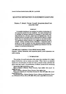
Fig.2 Empirical Q-SNR maps
According to the quantile method for low energy envelope tracking, the initial noise estimate is given by int ( qM ) 1 PˆN (l , m ) = (4) ∑ PY' (l , i ) int (qM ) + 1 i = 0 In our experiments, nominal setting are M=38 (corresponding to an approximate 600ms window) and q=0.21. Note that the window length limits the rate at which we can track non-stationary noise. 2.2. SNR estimation After the initial estimation of the noise power spectrum, the estimate of the instantaneous SNR is calculated as P (l , m ) γ (l , m ) = 10 log 10 Y (5) Pˆ (l , m ) N Note that this provides a time varying estimate of the SNR for each frequency subband. 2.3. Q-SNR map
2
S Y (l , m ) ≡ {PY (l , m − M + 1), " , PY (l , m − 1), PY (l , m )}
where M is the segment length. The data set is then sorted such that S Y' (l , m ) ≡ {PY' (l ,0), PY' (l ,1), " , PY' (l , M − 1)} where PY' (l ,0 ) ≤ PY' (l ,1) ≤ " ≤ PY' (l , M − 1)
A Q-SNR map, ψ l , is used to specify a new q value for each frequency/time point based on the initial estimated SNR. q(l , m ) = ψ l [γ (l , m )] (6) The mapping for a frequency subband is found empirically using training data corresponding to approximately 200 seconds of clean speech combined with 14 different noise types (NOISEX-92 dataset) covering an overall SNR range of –6 to 15 dB. A table is constructed by binning each estimated instantaneous (frequency/time) SNR value versus the corresponding optimal q value. The optimal q can be found by a simple line search to determine the value that subsequently yields the best estimation of the instantaneous noise level, which is known during this training phase. The mean value of q in each bin is stored as a table look-up to produce the Q-
SNR map. Note, we independently train 18 different maps corresponding to the critical frequency bands for speech. The learned Q-SNR maps are shown in Fig.2. It is observed that for SNR values below 0 dB the difference between the 18 subbands appears negligible. The interpretation of the overall shape and causes for the differences between subbands above 0 dB is still under investigation. 2.4. Second estimation
10
10
10
10
10
10
Finally, the second estimate is obtained using q(l,m) as specified by the Q-SNR maps. The computation is similar to the initial estimation, with the exception that different q values are use for each frequency/time point, int ( q (l , m ) M ) 1 ˆ (7) PˆN (l , m ) = ∑ PY' (l , i ) int (q(l , m )M ) + 1 i = 0 Note that the computation cost of this is marginal as the data set has already been sorted during the initial estimation.
10
10
10
a) Noise power estimation for a single frame
1
noise power initial est. two-pass est.
0
-1
-2
-3
0
500
1000
1500
2000
2500
3000
3500
4000
Frequency (Hz) b) Noise power estimation for a single frequency bin (l=109)
2
noise power initial est. two-pass est.
0
-2
-4
0
0.5
Time (second)
1
1.5
Fig.4 a) Noise estimation at a single time frame, b) noise estimation for frequency subband (l=109) versus time.
2.5. Performance Evaluations beginning segment initial est. two-pass est.
10
10
10
10
Noise power spectrum estimation
2
10
10
10
2
1
0
-5
0
5
10
15
SNR (db)
noisy speech noise two-pass est.
10
Averaged Relative Error
3
J
A short sentence (~ 2 seconds) with additive white noise (NOISEX-92) with SNR = 6 dB is used to illustrate performance of the two-pass quantile noise estimation algorithm. Fig.3 shows the average power spectrum for the noisy speech, noise, and the two-pass quantile noise estimation (the mean value of the instantaneous estimation is shown). The upper subplot in Fig.4 compares performance of the initial and second pass estimates for a single fixed time frame. The lower subplot compares the tracking performance for a single frequency subband (l=109) across time frames. These plots clearly show the improvement in the two-pass approach and the ability to track local variations in the noise power across time and frequency. Note that in this case we are tracking the short term statistical variations in stationary noise.
10
Fig.5 Averaged relative error versus input SNR, a) estimation is performed using the beginning segment of the waveform, b) initial quantile estimation, c) two-pass quantile estimation.
1
To provide an objective performance measure, we calculate the average relative error, ˆ PˆN (l , m ) − PN (l , m ) 1 (8) J= ∑ N fq N frm l , m PN (l , m )
0
-1
-2
0
500
1000
1500
2000
2500
3000
Frequency (Hz)
Fig.3 Noise power spectrum estimation
3500
4000
Fig.5 shows a graph of J as a function of overall input SNR level, and clearly indicates the improvement with the two-pass approach. Here the test data is 100 seconds of speech with additive car noise. Finally, Fig.6 compares histograms of instantaneous SNR estimates from which we can conclude that the two-pass approach also provides estimates which are distributed statistically more similar to the original SNR distribution.
(a)
(b) 5500
5500
5000
5000
5000
4500
4500
4500
4000
4000
4000
3500
3500
3500
3000
3000
3000
2500
2500
2500
2000
2000
2000
1500
1500
1500
1000
1000
1000
500
500
500
-50
0
50
-50
4. DISCUSSION AND CONCLUSIONS
(c)
5500
0
50
-50
0
50
SNR (db)
Fig.6 Histogram of estimated instantaneous SNR, a) actual noise spectrum, b) initial quantile estimation, c) two-pass quantile estimation.
3. APPLICATION TO SPEECH ENHANCEMENT To illustrate the performance of the two-pass quantile noise estimation in speech enhancement, we applied the algorithm to a single channel spectral subtraction based speech enhancement system using the simplified Ephraim/Malah suppression rule [5,6]. Fig.7 shows the SNR improvement as a function of input SNR level, where the test data is 100 seconds of speech with a combination of 6 different noise sources (babble, car, pink, white, factory, machinegun). The advantage of twopass algorithm is clear. Subjectively, it is observed that there is some residual noise, but very little speech distortion in the enhanced speech. The method effectively tracks slow varying non-stationary noise. However, the method does not show improvement for impulsive types of noise (e.g., clicks or machine gun noise) or for other rapidly varying noise sources such as background music. In general, the approach appears robust over a wide range of noise types providing good tradeoff between noise suppression and speech distortion. SNR improvement
8
beginning seg. initial est. two-pass est.
7
6
db
5
4
3
2
1
0 -6
-4
-2
0
2
4
6
input SNR (db)
Fig.7 SNR improvement
8
10
12
We have presented a new approach for estimating the noise spectrum given a noisy speech signal. An initial estimate is found using quantile statistics, which is then improved by performing a second estimation using the estimated SNR from the first pass. The method is capable of tracking local variation is both stationary and nonstationary noise sources. A number of extensions to this system have also been studied. These include performing additional iterative estimations as well as adding an empirical (multiplicative) correction factor after the final estimation. However, our experiments show that the performance gains are not significant enough to justify the added complexity. While we have illustrated application of the algorithm to spectral subtraction based speech enhancement, it should be noted that the algorithm can be viewed as a stand-alone component with applicability to a wide range of speech processing applications. In our group, we also use the quantile method for a wavelet-based speech enhancement method [8] as well as a Kalman Filter approach [9]. Its use for normalizing speech for ASR front-ends is also under investigation.
Acknowledgements This work was supported in part by the NSF under grant ECS-0083106 5. REFERENCES [1] Rainer Martin, “An efficient algorithm to estimate the instantaneous SNR of speech signal”, EuroSpeech’93, pp1093-1096. [2] Rainer Martin, “Spectral subtraction based on minimum statistics”, Eur. Signal Processing Conf., pp1182-1185, 1994. [3] Volker Stahl, Alexander Fischer and Rolf Bippus, “Quantile based noise estimation for spectral subtraction and wiener filtering”, ICASSP’2000, pp1875-1878. [4] Christophe Ris, Stephane Dupont, “Assessing local noise level estimation methods: application to noise robust ASR”, Speech Communication, v34, i1-2, pp141-158, Apr. 2001. [5] Patrick J. Wolfe and Simon J. Godsill, “Simple alternatives to the Ephraim and Malah suppression rule for speech enhancement”, IEEE Workshop on Statistical Signal Processing, pages 496-499, Aug. 2001. [6] O. Cappe, “Elimination of the musical noise phenomenon with the Ephraim and Malah noise suppressor”, IEEE Trans. Speech and Audio Processing, v2. n2. pp345-349, Apr. 1994. [7] H. G. Hirsch and C. Ehrlicher, “Noise estimation techniques for robust speech recognition”, ICASSP’95, pp153-156. [8] Qiang Fu and Eric A. Wan, “Perceptual speech wavelet denoising using adaptive time-frequency threshold estimation”, submitted to ICASSP’2003 [9] Eric A. Wan and Alex T. Nelson, “Removal of noise from speech using the dual EKF algorithm”, ICASSP’98, pp381384