Publications of the Astronomical Society of the Pacific, 118: 1176–1179, 2006 August 䉷 2006. The Astronomical Society of the Pacific. All rights reserved. Printed in U.S.A.
Two-Photon Transitions and Continuous Emission from Hydrogenic Species Mark C. Bottorff Department of Physics, Southwestern University, 1001 East University Avenue, Georgetown, TX 78626;
[email protected]
and Gary J. Ferland and Joseph P. Straley Department of Physics, University of Kentucky, Lexington, KY 40506;
[email protected] Received 2006 April 28; accepted 2006 June 16; published 2006 July 25
ABSTRACT. We discuss the implementation of two-photon emission and absorption in Cloudy, a generalpurpose photoionization and radiative transfer code. We now include induced two-photon absorption between the 1s and 2s levels of hydrogen and hydrogen-like ions and between the 1 1S and 2 1S levels of the He-like isoelectronic sequence. We show sample calculations predicting the full emitted continuum and have implemented a method to allow this continuum to be saved in FITS format and reused in other applications.
can take on any value between 0 and n21. In these transitions, some frequency pairs are more likely than others. Because of the symmetry of n1 and n2 about n21/2 in equation (1), this likelihood is symmetric about n21/2. Most of the effort in calculating two-photon processes goes into calculating the spontaneous two-photon transition rate (per unit frequency). Breit & Teller (1940) made the first detailed calculations of spontaneous two-photon emission rates from hydrogen and hydrogenic helium due to transitions between the 2s and 1s energy levels. Subsequent refinement was presented by Spitzer & Greenstein (1951). Brown & Mathews (1970) utilized these results to predict continuous emission from nebulae. As outlined in Spitzer & Greenstein (1951), the spontaneous two-photon transition rate is expressed as infinite sums of integrals of radial wave functions. Evaluation of these integrals is detailed in Breit & Teller (1940). In principle, approximate numerical calculation may be achieved by series truncation; however, Nussbaumer & Schmutz (1984) created a highly accurate analytical fit to the spontaneous two-photon transition rate per atom per unit relative frequency for hydrogen 2s–1s transitions, thereby eliminating the need for evaluating any sums, unless precision at a level less than fractions of a percent are required. The form and normalization of the Nussbaumer & Schmutz (1984) fit to this rate is given by
1. INTRODUCTION Here we describe the treatment of induced two-photon emission and absorption in the openly available plasma simulation code Cloudy, last reviewed by Ferland et al. (1998). This emission physics, now included with free-bound recombination continua, allows the full hydrogen continuous emission spectrum to be predicted for any density, temperature, and ionization. Rather than presenting detailed tables, we have implemented the ability to save the spectrum in FITS format for later use. 2. AN OVERVIEW OF TWO-PHOTON PROCESSES Two-photon transitions involve the simultaneous emission or absorption of two photons by an atom (or ion) and a corresponding energy-conserving change of atomic energy level. Somewhat analogous to single-photon processes, two-photon emission can be spontaneous or stimulated, whereas two-photon absorption is only stimulated. However, an important distinction is that since each photon carries one unit of angular momentum, certain transitions between atomic energy levels, forbidden for single-photon processes, are allowed in two-photon processes. Another important distinction is that the spectrum of spontaneous two-photon processes, unlike single-photon processes, is continuous. A continuous spectrum is possible because energy conservation only requires that the sum of the photon energies be equal to the energy level difference of the atom. Thus, we have n2 ⫹ n1 p n21 ,
H A2g, 2s1s, y (y)
(1)
{
(
C y(1 ⫺ y){1 ⫺ [4y(1 ⫺ y)]g} p ⫹a[y(1 ⫺ y)]b[4y(1 ⫺ y)]g for 0 ! y ! 1, 0 otherwise.
where n1 and n2 are the photon frequencies and n21 p FE 21F/h, where E21 is the energy difference between atomic energy levels 2 and 1 of the emitting (or absorbing) atom, and h is Planck’s constant. Thus, so long as equation (1) is satisfied, n1 and n2
)
(2)
1176
PHOTON TRANSITIONS IN CLOUDY 1177 H The symbolism in A2g, 2s1s, y (y) is as follows. The A is chosen to be analogous to the Einstein symbol used for spontaneous single-photon transitions. (An excellent discussion of singlephoton processes is found in Rutten [1999].) The superscript 2g denotes that this is a two-photon process, and the H superscript denotes that it is for hydrogen. The subscript 2s1s denotes the 2s–1s transition, and finally, the subscript y indicates that this expression is per unit relative frequency. To indicate that the frequency is relative to the 2s–1s transition H for hydrogen, we write y p n/n2s1s . The values of the constants on the right-hand side of equation (2) are C p 202.0 s⫺1, g p 0.8, a p 0.88, and b p 1.53. Chluba & Sunyaev (2006) used a version of this fit for cosmology-specific modeling. The total spontaneous two-photon emission rate for hydrogen, from the 2s–1s energy level, is given by
H A2g, 2s1s p
1 2
冕
1 H A2g, 2s1s, y (y)dy.
(3)
0
Since two photons correspond to one transition, a photon on H the red side of n2s1s /2 is symmetrically paired with a photon on H the blue side of n2s1s /2. Thus, the 12 is required in equation (3) to avoid double counting. One can get an estimate of how good the global fit of equation (2) is by comparing the value of H A2g, 2s1s , predicted by the fit, to contemporary detailed calculations H of A2g, 2s1s . As a simple test, we uniformly partitioned the interval y 苸 (0, 1) into 100 parts and applied the trapezoid rule to inH ⫺1 tegrate equation (2). This yields A2g, 2s1s p 8.224 s , which is within 0.05% of values obtained from detailed calculations by Goldman (1989) and Labzowsky et al. (2005). We use equation (2) in calculations presented here. Calculation of spontaneous two-photon rates per unit relative frequency per atom for hydrogen-like ions is achieved by mulH 6 tiplying A2g, 2s1s, y (y) by Z , where Z is the atomic number of the H ion ion ion, and replacing y p n/n2s1s with y p n/n2s1s , where n2s1s is the frequency of the 2s–1s transition of the ion. The rates for hydrogenic ions, placed on an absolute frequency scale, is therefore ion A2g, 2s1s, n (n) p
Z 6 2g, H ion A 2s1s, y (n/n2s1s ). ion n2s1s
(4)
ion H Of course for hydrogen itself, Z p 1 and n2s1s p n2s1s . (Note: for the remainder of this discussion, the superscript “ion” generically refers to hydrogen or hydrogen-like ions.) Once the spontaneous two-photon emission rate is calculated, the corresponding stimulated absorption and stimulated emission rates ion ⫺ n. By mireadily follow. We choose n1 p n and n2 p n2s1s croscopic time reversibility, the rate at which this single pair of photons can be absorbed (resulting in a 1s–2s transition) is equal to the spontaneous decay rate per particle per unit freion quency, A2g, 2s1s, n (n). However, in the presence of a radiation field, this rate becomes enhanced by the number of available photons in the radiation field in energy states hn1 and hn2. The number
2006 PASP, 118:1176–1179
of photons, with frequency n in a radiation field with mean intensity Jn (n), is called the photon occupation number, h(n). It is given by h(n) p Jn (n)/(2hn 3/c 2 ),
(5)
where Jn, the solid-angle–averaged intensity In(n) of the radiation field, is defined by Jn (n) p
1 4p
冕冕 2p
0
p
In (n) sin v dv df.
(6)
0
The enhanced upward transition rate (e.g., the two-photon ion absorption rate) is therefore given by A2g, 2s1s, n (n) times the product of h(n1) and h(n2). We denote the stimulated upward tran2g, ion sition rate per atom per unit frequency by B1s2s, n (n) , where we choose the symbol B to be analogous to the symbol used for stimulated single-photon emission and absorption. Substituting n1 and n2 gives 2g, ion 2g, ion ion B1s2s, n (n) p A 2s1s, n (n)h(n)h(n2s1s ⫺ n).
(7)
The reverse process, the stimulated two-photon emission rate per atom per unit frequency, is determined by similar reasoning. The only difference is that we must add 1 to each occupation number to correct for the additional photons that can be added to the radiation field from the atom. We therefore have 2g, ion 2g, ion ion B2s1s, n (n) p A 2s1s, n (n)[1 ⫹ h(n)][1 ⫹ h(n2s1s ⫺ n)].
(8)
We note that if the radiation field is a blackbody, the occupation number is h(n) p
1 . exp (hn/kT ) ⫺ 1
(9)
This, combined with detailed balance of the two-photon rates implied by the forms of equations (7) and (8), results in level populations in thermodynamic equilibrium. To demonstrate this, let n1s and n2s be the number of atoms in the 1s and 2s states, respectively. Multiplying equation (7) by n1s and equation (8) by n2s gives the rate of transitions per unit volume. By equating the rates, we obtain the asserted result; namely, ion n 2s h(n) h(n2s1s ⫺ n) p ion n1s 1 ⫹ h(n) 1 ⫹ h(n2s1s ⫺ n) ion hn h(n2s1s ⫺ n) exp ⫺ kT kT
( ) [ hn p exp (⫺ . kT ) p exp ⫺
ion 2s1s
] (10)
We implemented induced and spontaneous two-photon tran-
1178 BOTTORFF, FERLAND, & STRALEY
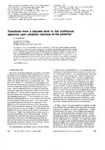
Fig. 1.—Rate per atom (s⫺1) of induced two-photon 2s–1s emission for H as a function of blackbody temperature. The gas is in the low-density limit, and the radiation is a true blackbody. The range of radiation field temperatures spans that over which hydrogen will be atomic.
sitions using the formalism described above. The full system of level balance equations is solved as in Ferland & Rees (1988). Figure 1 shows the computed rates of induced two-photon emission for the H i 2s–1s transition as a function of temperature. In the calculations in this figure, a low-density gas (nH p 1 cm⫺3) is exposed to a true blackbody radiation field with various temperatures. The range of temperatures spans those in which atomic hydrogen is present. The vertical axis shows the induced rate (eq. [8]) integrated over frequency. Note that the rate is always smaller than the spontaneous rate. We found that two-photon stimulated emission and absorption are never very important for irradiation by a thermal continuum. The reason is shown by inspection of equation (8). The process is only important when the photon occupation numbers are significantly greater than unity at the ultraviolet wavelengths that affect the 2s–1s transition. This is an intense radiation field, which, for any reasonable continuum shape, will ionize hydrogen, and so little H0 will be present. The process will be most important when H0 is present near intense infrared continua. This is the case, for instance, considered by Chluba & Sunyaev (2006). Irradiation by a nonthermal continuum, such as that found in an active galactic nucleus, is another example. Tests show that for broad-line region clouds within the grids computed by Korista et al. (1997), those with a flux of hydrogen-ionizing photons greater than f(H) ≈ 10 22 cm⫺2 s⫺1 have induced two-photon rates that are faster than the spontaneous rates. The result is that the process alters the populations of the n p 2 levels of H0. We conclude that the process must be included for completeness in numerical simulations of highly nonthermal environments.
Fig. 2.—Emission (ergs cm3 s⫺1) vs. wavelength (mm) from an optically thin hydrogen gas at various densities and a temperature of 104 K. From the thinnest line to the thickest line, the densities are respectively 1, 102, 104, and 106 cm⫺3. (Note: The plots corresponding to the two lowest densities completely overlap at the resolution of the graph.)
3. EXAMPLE CONTINUA We show some sample hydrogen recombination continua in Figures 2 and 3. These are the result of the solution of the full set of capture-cascade recombination equations for hydrogen (Osterbrock & Ferland 2006, hereafter AGN3), with recombination emission predicted from the photoionization cross sections using the Milne relation (AGN3). Further details are given in Ferland & Rees (1988) and Ferguson & Ferland (1997). The figures show the emission from an optically thin cell of gas divided by the product of the electron and proton number density. In both figures, the vertical axis is 4pn jn (T )/ne n p in units of ergs cm3 s⫺1, where jn (T ) is the volume emissivity (ergs s⫺1
Fig. 3.—Emission (ergs cm3 s⫺1) vs. wavelength (mm) from an optically thin hydrogen gas at various temperatures. From the thinnest line to the thickest line, the temperatures are 5000, 10,000, 15,000, and 20,000 K, respectively.
2006 PASP, 118:1176–1179
PHOTON TRANSITIONS IN CLOUDY 1179 cm⫺3), and the horizontal axis is wavelength in mm. The figures show a small part of the full continuum computed by Cloudy. The actual calculation covers the much larger continuum range, from 100 MeV to 8.66 m. Figure 2 shows the emission for a range of densities at a constant temperature of 104 K. From the thinnest line to the thickest line, the densities are respectively 1, 102, 104, and 106 cm⫺3. (Note: In Fig. 2, the lines corresponding to the two lowest densities completely overlap at the resolution of the graph.) The free-bound recombination edges are the strong abrupt features that are present, starting with the Lyman continuum at 0.0912 mm and extending through the Balmer, Paschen, etc., continua. Figure 3 shows a similar plot for a range of temperatures at a density of 1 cm⫺3. This is safely in the lowdensity limit. From the thinnest line to the thickest line, the temperatures are 5000, 10,000, 15,000, and 20,000 K, respectively. The stimulated two-photon continuum contribution is prominent in both figures, peaking shortward of the spontaneous two-photon peak (∼0.24 mm). This result is consistent with the results of Gaskell (1980), who obtained a peak of 0.162 mm for two-photon rates applied from quasar emission-line clouds. In Figure 2, it is strong for the three lowest densities, but is collisionally suppressed at higher densities (AGN3). In Figure 2, apparent changes in the two-photon continuum are actually due to changes in the underlying Balmer continuum— the shape of the two-photon continuum has no temperature dependence. It is obvious that a broad range of spectra can result. Similar calculations are presented in Ferland (1980), although these did not include two-photon emission. Previous studies have presented such curves as tables, which are then used for interpolation. It is possible to do better with today’s machines. We have added to Cloudy the ability to output predicted continua in FITS format (Porter et al. 2006). It is then
easy to generate a full continuum for any density, temperature, and composition, with a quick calculation. A sample input script as follows: // the log of the hydrogen density hden 5.4 // we want a pure hydrogen gas init “honly.ini” // the assumed kinetic temperature in K constant temperature 10,000 K // predict emission from a unit volume // log thickness in cm set dr 0 // save the file punch diffuse continuum FITS “test.con” This allows the continuous emission to be computed for any physical conditions, saved as a standard FITS file, and then reused in any other application that can handle the FITS format.
4. SUMMARY We have outlined the treatment of induced two-photon processes in Cloudy. It is doubtful that the process dominates in any astrophysical environment involving irradiation by a thermal source, such as a star. This is because the intense radiation field that is required to produce significant rates will also ionize the atom or ion for a thermal continuum. The induced twophoton rates can be much faster than the spontaneous rates when the gas is irradiated by a highly nonthermal spectrum, such as that found in an active nucleus. We have shown examples of the full computed hydrogen emission spectrum at a variety of densities and temperatures and have outlined a facility to obtain such spectra by using Cloudy.
REFERENCES Breit, G., & Teller, E. 1940, ApJ, 91, 215 Brown, R. L., & Mathews, W. G. 1970, ApJ, 160, 939 Chluba, J., & Sunyaev, R. A. 2006, A&A, 446, 39 Ferguson, J. W., & Ferland, G. J. 1997, ApJ, 479, 363 Ferland, G. J. 1980, PASP, 92, 596 Ferland, G. J., Korista, K. T., Verner, D. A., Ferguson, J. W., Kingdon, J. B., & Verner, E. M. 1998, PASP, 110, 761 Ferland, G. J., & Rees, M. J. 1988, ApJ, 332, 141 Gaskell, C. M. 1980, Observatory, 100, 148 Goldman, S. P. 1989, Phys. Rev. A, 40, 1185 Korista, K. T., Baldwin, J. A., & Ferland, G. J., & Verner, D. 1997, ApJS, 108, 401
2006 PASP, 118:1176–1179
Labzowsky, L. N., Shonin, A. V., & Solovyev, D. A. 2005, J. Phys. B, 38, 265 Nussbaumer, H., & Schmutz, W. 1984, A&A, 138, 495 Osterbrock, D. E., & Ferland, G. J. 2006, Astrophysics of Gaseous Nebulae and Active Galactic Nuclei (2nd ed.; Sausalito: University Science Books) (AGN3) Porter, R., Ferland, G., Kraemer, S., Armentrout, B., Arnaud, K., & Turner, T. J. 2006, PASP, 118, 920 Rutten, R. J. 1999, Radiative Transfer in Stellar Atmospheres (Utrecht: Sterrekundig Inst.), 53 Spitzer, L., & Greenstein, J. L. 1951, ApJ, 114, 407