Two simple full-text indexes based on the suffix array

Two simple full-text indexes based on the suffix array Szymon Grabowski and Marcin Raniszewski

arXiv:1405.5919v1 [cs.DS] 22 May 2014

Lodz University of Technology, Institute of Applied Computer Science, Al. Politechniki 11, 90–924 L´ od´z, Poland {sgrabow|mranisz}@kis.p.lodz.pl

Abstract. We propose two suffix array inspired full-text indexes. One, called SA-hash, augments the suffix array with a hash table to speed up pattern searches due to significantly narrowed search interval before the binary search phase. The other, called FBCSA, is a compact data structure, similar to M¨ akinen’s compact suffix array, but working on fixed sized blocks, which allows to arrange the data in multiples of 32 bits, beneficial for CPU access. Experimental results on the Pizza & Chili 200 MB datasets show that SA-hash is about 2.5–3 times faster in pattern searches (counts) than the standard suffix array, for the price of requiring 0.3n − 2.0n extra space, where n is the text length, and setting a minimum pattern length. The latter limitation can be removed for the price of even more extra space. FBCSA is relatively fast in single cell accesses (a few times faster than related indexes at about the same or better compression), but not competitive if many consecutive cells are to be extracted. Still, for the task of extracting e.g. 10 successive cells its time-space relation remains attractive. Keywords: suffix array, compressed indexes, compact indexes, hashing

1

Introduction

The field of text-oriented data structures continues to bloom. Curiously, in many cases several years after ingenious theoretical solutions their more practical (which means: faster and/or simpler) counterparts are presented, to mention only recent advances in rank/select implementations [11] or the FM-index reaching the compression ratio bounded by k-th order entropy with very simple means [17]. Despite the great interest in compact or compressed1 full-text indexes in recent years [22], we believe that in some applications search speed is more important than memory savings, thus different space-time tradeoffs are worth being explored. The classic suffix array (SA) [21], combining speed, simplicity and often reasonable memory use, may be a good starting point for such research. In this paper we present two SA-based full-text indexes, combining effectiveness and simplicity. One is augments the standard SA with a hash table to speed up searches, for a moderate overhead in the memory use, the other is a byte-aligned variant of M¨akinen’s compact suffix array [19,20].

2

Preliminaries

We use 0-based sequence notation, that is, a sequence S of length n is written as S[0 . . . n − 1], or equivalently as s0 s1 . . . sn−1 . 1

By the latter we mean indexes with space use bounded by O(nH0 ) or even O(nHk ) bits, where n is the text length, σ the alphabet size, and H0 and Hk respectively the order-0 and the order-k entropy. The former term, compact full-text indexes, is less definite, and, roughly speaking, may fit any structure with less than n log2 n bits of space, at least for “typical” texts.

One may define a full-text index over text T of length n as a data structure supporting (at least) two basic types of queries, both with respect to a pattern P of length m, both T and P over a common finite integer alphabet of size σ. One query type is count: return the number occ ≥ 0 of occurrences of P in T . The other query type is locate: for each pattern occurrence report its position in T , that is, such j that P [0 . . . m − 1] = T [j . . . j + m − 1]. The suffix array SA[0 . . . n − 1] for text T is a permutation of the indexes {0, 1, . . . , n−1} such that T [SA[i] . . . n−1] ≺ T [SA[i+1] . . . n−1] for all 0 ≤ i < n−1, where the “≺” relation is the lexicographical order. The inverse suffix array SA−1 is the inverse permutation of SA, that is, SA−1 [j] = i ⇔ SA[i] = j. If not stated otherwise, all logarithms throughout the paper are in base 2.

3

Related work

The full-text indexing history starts with the suffix tree (ST) [25], a trie whose string collection is the set of all the suffixes of a given text, with an additional requirement that all non-branching paths of edges are converted into single edges. Typically, each ST path is truncated as soon as it points to a unique suffix. A leaf in the suffix tree holds a pointer to the text location where the corresponding suffix starts. As there are n leaves, no non-branching nodes and edge labels represented with pointers to the text, the suffix tree takes O(n) words of space, which is in turn O(n log n) bits. The structure can be built in linear time (e.g., [25,3]). Moreover, the linear-time construction algorithms can be fast not only in theory, but also in practice [14]. Assuming constant-time access to any child of a given node, the search in the ST takes only O(m + occ) time in the worst case. In practice, this is cumbersome for a large alphabet (requires using perfect hashing, which also makes the construction time linear only in expectation). A small alphabet is easier to handle, which goes in line with the wide use of the suffix tree in bioinformatics. The main problem with the suffix tree are its large space requirements, even in the most economical version [18] reaching almost 9n bytes on average (and 16n in the worst case), plus the text, for σ ≤ 256, and even more for large alphabets. Most implementations need 20n or more space. An important alternative to the suffix tree is the suffix array (SA) [21]. It is an array of n pointers to text suffixes arranged in the order of lexicographic ordering of the sequences (i.e., the suffixes) the pointers store references to. The SA needs n log n bits for its n suffix pointers (indexes), plus n log σ bits for the text, which typically translates to 5n bytes in total. The pattern search time is O(m log n) in the worst case and O(m logσ n + log n) on average, which can be improved to O(m + log n) in the worst case using the longest common prefix (lcp) table. Alternatively, the O(m+log n) time can be reached even without the lcp, in a more theoretical solution with a specific suffix permutation [8]. Yet Manber and Myers in their seminal paper [21] presented a nice trick saving several first steps in the binary search: if we know the SA intervals for all the possible first k symbols of the pattern, we can immediately start the binary search in a corresponding interval. We can set k close to logσ n, with O(n log n) extra bits of space, but constant expected size of the interval, which leads to O(m) average search time and only O(m/|cache line|) cache misses on average, where |cache line| is the cache line length expressed in symbols (typically 64 symbols / bytes in a modern 2

CPU). Unfortunately, real texts are far from random, hence in practice, if text symbols are bytes, we can use k up to 3, which offers a limited (yet, non-negligible) benefit. This idea, later denoted as using a lookup table (LUT), is fairly well known, see e.g. its impact in the search over a suffix array on words [4]. A number of suffix tree or suffix array inspired indexes have been proposed as well, including the suffix cactus [16] and the enhanced suffix array (ESA) [1], with space use usually between SA and ST, but according to our knowledge they generally are not faster than their famous predecessors in the count or locate queries. On a theoretical front, the suffix tray by Cole et al. [2] allows to achieve O(m + log σ) search time (with O(n) worst-case time construction and O(n log n) bits of space), which was recently improved by Fischer and Gawrychowski [7] to O(m + log log σ) deterministic time, with preserved construction cost complexities. The common wisdom about the practical performance of ST and SA is that they are comparable, but Grimsmo in his interesting experimental work [14] showed that a careful ST implementation may be up to about 50% faster than SA if the number of matches is very small (in particular, one hit), but if the number of hits grows, the SA becomes more competitive, sometimes being even about an order of magnitude faster. Another conclusion from Grimsmo’s experiments is that the ESA may also be moderately faster than SA if the alphabet is small (say, up to 8) but SA easily wins for a large alphabet. Since around 2000 we can witness a great interest in succinct data structures, in particular, text indexes. Two main ideas that deserve being mentioned are the compressed suffix array (CSA) [15,24] and the FM-index [6]; the reader is referred to the survey [22] for an extensive coverage of the area. It was noticed in extensive experimental comparisons [5,11] that compressed indexes are not much slower (and sometimes comparable) to the suffix array in count queries, but locate is 2–3 orders of magnitude slower if the number of matches is large. This instigated researchers to follow one of two paths in order to mitigate the locate cost for succinct indexes. One, pioneered by M¨akinen [19,20] and addressed in a different way by Gonz´alez et al. [12,13], exploits repetitions in the suffix array (the idea is explained in Section 5). The other approach is to build semi-external data structures (see [9,10] and references therein).

4

Suffix Array with Deep Buckets

The mentioned idea of Manber and Myers with precomputed interval (bucket) boundaries for k starting symbols tends to bring more gain with growing k, but also precomputing costs grow exponentially. Obviously, σ k integers are needed to be kept in the lookup table. Our proposal is to apply hashing on relatively long strings, with an extra trick to reduce the number of collisions. We start with building the hash table HT (Fig. 1). The hash function is calculated for the distinct k-symbol (k ≥ 2) prefixes of suffixes from the (previously built) suffix array. That is, we process the suffixes in their SA order and if the current suffix shares its k-long prefix with its predecessor, it is skipped (line 8). The value written to HT (line 11) is a pair: (the position in the SA of the first suffix with the given prefix, the position in the SA of the last suffix with the given prefix). Linear probing 3

is used as the collision resolution method. As for the hash function, we used sdbm (http://www.cse.yorku.ca/~ oz/hash.html). Fig. 2 presents the pattern search (locate) procedure. It is assumed that the pattern length m is not less than k. First the range of rows in the suffix array corresponding to the first two symbols of the pattern is found in a “standard” lookup table (line 1); an empty range immediately terminates the search with no matches returned (line 2). Then, the hash function over the pattern prefix is calculated and a scan over the hash table performed until no extra collisions (line 5; return no matches) or found a match over the pattern prefix, which give us information about the range of suffixes starting with the current prefix (line 6). In this case, the binary search strategy is applied to narrow down the SA interval to contain exactly the suffixes starting with the whole pattern. (As an implementation note: the binary search could be modified to ignore the first k symbols in the comparisons, but it did not help in our experiments, due to specifics of the used A strcmp function from the asmlib library2 ). HT build(T [0 . . . n − 1], SA[0 . . . n − 1], k, z, h(.)) Precondition: k ≥ 2 (1) allocate HT [0 . . . z − 1] (2) for j ← 0 to z − 1 do HT [j] ← N IL (3) prevStr ← ε (4) j ← N IL (5) lef t ← N IL; right ← N IL (6) for i ← 0 to n − 1 do (7) if SA[i] ≥ n − k then continue (8) if T [SA[i] . . . SA[i] + k − 1] 6= prevStr then (9) if j 6= N IL then (10) right ← i − 1 (11) HT [j] ← (lef t, right) (12) j ← h(T [SA[i] . . . SA[i] + k − 1]) (13) prevStr ← T [SA[i] . . . SA[i] + k − 1] (14) repeat (15) if HT [j] = N IL then (16) lef t ← i (17) break (18) else j ← (j + 1) % z (19) until false (20) HT [j] ← (right + 1, n − 1) (21) return HT

Figure 1. Building the hash table of a given size z

5

Fixed Block based Compact Suffix Array

We propose a variant of M¨akinen’s compact suffix array [19,20], whose key feature is finding repeating suffix areas of fixed size (e.g., 32). This allows to maintain a byte aligned data layout, beneficial for speed and simplicity. Even more, by setting a (natural) restriction on one of the key parameters we force the structure’s building bricks to be multiples of 32 bits, which prevents misaligned access to data. 2

http://www.agner.org/optimize/asmlib.zip, v2.34, by Agner Fog.

4

Pattern search(T [0 . . . n − 1], SA[0 . . . n − 1], HT [0 . . . z − 1], k, h(.), P [0 . . . m − 1]) Precondition: m ≥ k ≥ 2 (1) (2) (3) (4) (5) (6) (7) (8) (9)

beg, end ← LU T2 [p0 , p1 ] if end < beg then report no matches; return j ← h(P [0 . . . k − 1]) repeat if HT [j] = N IL then report no matches; return if (beg ≤ HT [j].lef t ≤ end) and (T [SA[HT [j]] . . . SA[HT [j]] + k − 1] = P [0 . . . k − 1]) then binSearch(P [0 . . . m − 1], HT [j].lef t, HT [j].right); return j ← (j + 1) % z until false

Figure 2. Pattern search

M¨akinen’s index was the first opportunistic scheme for compressing a suffix array, that is such that uses less space on compressible texts. The key idea was to exploit runs in the SA, that is, maximal segments SA[i . . . i + ℓ − 1] for which there exists another segment SA[j . . . j +ℓ−1], such that SA[j +s] = SA[i+s]+1 for all 0 ≤ s < ℓ. This structure still allows for binary search, only the accesses to SA cells require local decompression. We resign from maximal segments in our proposal. The construction algorithm for our structure, called fixed block based compact suffix array (FBCSA), is presented in Fig. 3. As a result, we obtain two arrays, arr1 and arr2 , which are empty at the beginning, and their elements are always appended at the end during the construction. The elements appended to arr1 are single bits or pairs of bits while arr2 stores suffix array indexes (32-bit integers). The construction makes use of the suffix array SA of text T , the inverse suffix array SA−1 and T BW T (which can be obtained from T and SA, that is, T BW T [i] = T [(SA[i] − 1) mod n]). Additionally, there are two construction-time parameters: block size bs and sampling step ss. The block size tells how many successive SA indexes are encoded together and is assumed to be a multiple of 32, for int32-alignment of the structure layout. The parameter ss means that every ss-th SA index will be represented verbatim. This sampling parameter is a time-space tradeoff; using larger ss reduces the overall space but decoding a particular SA index typically involves more recursive invocations. Let us describe the encoding procedure for one block, SA[j . . . j + bs − 1], where j is a multiple of bs. First we find the three most frequent symbols in T BW T [j . . . j + bs − 1] and store them (in arbitrary order) in a small helper array MF S[0 . . . 2] (line 4). If the current block of T BW T does not contain three different symbols, the NIL value will be written in the last one or two cell(s) of MF S. Then we write information about the symbols from MF S in the current block of T BW T into arr1 : we append 2-bit combination (00, 01 or 10) if a given symbol is from MF S and the remaining combination (11) otherwise (lines 5–9). We also store the positions of the first occurrences of the symbols from MF S in the current block of T BW T , using the variables pos0 , pos1 , pos2 (lines 10– 12); again NIL values are used if needed. These positions allow to use links to runs 5

of suffixes preceding subsets of the current ones marked by the respective symbols from MF S. We believe that a small example will be useful here. Let bs = 8 and the current block be SA[400 . . . 407] (note this is a toy example and in the real implementation bs must be a multiple of 32). The SA block contains the indexes: 1000, 522, 801, 303, 906, 477, 52, 610. Let their preceding symbols (from T BW T ) be: a, b, a, c, d, d, b, b. The three most frequent symbols, written to MF S, are thus: b, a, d. The first occurrences of these symbols are at positions: 401, 400 and 404, respectively (that is, 400 + pos0 = 401, etc.). The SA offsets: 521 (= 522 − 1), 999 (= 1000 − 1) and 905 (= 906 − 1) will be linked to the current block. We conclude that the preceding groups of suffix offsets are: [521, 522, 523] (as there are three symbols b in the current block of T BW T ), [999, 1000] and [905, 906]. We come back to the pseudocode. The described (up to three) links are obtained thanks to SA−1 (lines 14–16) and are written to arr2 . Finally, the offsets of the suffixes preceded with a symbol not from MF S (if any) have to be written to arr2 explicitly. Additionally, the sampled suffixes (i.e., those whose offset modulo ss is 0) are handled in the same way (line 18). To distinguish between referrentially encoded and explicitly written suffix offsets, we spent a bit per suffix and append them to arr1 (lines 19–20). To allow for easy synchronization between the portions of data in arr1 and arr2 , the size of arr2 (in bytes) as it was before processing the current block is written to arr1 (line 21).

6

Experimental Results

All experiments were run on a laptop computer with an Intel i3 2.1 GHz CPU, equipped with 8 GB of DDR3 RAM and running Windows 7 Home Premium SP1 64-bit. All codes were written in C++ and compiled with Microsoft Visual Studio 2010. The source codes for the FBCSA algorithm can be downloaded from http://ranisz.iis.p.lodz.pl/indexes/fbcsa/. The test datasets were taken from the popular Pizza & Chili site (http://pizzachili.dcc.uchile.cl/). We used the 200-megabyte versions of the files dna, english, proteins, sources and xml. In order to test the search algorithms, we generated 500 thousand patterns for each used pattern length; the patterns were extracted randomly from the corresponding datasets (i.e., each pattern returns at least one match). In the first experiment we compared pattern search (count) speed using the following indexes: plain suffix array (SA), suffix array with a lookup table over the first 2 symbols (SA-LUT2), suffix array with a lookup table over the first 3 symbols (SA-LUT3), the proposed suffix array with deep buckets, with hashing the prefixes of length k = 8 (only for dna k = 12 and for proteins k = 5 is used); the load factor α in the hash table was set to 50% (SA-hash), – the proposed fixed block based compact suffix array with parameters bs = 32 and ss = 5 (FBCSA), – FBCSA (parameters as before) with a lookup table over the first 2 symbols (FBCSA-LUT2), – – – –

6

FBCSA build(SA[0 . . . n − 1], T BW T , bs, ss) /* assume n is a multiple of bs */ (1) arr1 ← [ ]; arr2 ← [ ] (2) j ← 0 (3) repeat /* current block of the suffix array is SA[j . . . j + bs − 1] */ (4) find 3 most frequent symbols in T BW T [j . . . j + bs − 1] and store them in M F S[0 . . . 2] /* if there are less than 3 distinct symbols in T BW T [j . . . j + bs − 1], the trailing cells of M F S[0 . . . 2] are set to N IL) */ (5) for i ← 0 to bs − 1 do (6) if T BW T [j + i] = M F S[0] then arr1 .append(00) (7) else if T BW T [j + i] = M F S[1] then arr1 .append(01) (8) else if T BW T [j + i] = M F S[2] then arr1 .append(10) (9) else arr1 .append(11) (10) pos0 = T BW T [j . . . j + bs − 1].pos(M F S[0]) (11) pos1 = T BW T [j . . . j + bs − 1].pos(M F S[1]) /* set N IL if M F S[1] = N IL */ (12) pos2 = T BW T [j . . . j + bs − 1].pos(M F S[2]) /* set N IL if M F S[2] = N IL */ (13) a2s = |arr2 | (14) arr2 .append(SA−1 [SA[j + pos0 ] − 1]) (15) arr2 .append(SA−1 [SA[j + pos1 ] − 1]) /* append −1 if pos1 = N IL */ (16) arr2 .append(SA−1 [SA[j + pos2 ] − 1]) /* append −1 if pos2 = N IL */ (17) for i ← 0 to bs − 1 do (18) if (T BW T [j + i] 6∈ {M F S[0], M F S[1], M F S[2]}) or (SA[j + i] % ss = 0) then (19) arr1 .append(1); arr2 .append(SA[j + i]) (20) else arr1 .append(0) (21) arr1 .append(a2s) (22) j ← j + bs (23) if j = n then break (24) until false (25) return (arr1 , arr2 )

Figure 3. Building the fixed block based compact suffix array (FBCSA)

7

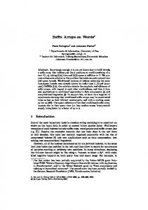
– FBCSA (parameters as before) with a lookup table over the first 3 symbols (FBCSA-LUT3), – FBCSA (parameters as before) with a hashes of prefixes of length k = 8 (only for dna k = 12 and for proteins k = 5 is used); the load factor in the hash table was set to 50% (FBCSA-hash). The results are presented in Fig. 4. As expected, SA-hash is the fastest index among the tested ones. The reader may also look at Table 1 with a rundown of the achieved speedups, where the plain suffix array is the baseline index and its speed is denoted with 1.00. m = 16 SA SA-LUT2 SA-LUT3 SA-hash m = 64 SA SA-LUT2 SA-LUT3 SA-hash

dna

english

proteins

sources

xml

1.00 1.13 1.17 3.75

1.00 1.34 1.49 2.88

1.00 1.36 1.61 2.70

1.00 1.43 1.65 2.90

1.00 1.35 1.47 2.03

1.00 1.12 1.17 3.81

1.00 1.33 1.49 2.87

1.00 1.34 1.58 2.62

1.00 1.42 1.64 2.75

1.00 1.34 1.44 1.79

Table 1. Speedups with regard to the search speed of the plain suffix array, for the five datasets and pattern lengths m = 16 and m = 64

The SA-hash index has two drawbacks: it requires significantly more space than the standard SA and we assume (at construction time) a minimal pattern length mmin . The latter issue may be eliminated, but for the price of even more space use; namely, we can build one hash table for each pattern length from 1 to mmin (counting queries for those short patterns do not ever need to perform binary search over the suffix array). For the shortest lengths ({1, 2} or {1, 2, 3}) lookup tables may be alternatively used. We have not implemented this “all-HT” variant, but it is easy to estimate the memory use for each dataset. To this end, one needs to know the number of distinct q-grams for q ≤ mmin (Table 2). q 1 2 3 4 5 6 7 8 9 10

dna 16 152 683 2,222 5,892 12,804 28,473 80,397 279,680 1,065,613

english 225 10,829 102,666 589,230 2,150,525 5,566,993 11,599,445 20,782,043 33,143,032 48,061,001

proteins 25 607 11,607 224,132 3,623,281 36,525,895 94,488,651 112,880,347 117,199,335 119,518,691

sources 230 9,525 253,831 1,719,387 5,252,826 10,669,627 17,826,241 26,325,724 35,666,486 45,354,280

xml 96 7,054 141,783 908,131 2,716,438 5,555,190 8,957,209 12,534,152 16,212,609 20,018,262

Table 2. The number of distinct q-grams (1 . . . 10) in the datasets. The number of distinct 12-grams for dna is 13,752,341.

The number of bytes for one hash table with z entries and 0 < α ≤ 1 load factor is, in our implementation, z ×8 ×(1/α), since each entry contains two 4-byte integers. 8

dna.200MB

60

40 30 20 10 10

20

30

m

40

50

20

40

10

20

30

m

40

50

SA-hash FBCSA-hash SA FBCSA SA-LUT2 FBCSA-LUT2 SA-LUT3 FBCSA-LUT3

50

30 20 10

60

sources.200MB

60

SA-hash FBCSA-hash SA FBCSA SA-LUT2 FBCSA-LUT2 SA-LUT3 FBCSA-LUT3

50 search time / pattern (us)

30

0

60

proteins.200MB

60

0

40

10

search time / pattern (us)

0

SA-hash FBCSA-hash SA FBCSA SA-LUT2 FBCSA-LUT2 SA-LUT3 FBCSA-LUT3

50 search time / pattern (us)

search time / pattern (us)

50

english.200MB

60

SA-hash FBCSA-hash SA FBCSA SA-LUT2 FBCSA-LUT2 SA-LUT3 FBCSA-LUT3

40 30 20 10

10

20

30

m

40

50

0

60

10

20

m

40

50

60

xml.200MB

60

SA-hash FBCSA-hash SA FBCSA SA-LUT2 FBCSA-LUT2 SA-LUT3 FBCSA-LUT3

50 search time / pattern (us)

30

40 30 20 10 0

10

20

30

m

40

50

60

Figure 4. Pattern search time (count query). All times are averages over 500K random patterns of the same length m = {mmin , 16, 32, 64}, where mmin is 8 for most datasets except for dna (12) and proteins (5). The patterns were extracted from the respective texts.

9

For example, in our experiments the hash table for english needed 20,782,043 ×16 = 332,512,688 bytes, i.e., 158.6% of the size of the text itself. An obvious idea to reduce the HT space, in an open addressing scheme, is increasing its load factor α. The search times then are, however, likely to grow. We checked several values of α on two datasets (Table 3) to conclude that using α = 80% may be a reasonable alternative to α = 50%, as the pattern search times grow by only about 10%.

dna, m = 12 dna, m = 16 dna, m = 32 dna, m = 64 english, m = 8 english, m = 16 english, m = 32 english, m = 64

25 1.088 1.359 1.320 1.345 1.292 1.670 1.665 1.714

50 1.111 1.362 1.347 1.394 1.386 1.761 1.762 1.794

HT load factor (%) 60 70 1.122 1.172 1.389 1.421 1.360 1.391 1.409 1.428 1.402 1.487 1.781 1.846 1.813 1.858 1.829 1.869

80 1.214 1.491 1.463 1.491 1.524 1.892 1.931 1.967

90 1.390 1.668 1.662 1.672 1.617 1.998 2.015 2.039

Table 3. Average pattern search times (in µs) in function of the HT load factor α for the SA-hash algorithm

Finally, in Table 4 we present the overall space use for the four non-compact SA variants: plain SA, SA-LUT2, SA-LUT3 and SA-hash, plus SA-allHT, which is a (not implemented) structure comprising a suffix array, a LUT2 and one hash table for each k ∈ {3, 4, . . . , mmin }. The space is expressed as a multiple of the text length n (including the text), which is for example 5.000 for the plain suffix array. We note that the lookup table structures become a relatively smaller fraction when larger texts are indexed. For the variants with hash tables we take two load factors: 50% and 80%. SA SA-LUT2 SA-LUT3 SA-hash-50 SA-hash-80 SA-allHT-50 SA-allHT-80

dna 5.000 5.001 5.321 6.050 5.657 6.472 5.920

english 5.000 5.001 5.321 6.587 5.992 8.114 6.947

proteins 5.000 5.001 5.321 5.278 5.174 5.296 5.185

sources 5.000 5.001 5.321 7.010 6.257 9.736 7.960

xml 5.000 5.001 5.321 5.958 5.600 7.353 6.471

Table 4. Space use for the non-compact data structures as a multiple of the indexed text size (including the text). The value of mmin for SA-hash-50 and SA-hash-80, used in the construction of these structures and affecting their size, is like in the experiments from Fig. 4. The index SA-allHT-* contains one hash table for each k ∈ {3, 4, . . . , mmin }, when mmin depends on the current dataset, as explained. The -50 and -80 suffixes in the structure names denote the hash load factors (in percent).

In the next set of experiments we evaluated the FBCSA index. Its properties of interest, for various block size (bs) and sampling step (ss) parameters, are: the space use, pattern search times, times to access (extract) one random SA cell, times to access (extract) multiple consecutive SA cells. For bs we set the values 32 and 64. The ss was tested in a wider range (3, 5, 8, 16, 32). Using bs = 64 results in better compression but decoding a cell is also slightly slower (see Fig. 5). Unfortunately, our tests were run under Windows and it was not easy for us to adapt other competitive compact indexes to run on our platform, yet from the comparison with the results presented 10

FBSA, compression (bs = 32)

3.0 2.5 2.0 1.5 1.0 0

3.0 2.5 2.0 1.5

5

10

15

ss

20

25

30

1.0 0

35

FBSA, access time to 1 random cell (bs = 32)

2.0

3.0 2.5 access time per cell (us)

access time per cell (us)

2.5

5

10

15

ss

20

25

30

35

FBSA, access time to 1 random cell (bs = 64)

dna english proteins sources xml

3.0

dna english proteins sources xml

3.5

index size / text size

3.5

index size / text size

FBSA, compression (bs = 64)

dna english proteins sources xml

1.5 1.0 0.5

2.0

dna english proteins sources xml

1.5 1.0 0.5

0.0 0

5

10

15

ss

20

25

30

35

0.0 0

5

10

15

ss

20

25

30

35

Figure 5. FBCSA index sizes and cell access times with varying ss parameter (3, 5, 8, 16, 32). The parameter bs was set to 32 (left figures) or 64 (right figures). The times are averages over 10M random cell accesses.

in [13, Sect. 4] we conclude that FBCSA is a few times faster in single cell access than the other related algorithms, MakCSA [20] (augmented with a compressed bitmap from [23] to extract arbitrary ranges of the suffix array) and LCSA / LCSA-Psi [13], at similar or better compression. Extracting c consecutive cells is not however an efficient operation for FBCSA (as opposed to MakCSA and LCSA / LCSA-Psi, see Figs 5–7 in [13]), yet for small ss the time growth is slower than linear, due to a few sampled (and thus written explicitly) SA offsets in a typical block (Fig. 6). Therefore, in extracting (only) 5 or 10 successive cells our index is still competitive.

7

Conclusions

We presented two simple full-text indexes. One, called SA-hash, speeds up standard suffix array searches with reducing significantly the initial search range, thanks to a hash table storing range boundaries of all intervals sharing a prefix of a specified length. Despite its simplicity, we are not aware of such use of hashing in exact pattern matching, and the approximately 3-fold speedups compared to a standard SA may be worth the extra space in many applications. The other presented data structure is a compact variant of the suffix array, related to M¨akinen’s compact SA [20]. Our solution works on blocks of fixed size, which provides int32 alignment of the layout. This index is rather fast in single cell access, but not competitive if many (e.g., 100) consecutive cells are to be extracted. 11

8

time per query (us)

7 6

FBSA (bs = 32), extracting 5 consecutive cells

10

dna english proteins sources xml

9 8 time per query (us)

9

5 4 3

14

time per query (us)

12 10

6 5 4

2 5

10

15

ss

20

25

30

10

35

FBSA (bs = 32), extracting 10 consecutive cells

18

dna english proteins sources xml

16 14 time per query (us)

16

8 6

12

2

4 10

15

ss

20

25

30

35

10

15

ss

20

25

30

35

FBSA (bs = 64), extracting 10 consecutive cells

dna english proteins sources xml

8 6

5

5

10

4

00

dna english proteins sources xml

3

2 10

7

FBSA (bs = 64), extracting 5 consecutive cells

20

5

10

15

ss

20

25

30

35

Figure 6. FBCSA, extraction time for c = 5 (top figures) and c = 10 (bottom figures) consecutive cells, with varying ss parameter (3, 5, 8, 16, 32). The parameter bs was set to 32 (left figures) or 64 (right figures). The times are averages over 1M random cell run extractions.

12

Several aspects of the presented indexes requires further study. In the SA-hash scheme collisions in the HT may be eliminated with using perfect hashing or cuckoo hashing. This should also reduce the overall space use. In case of plain text, the standard suffix array component may be replaced with a suffix array on words [4], with possibly new interesting space-time tradeoffs. The idea of deep buckets may be incorporated into some compressed indexes, e.g., to save on the several first LFmapping steps in the FM-index.

Acknowledgement The work was supported by the Polish Ministry of Science and Higher Education under the project DEC-2013/09/B/ST6/03117 (both authors).

References 1. 2. 3. 4. 5. 6. 7. 8. 9. 10.

11. 12. 13. 14.

15.

16. 17.

18.

19.

M. I. Abouelhoda, S. Kurtz, and E. Ohlebusch: The enhanced suffix array and its applications to genome analysis, in Algorithms in Bioinformatics, Springer, 2002, pp. 449–463. R. Cole, T. Kopelowitz, and M. Lewenstein: Suffix trays and suffix trists: structures for faster text indexing, in Automata, Languages and Programming, Springer, 2006, pp. 358–369. M. Farach: Optimal suffix tree construction with large alphabets, in Proceedings of the 38th IEEE Annual Symposium on Foundations of Computer Science, 1997, pp. 137–143. P. Ferragina and J. Fischer: Suffix arrays on words, in CPM, vol. 4580 of Lecture Notes in Computer Science, Springer, 2007, pp. 328–339. ´ lez, G. Navarro, and R. Venturini: Compressed text indexes: From theory P. Ferragina, R. Gonza to practice. 13(article 12) 2009, 30 pages. P. Ferragina and G. Manzini: Opportunistic data structures with applications, in Proceedings of the 41st IEEE Annual Symposium on Foundations of Computer Science, 2000, pp. 390–398. J. Fischer and P. Gawrychowski: Alphabet-dependent string searching with wexponential search trees. arXiv preprint arXiv:1302.3347, 2013. G. Franceschini and R. Grossi: No sorting? Better searching! ACM Transactions on Algorithms, 4(1) 2008. S. Gog and A. Moffat: Adding compression and blended search to a compact two-level suffix array, in SPIRE, vol. 8214 of Lecture Notes in Computer Science, Springer, 2013, pp. 141–152. S. Gog, A. Moffat, J. S. Culpepper, A. Turpin, and A. Wirth: Large-scale pattern search using reduced-space on-disk suffix arrays. IEEE Trans. Knowledge and Data Engineering (to appear), 2013, http://arxiv.org/abs/1303.6481. S. Gog and M. Petri: Optimized succinct data structures for massive data. Software–Practice and Experience, 2013, DOI: 10.1002/spe.2198. ´ lez and G. Navarro: Compressed text indexes with fast locate, in CPM, vol. 4580 of Lecture R. Gonza Notes in Computer Science, Springer, 2007, pp. 216–227. ´ lez, G. Navarro, and H. Ferrada: Locally compressed suffix arrays. ACM Journal of R. Gonza Experimental Algorithmics, 2014, to appear. N. Grimsmo: On performance and cache effects in substring indexes, Tech. Rep. IDI-TR-2007-04, NTNU, Department of Computer and Information Science, Sem Salands vei 7-9, NO-7491 Trondheim, Norway, 2007. R. Grossi and J. S. Vitter: Compressed suffix arrays and suffix trees with applications to text indexing and string matching, in Proceedings of the 32nd ACM Symposium on the Theory of Computing, ACM Press, 2000, pp. 397–406. ¨ rkka ¨ inen: Suffix cactus: A cross between suffix tree and suffix array, in CPM, vol. 937 of Lecture J. Ka Notes in Computer Science, Springer, 1995, pp. 191–204. ¨ rkka ¨ inen and S. J. Puglisi: Fixed block compression boosting in FM-indexes, in SPIRE, J. Ka R. Grossi, F. Sebastiani, and F. Silvestri, eds., vol. 7024 of Lecture Notes in Computer Science, Springer, 2011, pp. 174–184. S. Kurtz and B. Balkenhol: Space efficient linear time computation of the Burrows and Wheeler transformation, in Numbers, Information and Complexity, Kluwer Academic Publishers, 2000, pp. 375– 383. ¨ kinen: Compact suffix array, in CPM, R. Giancarlo and D. Sankoff, eds., vol. 1848 of Lecture V. Ma Notes in Computer Science, Springer, 2000, pp. 305–319.

13

20. 21. 22. 23. 24.

25.

: Compact suffix array – a space-efficient full-text index. Fundam. Inform., 56(1-2) 2003, pp. 191– 210. U. Manber and G. Myers: Suffix arrays: a new method for on-line string searches, in Proceedings of the 1st ACM-SIAM Annual Symposium on Discrete Algorithms, SIAM, 1990, pp. 319–327. ¨ kinen: Compressed full-text indexes. ACM Computing Surveys, 39(1) 2007, G. Navarro and V. Ma p. article 2. R. Raman, V. Raman, and S. S. Rao: Succinct indexable dictionaries with applications to encoding k-ary trees and multisets, in SODA, 2002, pp. 233–242. K. Sadakane: Succinct representations of lcp information and improvements in the compressed suffix arrays, in Proceedings of the 13th ACM-SIAM Annual Symposium on Discrete Algorithms, SIAM, 2002, pp. 225–232. P. Weiner: Linear pattern matching algorithm, in Proceedings of the 14th Annual IEEE Symposium on Switching and Automata Theory, Washington, DC, 1973, pp. 1–11.

14