TWO-SOURCE ENERGY BALANCE MODEL: REFINEMENTS AND LYSIMETER TESTS IN THE SOUTHERN HIGH PLAINS P. D. Colaizzi, S. R. Evett, T. A. Howell, P. H. Gowda, S. A. O’Shaughnessy, J. A. Tolk, W. P. Kustas, M. C. Anderson
ABSTRACT. A thermal two-source energy balance model (TSEB-N95) was evaluated for calculating daily evapotranspiration (ET) of corn, cotton, grain sorghum, and wheat in a semiarid, advective environment. Crop ET was measured with large, monolithic weighing lysimeters. The TSEB-N95 model solved the energy budget of soil and vegetation using a series resistance network, and one-time-of-day latent heat flux calculations were scaled to daily ET using the ASCE Standardized Reference ET equation for a short crop. The TSEB-N95 model included several refinements, including a geometric method to account for the nonrandom spatial distribution of vegetation for row crops with partial canopy cover, where crop rows were modeled as elliptical hedgerows. This geometric approach was compared to the more commonly used, semiempirical clumping index approach. Both approaches resulted in similar ET calculations, but the elliptical hedgerow approach performed slightly better. Using the clumping index, root mean squared error, mean absolute error, and mean bias error were 1.0 (22%), 0.79 (17%), and 0.093 (2.0%) mm d-1, respectively, between measured and calculated daily ET for all crops, where percentages were of the measured mean ET (4.62 mm d-1). Using the elliptical hedgerow, root mean squared error, mean absolute error, and mean bias error were 0.86 (19%), 0.69 (15%), and 0.17 (3.6%) mm d-1, respectively, between measured and calculated daily ET for all crops. The refinements to TSEB-N95 will improve the accuracy of remote sensing-based ET maps, which is imperative for water resource management. Keywords. Clumping index, Evapotranspiration, Fractional cover, Latent heat flux, Radiometric temperature, Remote sensing, Row crops, Texas.
J
udicious irrigation management is expected to play a key role in mitigating the dilemma of increased demands for agricultural production by an expanding world population and rapidly declining available water resources. Irrigation management entails numerous strategies, such as time- and site-specific water application, deficit or limited irrigation, and various combinations of these. Implementing these strategies has been impeded by
Submitted for review in August 2011 as manuscript number SW 9315; approved for publication by the Soil & Water Division of ASABE in March 2012. Presented at the 5th National Decennial Irrigation Conference as Paper No. IRR109701. The use of trade, firm, or corporation names in this article is for the information and convenience of the reader. Such use does not constitute an official endorsement or approval by the USDA of any product or service to the exclusion of others that may be suitable. The USDA is an equal opportunity provided and employer. The authors are Paul D. Colaizzi, ASABE Member, Research Agricultural Engineer, Steven R. Evett, ASABE Member, Research Soil Scientist, Terry A. Howell, ASABE Fellow, Laboratory Director and Research Leader, Prasanna H. Gowda, ASABE Member, Research Agricultural Engineer, Susan A. O’Shaughnessy, ASABE Member, Research Agricultural Engineer, and Judy A. Tolk, Research Plant Physiologist, USDA-ARS Conservation and Production Research Laboratory, Bushland, Texas; and William P. Kustas, Hydrologist, and Martha C. Anderson, Research Physical Scientist, USDA-ARS Hydrology and Remote Sensing Laboratory, Beltsville Maryland. Corresponding author: Paul D. Colaizzi, USDA-ARS, P.O. Drawer 10, 2300 Experiment Station Rd., Bushland, Texas 79012-0010; phone: 806-356-5763; e-mail:
[email protected].
the lack of automated, real-time information on crop and soil water conditions, such as maps of crop evapotranspiration (ET) and crop water stress. Consequently, adoption of advanced irrigation management techniques has lagged compared with other industrial systems, where feedback, automation, and decision support systems are more routinely used (Evans and King, 2010). As irrigated farms continue to consolidate (USDA-NASS, 2008), it is expected that larger areas will be managed by fewer personnel. Therefore, feedback and information systems tailored to reduce management time will be essential to maintain farm profitability with decreasing available water. Remote sensing, in which the reflectance and temperature of the surface is measured by non-contact radiometers, was recognized as a potential feedback tool for agricultural management at least since the 1960s (e.g., Park et al., 1968). Several remote sensing algorithms are available to calculate ET and quantify crop water stress. The thermalbased algorithms typically combine reflectance and thermal measurements of a vegetated surface with point-based agricultural meteorological data to drive a surface energy balance model, in which the remotely sensed and meteorological data provide the spatial and temporal domains, respectively. Since remotely sensed surface temperature is often a composite of vegetation and soil temperatures, especially for row crops, two-source energy balance (TSEB) models have become popular. These mod-
Transactions of the ASABE Vol. 55(2): 551-562
2012 American Society of Agricultural and Biological Engineers ISSN 2151-0032
551
els solve the energy balance of the soil and canopy sources separately and combine these to derive the total latent heat flux of the surface. Norman et al. (1995) developed an operational TSEB model (hereafter designated TSEB-N95) that only required input data and parameters that were either readily available or could be reasonably calculated based on knowledge of local vegetation and soil characteristics. Kustas and Norman (1999, 2000) described several refinements to TSEB-N95, including use of the Campbell and Norman (1998) radiation scattering model, estimation of soil resistance to heat transport, and the effects of the nonrandom spatial distribution of vegetation. Nonrandom spatial distribution of vegetation commonly occurs for row crops or sparse heterogeneous natural vegetation and results in different partitioning of energy fluxes to the soil and canopy compared with a uniform, homogenous canopy. Nonrandom spatial distribution of vegetation has been commonly accounted for by using the clumping index approach (e.g., Chen and Cihlar, 1995), which is a semiempirical factor that is multiplied by the leaf area index and has been adopted for row crops (e.g., Kustas and Norman, 1999; Anderson et al., 2005). The clumping index has different values for solar beam irradiance, diffuse irradiance, and the view factor of a directional radiometer. In the row crop formulation, the clumping index depends on the zenith and azimuth view angles relative to the rows, row spacing, and canopy height and width. Numerous studies have tested TSEB-N95 for a variety of locations, climates, and vegetation types. A few examples include grass and desert shrubs near Tombstone, Arizona (Norman et al., 1995); prairie grass near Manhattan, Kansas (Norman et al., 1995); irrigated cotton near Maricopa, Arizona (Kustas, 1990; Kustas and Norman, 1999, 2000); rangeland, pasture, and bare soil near El Reno, Oklahoma (Norman et al., 2000); a riparian zone along the Rio Grande in the Bosque Del Apache National Wildlife Refuge in central New Mexico (Norman et al., 2000); corn, soybean, and bare soil near Ames, Iowa (Li et al., 2005; Anderson et al., 2005); and irrigated spring wheat near Maricopa, Arizona (French et al., 2007). Nearly all of these studies used Bowen ratio, eddy covariance, or meteorological-flux tower (METFLUX) techniques for ground truth measurements of energy fluxes, although French et al. (2007) derived ET from a soil water balance using neutron probe measurements. These systems are relatively portable, low cost, and robust. However, the Bowen ratio method assumes that fluxes are vertical and is therefore subject to errors during advective conditions and can also be sensitive to fetch and instrument bias (Todd et al., 2000). Eddy covariance techniques measure turbulent fluxes across a field, but the energy balance is often not closed (Twine et al., 2000) even if additional procedures or corrections are used (e.g., Chavez et al., 2009). Few, if any, studies have tested TSEB-N95 using weighing lysimeters, which can be the most accurate means of measuring ET (Howell et al., 1995a, 1997). The USDA-ARS Conservation and Production Research Laboratory at Bushland, Texas, has measured ET using large, monolithic weighing lysimeters for several major crops in the U.S. Southern High Plains. This region is semi-arid and is characterized by very high atmospheric
552
demand due to strong regional advection, abundant solar irradiance, and high vapor pressure deficits. It therefore represents a unique location for studies in energy balance and ET models. Preliminary tests of TSEB-N95 (which included refinements described by Kustas and Norman, 1999) were conducted at Bushland for several row crops, where ET was measured by weighing lysimeters and surface temperature was measured by stationary infrared thermometers (IRTs) viewing the lysimeter surface. Large errors were observed for partial canopy cover, and large errors were also obtained for partial canopy cover when comparing measurements of transmitted and reflected radiation with those calculated by the Campbell and Norman (1998) radiative transfer model. In both models, the widely used clumping index approach was used to account for the nonrandom spatial distribution of row crop vegetation. The clumping index formulations do not directly account for the circular or elliptical footprint of a ground-based radiometer, which would result in a different fraction of vegetation appearing in the footprint compared with a square pixel (i.e., obtained from satellite or airborne scanners). In addition, the clumping index does not directly account for the different portions of sunlit and shaded soil, which depend on solar zenith and azimuth angle relative to row orientation and have a large impact on radiation partitioning to the soil and canopy and hence ET. Since many row crops under centerpivot irrigation are planted in a circle, row orientation would be expected to contribute to the spatial variability of ET, especially for partial canopy cover. To address these limitations, Colaizzi et al. (2010) developed a method to calculate the fraction of soil and vegetation of a row crop appearing in a radiometer footprint, and Colaizzi et al. (2012a, 2012b) described and tested a modification to the Campbell and Norman (1998) radiative transfer model in accounting for the spatial distribution of row crop vegetation. These studies explicitly accounted for row crop geometry by modeling crop rows as elliptical hedgerows. The elliptical hedgerow approach consistently improved calculations of soil and vegetation appearing within the radiometer footprint, as well as calculations of transmitted and reflected radiation, compared with the clumping index approach. The objectives of this study were to test TSEB-N95 where the nonrandom spatial distribution of row crop vegetation was accounted for using the elliptical hedgerow approach, and compare these results with the clumping index approach.
MATERIALS AND METHODS TWO-SOURCE MODEL OVERVIEW Most energy balance algorithms, including TSEB-N95, consider the four major energy flux components of the soilcanopy-atmosphere continuum, which are net radiation (RN), soil heat flux (G), sensible heat flux (H), and latent heat flux (LE), and assume that other energy components such as canopy heat storage and photosynthesis are negligible. The available energy is equal to the turbulent fluxes, expressed as RN – G = H + LE, where turbulent fluxes are
TRANSACTIONS OF THE ASABE
positive away from the canopy. In TSEB-N95, RN, H, and LE are further partitioned to their canopy and soil components, and the energy balance is expressed as:
LEC = RN ,C − H C
(1a)
LE S = RN , S − G − H S
(1b)
where the subscripts C and S refer to the canopy and soil, respectively. RN,C and RN,S were determined by the canopy radiative transfer model of Campbell and Norman (1998), which calculates the photosynthetic, near-infrared, and longwave components separately. Non-homogeneous canopies, such as forests and row crops, scatter radiation differently than homogeneous canopies. Campbell and Norman (1998) suggested that this could be accounted for by multiplying leaf area index by a simple clumping index, which has been demonstrated operationally (e.g., Kustas and Norman, 1999; Anderson et al., 2005). However, Colaizzi et al. (2012a, 2012b) accounted for the nonrandom spatial distribution of row crop vegetation by modeling crop rows as elliptical hedgerows, which was also used to calculate RN,S and RN,C. Previous TSEB-N95 studies have usually calculated G as a constant fraction of RN,S; however, G may exhibit a strong phase difference with RN,S, which was observed at our location. Therefore, G was calculated using a phase difference equation described by Santanello and Friedl (2003): 2π G = R N ,S a ⋅ cos (t + c ) b
(2)
where t is the solar time angle (s), and a, b, and c are empirical constants. Santanello and Friedl (2003) showed that these parameters depend on near-surface soil water content as well as other soil characteristics. In the present study, a = 0.30, b = 80,000 s, and c = 3,600 s were derived by maximizing the modified coefficient of model efficiency (Legates and McCabe, 1999) between G calculated by equation 2 and G calculated by measurements of soil heat flux and soil temperature and calculations of soil water content near the surface (Evett et al., 2012). Parameters a, b, and c were optimized with the Microsoft Excel Solver add-in feature (Excel SP3, Microsoft Corp., Redlands, Wash.), where parameters were constrained to physically plausible values (0.10 ≤ a ≤ 0.50; 72,000 ≤ b ≤ 86,400; 0 ≤ c ≤ 14,400) and precision was 0.01 for a and 100 s for b and c. A more exhaustive study on soil heat flux models is presently under-
Figure 1. Series resistances and flux components for TSEB-N95 (adopted from Norman et al., 1995, fig. 11). See text for symbol definitions.
way using field measurements at our location (Evett et al., 2012). H is calculated by temperature gradient-transport resistance networks between the soil, canopy, and air above. The networks were formulated as either parallel or series by Norman et al. (1995). In the parallel network, turbulent fluxes occur as separate (parallel) streams between the soil or canopy and atmosphere, and there is no direct interaction between the soil and canopy. In the series network, flux exchange between the soil and canopy may occur directly (fig. 1). Li et al. (2005) reported that the parallel model was more sensitive to errors in vegetation cover calculations, and that these uncertainties may be moderated by the additional parameter of within-canopy air temperature that is used in the series formulation (TAC in fig. 1). Kustas and Norman (1999), Kustas et al. (2004), and Li et al. (2005) concluded that the series was preferable over the parallel model for heterogeneous landscapes containing a large range of vegetation cover. Since the present study included four different crops (table 1) having a wide range of vegetation cover, we used the series formulation. The canopy, soil, and composite sensible heat flux components in figure 1 are expressed as: H C = ρC P
TC − TAC rX
(3a)
H S = ρC P
TS − TAC rS
(3b)
H = ρC P
TAC − TA rA
(3c)
-3
where ρ is the air density (kg m ); CP is the specific heat of
Table 1. Crops for which evapotranspiration was measured using monolithic weighing lysimeters, and the lower (Tbase) and upper (Tpeak) air temperature limits used to calculate growing degree days. Season Irrigation Rate Tbase Tpeak Crop and Lysimeter[a] (% ET replacement) (°C) (°C) Additional References Corn 1989, 100% 10.0 30.0 Howell et al. (1995a), Howell et al. (1997), NE and SE Tolk et al. (1995) Cotton 2008, 100% 15.6 50.0 Howell et al. (2004), Evett et al. (2012) NE and SE Grain sorghum 1998, Dryland 10.0 37.8 NW and SW Winter wheat 1991-1992, 100% (NE), 0.0 26.1 Evett et al. (1994), Howell et al. (1995a), NE and SE 50% (SE) Howell et al. (1995b), Howell et al. (1997) [a] Each lysimeter is located in a field quadrant and is designated as NE = northeast, SE = southeast, NW = northwest, and SW = southwest.
55(2): 551-562
553
air (assumed constant at 1013 kJ kg-1 K-1); TC, TA, TS, and TAC are the temperatures of the canopy, air, soil, and air temperature within the canopy boundary layer, respectively (K); rX is the resistance in the boundary layer near the canopy (s m-1); rS is the resistance to heat flux in the boundary layer immediately above the soil surface (s m-1); and rA is the aerodynamic resistance (s m-1). In equation 3c, TAC < TA results in negative H, which may include advected energy. The directional radiometric surface temperature (TR, derived from remotely sensed directional brightness temperature) was assumed related to TC and TS as: TR4 = fVRTC4 + (1 − fVR )TS4
(4)
where fVR is the fraction of vegetation appearing in the radiometer field-of-view where directional brightness temperature is measured. In order to solve the temperature and resistance network, TC is initially calculated using the Priestley-Taylor approximation for latent heat flux (Priestley and Taylor, 1972); the Priestley-Taylor parameter (αPT) of 1.3 was used for the present study location (Agam et al., 2010). In equation 4, fVR never physically reaches 1.0 because of canopy extinction, but this constraint would be required in any case in order to solve for TS. If fVR is close to 1.0, then TS can be sensitive to small errors in fVR, resulting in unrealistic values. Therefore, TS was constrained from falling below the air wet bulb temperature, where the wet bulb temperature is the lower limit for an evaporating surface (Wanjura and Upchurch, 1996). In the case of waterstressed vegetation, non-transpiring canopy elements (e.g., senesced leaves or non-leaf elements), or low vapor pressure deficit, TC may be under-calculated, resulting in overcalculations of TS and HS, and possibly resulting in LES < 0 (from eq. 1b). This would imply condensation at the soil surface, which is unlikely for conditions expected when obtaining remote sensing measurements (i.e., near midday and clear skies), especially in less humid climates. Therefore, if the model solution resulted in LES < 0, then αPT was reduced below 1.3 in increments of 0.1 until LES ≥ 0. For a dry soil surface, it is possible that the resulting LES could still be negative even though αPT = 0. In this case, LES is set to zero, and from equation 1b, HS = RN,S – G, and the remaining energy flux components are recalculated according to these constraints. The rationale for the Priestley-Taylor approximation and procedures for calculating the temperatures and resistances in equations 3 and 4 are provided by Norman et al. (1995) and Kustas and Norman (1999). Irrigation management typically entails using a soil water balance to calculate soil water depletion at daily time steps, and this requires calculation of daily evapotranspiration (ET). Therefore, daily ET was derived from instantaneous total latent heat flux (i.e., LE = LEC + LES) by first converting LE to ET at 30 min time steps and then using a one-time-of-day calculation of 30 min ET to calculate daily ET. LE was converted to 30 min ET averages by multiplying by 1800 s and dividing by the latent heat of vaporization (λ), where λ = 2.501 – 0.002361TA, and λ is in MJ kg-1 and TA is air temperature in °C, and assuming the density of water is constant at 1000 kg m-3. Daytime λ was typically 2.44 MJ kg-1 at the study location. The 30 min ET average
554
during solar noon (12:30 to 13:00 at the study location) was scaled to daily ET as: ET ET24 = ET0.5 OS-24 ETOS-0.5
(5)
where ET24 is the daily (24 h) calculated ET, ET0.5 is the 30 min calculated ET (calculated from LE), ETOS-0.5 is the ASCE-standardized Penman Monteith equation for a short reference crop (ASCE, 2005) calculated at 30 min time steps, and ETOS-24 is the daily (24 h) sum of each ETOS-0.5 time step. The Penman-Monteith method provided better agreement between calculated daily ET (scaled from onetime-of-day 30 min ET) and lysimeter-measured daily ET compared with the more commonly used evaporative fraction method (Colaizzi et al., 2006). FIELD MEASUREMENTS All field measurements used in this study were obtained at the USDA-ARS Conservation and Production Research Laboratory, Bushland, Texas (35° 11' N, 102° 6' W, 1,170 m elevation m.s.l.). The climate is semi-arid with a high evaporative demand of about 2,600 mm per year (Class A pan evaporation) and low precipitation averaging 470 mm per year. The precipitation pattern is bimodal, where most rainfall occurs in mid-spring (i.e., around planting for summer crops) and again in late summer (i.e., around the water-sensitive reproductive stage for summer crops, or prior to planting for winter crops). This pattern has made dryland production feasible for drought-tolerant crops such as cotton, grain sorghum, and winter wheat. Strong advection of heat energy from the south and southwest is typical. The soil is a Pullman clay loam (fine, mixed, super active, thermic torrertic Paleustolls) with slow permeability, having a dense B2 layer from about 0.15 to 0.40 m depth and a calcic horizon that begins at the 1.1 m depth (USDANRCS, 2011). Evapotranspiration (ET) of four of the region’s major crops was measured with large monolithic weighing lysimeters. There were four lysimeters; each lysimeter was located in the center of a 4.7 ha square field (217 m on each side). The fields were arranged in a square pattern and herein are designated NW, SW, NE, and SE. The unobstructed fetch in the predominant wind direction (southwest to south-southwest) is greater than 1 km. The fetch within each lysimeter field was sufficient so that ET measurements were not likely to be influenced by local advection (Tolk et al., 2006). The crops included grain corn (Zea mays L.; 1989 season), winter wheat (Triticum aestivum L.; 1991-1992 season), grain sorghum (Sorghum bicolor L.; 1998 season), and upland cotton (Gossypium hirsutum L.; 2008 season) (table 1). Cultural practices were similar to those used for high-yield production in the Southern High Plains. Irrigation was applied with a hose-fed lateral-move sprinkler system. Most crops were planted in raised beds except for winter wheat, which was flat plated. Furrow dikes were installed across raised beds following crop establishment to control runoff and runon of irrigation and rainfall (Schneider and Howell, 2000). Row orientation was east-west except for the winter wheat (both lysimeters) and
TRANSACTIONS OF THE ASABE
[a]
Table 2. Instruments used to measure meteorological variables required for TSEB-N95. Meteorological Variable Instrument Manufacturer and Model Crops Measured Incident solar irradiance[a] PSP Eppley Laboratory, Inc., Newport, Rhode Island All Net radiation Q*4, REBS, Inc., Seattle, Wash. Corn Q*5.5, REBS, Inc., Seattle, Wash. Winter wheat, grain sorghum Q*7.1, REBS, Inc., Seattle, Wash. Cotton Soil heat flux HF-1 Heat Flux Plates, REBS, Inc., Seattle, Wash. All Soil temperature Thermocouples, Omega Engineering, Inc., Stamford, Conn. All Directional brightness temperature IRT, Everest Interscience, Inc., Tucson, Ariz. Corn, winter wheat IRT/c, Exergen Corp., Watertown, Mass. Grain sorghum, cotton Wet/dry bulb air temperature Aspirated psychrometers designed after Lourence and Pruit (1969) Corn, winter wheat 2 m air temperature and RH MP-100, Rotronics Instrument Corp., Huntington, N.Y. Grain sorghum HMP45, Vaisala, Inc., Boston, Mass. Cotton Wind profile (1.0, 1.3, 1.8, and 2.8 m) 014a, Met One Instruments, Inc., Grants Pass, Ore. Corn, winter wheat 2 m wind speed 03101 Wind Sentry, R. M. Young Co., Traverse City, Mich. Grain sorghum, cotton These measurements were obtained from a nearby grass reference site.
cotton crops (NE lysimeter), which were north-south. Row spacing was 0.76 m for corn, cotton, and grain sorghum and 0.25 m for winter wheat. Agronomic details and additional references for each crop are given in table 1. Each monolithic weighing lysimeter had a surface area of 9.0 m2 (3.0 m × 3.0 m) and was 2.4 m deep (Marek et al., 1988), with an accuracy of 0.02 to 0.05 mm d-1 (Howell et al., 1995a). ET was determined by the net change in lysimeter mass, which included losses (evaporation and transpiration) and gains (irrigation, precipitation, dew), divided by the lysimeter area. Lysimeter mass was measured using a load cell (Alphatron S50, 0.5 Hz frequency, Alphatron Industries, Inc., Davie, Fla.; Interface, Inc., Scottsdale, Ariz.) and cantilever system and reported as 30 min averages. Drainage from the lysimeter was maintained with a 10 kPa vacuum pump system, and the drainage effluent was stored in two tanks suspended by separate load cells from the lysimeter. For full cover crops, a small correction factor (1.02) was applied to the lysimeter area to account for the canopy extending to the midpoint between the lysimeter inner and outer walls (9.5 mm wall thickness and 10 mm air gap). The 30 min ET averages were summed to daily (24 h) totals. Each lysimeter site included a mast located at the midpoint of the north edge that contained micrometeorological instruments. Measurements used in this study included net radiation (RN), soil heat flux (G), soil temperature (TS), air temperature (TA), wet bulb temperature (TW) (or relative humidity, RH), wind speed (U), and the directional brightness temperature (TB) (Norman and Becker, 1995) of the lysimeter surface (table 2). Measurements were made at 6 s intervals and reported as 30 min averages, simultaneously with lysimeter mass measurements. All measurements, including lysimeter mass, were recorded and averaged by a CR-7X data logger (Campbell Scientific, Inc., Logan, Utah). Global shortwave incoming solar irradiance (RS) was measured at a site immediately east of the SE lysimeter field that was planted in tall fescue since 1995 (Howell et al., 2000). RN, TA, TW (or RH), U, and TB were typically measured at a 2.0 m height above the soil surface. Surface G was calculated using a procedure described by Evett et al. (2012), which requires near-surface measurements of G and soil temperature, and measurements or calculation of soil water content. Briefly, G was measured by soil heat
55(2): 551-562
flux plates buried at 50 mm below the surface, and soil heat storage was calculated from measurements of the average soil temperature by thermocouples buried at 10 and 40 mm near the soil heat flux plates. There were four soil heat flux plate and thermocouple sets, with two positioned beneath adjacent crop rows and two beneath adjacent interrows. Soil water content to the 50 mm depth was calculated using a simple soil water balance and evaporation model (Allen et al., 1998), in which the lower and upper limits of nearsurface soil water were taken as 0.05 to 0.30 m3 m-3, respectively, which was verified by time-domain reflectometry (TDR) measurements during the 2008 cotton season (Evett et al., 2012). TB was measured with stationary infrared thermometers (IRTs) viewing the lysimeter surface at a 30° zenith angle (θR) and an azimuth toward the southwest (45° for corn and 60° for other crops from due south; Huband and Monteith, 1986), with a 2:1 field-of-view. Since corn, grain sorghum, and cotton (SE lysimeter field only) had an east-west row orientation, the radiometer azimuth angle relative to the crop row (ФR, where ФR = 0° viewing parallel to the row, and ФR = 90° viewing perpendicular to the row) was 45° for corn and 30° for grain sorghum and cotton (SE lysimeter). Similarly, cotton (NE lysimeter field only) and winter wheat had a north-south row orientation; therefore, ФR = 60°. Everest IRT model series 4000 (Everest Interscience, Inc., Tucson, Ariz.) were used for corn and winter wheat; Exergen IRT model IRT/c (Exergen Corp., Watertown, Mass.) were used for grain sorghum and cotton. The Everest IRTs were factory calibrated annually, and the Exergen IRTs were calibrated using an Everest model 1000 black body or an Omega Black Point BB701 black body (Omega Engineering, Inc., Stamford, Conn.). The Exergen IRTs did not feature a chopper or detector temperature measurement; therefore, they were insulated from the outside air to reduce the influence of longwave radiation variability from the internal body cavity on the detector. The insulation was made of two concentric white PVC reducers (30 mm total thickness); a white PVC cap (16 mm total thickness) sealed the end opposite the IRT opening. It is not known to what extent the lack of detector temperature for the Exergen IRTs may have degraded the accuracy of calibration (Kalma et al., 1988; Bugbee et al., 1998); however, no differences in TSEB-N95 model performance were apparent between the
555
IRT manufacturers. The use of ground-based IRTs was nonetheless deemed advantageous over aircraft or satellite data because atmospheric correction was not required and 30 min measurements were available. Directional radiometric surface temperature (TR) was calculated by subtracting the reflected atmospheric longwave radiation from the contribution to TB (Norman and Becker, 1995), where longwave reflectance was assumed equal to the bulk (soil and canopy) surface emittance, which was assumed to be 0.98. Soil emittance equal to 0.98 was verified by measurements over bare soil using a Cimel CE 312 multiband thermal radiometer (Cimel Electronique, Paris, France), and canopy emittance equal to 0.98 was assumed based on Idso et al. (1969) and Campbell and Norman (1998). Atmospheric emittance was calculated using the Brutsaert (1982) equation. Plant measurements and destructive samples were obtained at six to ten dates during the growing season spanning from the early vegetative stage to physiological maturity at 1.0 to 1.5 m2 sites about 10 to 20 m from the lysimeters. Leaf area was measured with a leaf area meter (model LI-3100, Li-Cor, Lincoln, Neb.), and the meter accuracy was verified periodically with a 0.005 m2 standard disk. Plant height (hC) and leaf area index (LAI) were related to growing degree days (GDD) by linear interpolation so that these parameters could be calculated between sample dates. GDD was calculated as: GDD =
(
(
)
max TA,min , Tbase + min TA,max , T peak 2
) −T
base
(6)
where TA,min and TA,max are the minimum and maximum, respectively, daily air temperatures, Tbase is the lower air temperature limit at which a crop will develop, Tpeak is the upper air temperature limit at which a crop will accumulate GDD (i.e., air temperatures greater than Tpeak will not increase GDD), and Tbase and Tpeak are crop-specific (table 1). All variables have °C units. The TSEB-N95 model was evaluated for a fairly wide range of hC and LAI, from early development to maturity and senescence. Data were restricted to clear-sky days, when measured RS closely matched (r2 ≥ 0.98) theoretical clear sky irradiance (ASCE, 2005) to ensure relatively steady-state energy fluxes. Data were excluded when TA was below freezing, which included several days during the winter wheat season. Data were not used during days when irrigation, precipitation, plant measurements, or instrument maintenance and repair occurred. MODEL EVALUATION The TSEB-N95 model was evaluated by comparing calculated daily ET with daily ET measured by the weighing lysimeters. Agreement between calculated vs. measured daily ET was assessed by root mean square error (RMSE), mean absolute error (MAE), mean bias error (MBE), and the modified coefficient of model efficiency (EC), where -∞ < EC ≤ 1.0, with greater EC values indicating better model agreement (Legates and McCabe, 1999). If EC ≤ 0, then the mean of all measurements is actually a better calculation
556
compared with the model. The EC is a non-squared version of the original Nash and Sutcliffe (1970) model efficiency parameter, which Legates and McCabe (1999) argued was less sensitive to outliers. The extent to which RMSE is greater than MAE is related to outliers in calculated vs. measured scatter. Additional parameters reported were the calculated vs. measured slope, intercept, and coefficient of determination (r2). In addition to daily ET, agreement between calculated vs. instantaneous net radiation (RN), soil heat flux (G), and latent heat flux (LE) were assessed. Measured LE was derived by converting 30 min ET averages (12:30 to 13:00 CST) measured by the lysimeters. RN, G, LE, and ET were initially calculated using TSEB-N95 in which the nonrandom spatial distribution of row crop vegetation was accounted for using the clumping index approach (Kustas and Norman, 1999; Anderson et al., 2005). For comparison, RN, G, LE, and ET were calculated using a modified form of TSEB-N95 in which the nonrandom spatial distribution of row crop vegetation was accounted for by modeling the rows as elliptical hedgerows (Colaizzi et al., 2010, 2012a, 2012b). Agreement between measured and calculated energy fluxes (RN, G, and LE) were assessed using the average of 12:30 to 13:00 (i.e., 30 min average during solar noon). Data were pooled for all four crops (corn, cotton, grain sorghum, and winter wheat). The TSEB-N95 model was evaluated under a wide range of climatic conditions, which may occur within just a few days in continental climates such as Bushland, Texas. Most days evaluated occurred during the summer crop growing season (late spring to mid-autumn), although winter wheat included some days during winter or early spring when the air temperature was slightly above freezing. Wind speed measured at 2 m above the soil surface averaged 3.4 to 5.4 m s-1. The greatest wind runs typically occurred during spring (March, April, and May), and the least occurred during late summer (around August).
RESULTS AND DISCUSSION The wide ranges of canopy height (hC) and leaf area index (LAI) evaluated resulted in a wide range of the fraction of vegetation appearing in the infrared thermometer field of view (fVR) for each crop, which was desirable in order to evaluate the TSEB-N95 model (fig. 2). The value of fVR using the clumping index and elliptical hedgerow approaches was similar for corn for the entire range of fVR (i.e., near zero to one), but fVR was different for cotton, grain sorghum, and winter wheat. This was mainly related to the elliptical hedgerow approach having a greater sensitivity to the radiometer zenith (θR) and azimuth (ФR) view angle compared with the clumping index approach, where increases in θR (i.e., more horizontal view) and ФR (i.e., view more perpendicular to the crop rows) resulted in fVR increasing more rapidly for the elliptical hedgerow compared with the clumping index (Colaizzi et al., 2010). The elliptical hedgerow approach often resulted in greater fVR compared with the clumping index approach for winter wheat (north-south rows, ФR = 60°) but consistently smaller fVR for grain sor-
TRANSACTIONS OF THE ASABE
1.0
0.8
0.8
fVR, elliptical hedgerow
0.6
0.4 1:1 Line 0.2
Cotton 0.0
0.2
0.4
0.6
0.8
EH, θR = 30°, ФR = 60° CI, θR = 30°, ФR = 60° 1.0
1.0
Wheat 0.2
0.4
0.6
EH, θR = 30°, ФR = 30°
hc
CI, θR = 30°, ФR = 30°
0.8
1.0
fVR, clumping index
(b)
LAI
3.5 3.0 hC (m) or LAI (m2 m-2)
0.8 0.7 0.6 0.5 0.4 0.3 0.2
2.5 2.0 1.5 1.0 0.5
0.1
(d)
272
262
252
242
232
222
212
202
192
152
272
262
252
242
232
222
202
192
182
172
162
152
212 DOY
182
0.0
0.0
172
fVR
Sorghum
0.0
0.9
(c)
1:1 Line
0.0
fVR, clumping index
(a)
0.4
0.2
Corn
0.0
0.6
162
fVR, elliptical hedgerow
1.0
DOY
Figure 2. Comparison of the fraction of vegetation appearing in the radiometer field of view (fVR) using the clumping index and elliptical hedgerow approaches for (a) corn and cotton and (b) sorghum and wheat, (c) example of day-of-year (DOY) time series fVR of both approaches for cotton with constant radiometer zenith view angle (θR) but different radiometer azimuth view angle (ФR), and (d) corresponding canopy height (hC) and leaf area index (LAI) of cotton example.
ghum (east-west rows, ФR = 30°). Similarly for cotton, fVR was larger for the elliptical hedgerow compared with the clumping index in the NE lysimeter field (north-south rows, ФR = 60°) but smaller in the SE lysimeter field (eastwest rows, ФR = 30°) for mid-range fVR values. The responses of both approaches to different ФR is also shown in the fVR time series for the cotton season (fig. 2c), with corresponding hC and LAI (fig. 2d). From around day of year (DOY) 182 to 232, hC ranged from 0.2 to 0.8 m, LAI ranged from 0.3 to 2.95 m2 m-2, and the elliptical hedgerow was greater than the clumping index when ФR = 60°, but less when ФR = 30°. However, the two different ФR values resulted in little differences in fVR calculated by the clumping index throughout the season, and little differences in fVR calculated by the elliptical hedgerow when hC < 0.1 m or hC > 0.8 m. Student t-tests for paired samples (i.e., clumping index vs. elliptical hedgerow) were all